1. Introduction
The structure of the virus capsid was first discovered experimentally by Crick and Watson [
1] and later described mathematically by Caspar and Klug [
2]. Based on the symmetry of the icosahedron, more virus capsid symmetries were later discovered by Keef and Twarock [
3] by using an affine extension of the icosahedral group. Viruses induce diseases by penetrating specific targeted cells in humans and animals. Very recently, this led to the idea of using the virus capsid to perform targeted drug delivery by replacing the DNA or RNA enclosed in the virus capsid with a drug destined to heal or kill the target cell (see [
4] for a review). Such techniques have the advantage of significantly reducing the side effects of drugs but also reducing the quantity of drugs needed to cure the patient, something particularly important for very expensive drugs.
While simple as an idea, fitting a specific drug inside a given virus capsid is not an easy task. Moreover, there is also a risk that the immune system of a patient destroys the virus before it performs its function. So, bio-chemical engineers have started to develop artificial protein cages that could be used to deliver cargo to targeted cells [
5,
6,
7,
8,
9,
10]. The idea is to both encapsulate the drug inside the cage and add specific receptors outside the cage, which bind to the targeted cells, such as cancer cells, for example, [
11]. Once absorbed by the cell, the protein cage can release the drug inside the cytoplasm [
12,
13]. Such artificial protein cages would offer a larger number of options to try to fit specific drugs inside such cages and also reduce their risk of being recognised by the immune system of the patient [
11,
14,
15,
16,
17].
The virus capsids found in nature exhibit essentially the structure of Platonic solids, especially that of the icosahedron [
18], while artificial protein cages have more general symmetries or near-symmetries [
19,
20,
21]. For example, J. Heddle created in his laboratory an artificial protein cage made out of 24 so-called rings, which are themselves made out of 11 copies of the same TRAP protein [
22]. While the nano-cage seems to be a regular assembly of 24 hendecagons (polygons with 11 edges) with some small holes, it is a structure known to be mathematically impossible. It turns out that the faces are not perfectly regular polygons as their edge lengths and angles between adjacent edges are slightly different from those of regular hendecagons [
19]. As the deviation from a regular polygon is very small, less than half a percent, the structure looks perfectly regular to the naked eye and, moreover, does form spontaneously in solution as the deformations can be realised by slight deformations of the constitutive proteins. The same TRAP protein also leads to the formation of a smaller protein cage made out of 12 copies of the 11-TRAP ring [
20]. That protein cage, on the other hand, exhibits relative deformations of 2.5%, which is just about large enough to be noticeable with the naked eye but still small enough to be absorbed by small deformations of the proteins.
There are other types of nanostructures. For example, using trimeric building blocks, Lee et al. [
23] have made a number of protein cages with other symmetries, some of which are not convex. Other examples are nanostructures of two mononuclear Zn(II) complexes [
24], Ag(I) metal–organic coordination polymers [
25], Pb(II) coordination polymers [
26], and nanostructured Cd(II) complexes [
27], which could be related to the symmetry we describe here. It would be interesting to know if sonochemical techniques [
28,
29] could help synthesise protein nanocages. Very recently [
30], machine learning has been used to design protein cages. It would be interesting to investigate whether this technique could be combined with our geometric approach to design proteins with both the desired shape and suitable binding sequences so that they bind to form the desired geometry. It would also be interesting to identify geometries that can be extended into a crystal structure with applications in domains such as Metal-Organic Frameworks [
31,
32].
One characteristic of these protein cage geometries is that, unlike Platonic or Archimedean solids, they have small holes. This is what allows them to be made from polygons with 11 edges, while the Platonic solids are made out of only triangles, squares or pentagons. It is, hence, natural to ask oneself which other polygons could be used to make protein cages [
33,
34,
35].
The discovery of these new geometries leads to the definition of Polyhedral cages, (p-cage) [
36,
37], as an assembly of regular or nearly regular polygons such that each face shares at least three of its edges with other faces and also such that, of the two adjacent edges, at most one of them can be shared with another face. As some of the face edges are not shared, the p-cage does have holes that can have any shape, unlike the faces that must be planar convex polygons. A p-cage is convex if all the dihedral angles between adjacent faces are less than
.
When the faces of a p-cage are all regular, the p-cage is said to be regular. If the faces exhibit small deformations but are still planar, the p-cage is said to be near-miss. A p-cage is homogeneous symmetric [
37] if all the faces are equivalent, or in other words, if for any pair of faces, there is a rotation automorphism of the p-cage that maps one face onto the other. In [
36,
37] we have identified all the homogeneous symmetric p-cages with deformations not exceeding 10%. This limit of 10% deformation was chosen to identify all the p-cages that could potentially be realised experimentally. It was originally chosen as a very conservative value in [
36]. Later, it was found that some TRAP nanocages have deformations of up to 3.5% [
20,
38]. We have decided to stick to a 10% deformation to be consistent with our previous papers. Ultimately, the realisable deformations will depend on the flexibility of the constituting proteins as well as the slack available in the linkers, which is the protruding protein termini for the TRAP cages between the faces. The geometries identified in [
36,
37] predicted the geometries later obtained by the Heddle lab with their 12-gon protein rings [
38].
All the protein cages made experimentally so far are homogeneous symmetric. One difficulty is to guarantee that the nanocages that are generated are of a given geometry. For example the 24 and 12 ring TRAP cages were generated in the same experiment [
20,
22], with the type of buffer that allows for the generation of more of one type of p-cage rather than the other. Some 12-membered ring protein cages were also generated, in which a number of symmetric configurations with very similar deformations are possible [
38]. This arose from the fact that the edges of the rings are all identical and capable of linking with any other rings. To be more selective one could use different protein rings to constrain the possible linking between them. This leads us [
39,
40] to define bi-symmetric p-cages as p-cages made out of two face families such that for any pair of faces belonging to the same family, there is a rotation automorphism of the p-cage, which maps one face onto the other, such that every face of a given family is mapped onto a face of the same family. A bi-symmetric p-cage can be homogeneous if it is made of a single type of polygon, but most of them are made out of two different polygons, one from each face family.
In [
39] we have identified all the bi-symmetric p-cages, where a face of a given family only shares edges with the p-cages of the other families. There are only six categories of such p-cages, and most of them have very large holes, which makes them unsuitable for protein cages capable of holding some cargo. We hence needed to find more general bi-symmetric p-cages. As we will describe below, the classification of symmetric p-cages is linked to the classification of planar graphs, where all nodes are equivalent. These graphs are called Cayley graphs [
41], and they correspond to the graphs of the regular solids, i.e., the prism, antiprism, Platonic solids and Archimedean solids as proved by Maschke [
42]. (The nodes of the graphs correspond to the faces of the p-cages, while the graph vertices describe how the p-cage faces are joined together.)
The classification of bi-symmetric p-cages is linked to graphs made of two families of nodes such that any pair of nodes belonging to the same family can be mapped to each other via an automorphism of the graphs (bi-equivalent planar graph). We have identified all such graphs [
40] and found that there are over 400 of them. Our experience has shown us that the holes of p-cages are quite large when they are surrounded by five or more faces. Also, unless they are very small, p-cages with faces sharing only three of their edges are unlikely to be candidates for good protein cages. As a result we decided to restrict ourselves to generating p-cages from bi-equivalent planar graphs, where each node has at least four neighbours, so that each face of the p-cage has at least four neighbours. We also restricted ourselves to graphs with faces that are either triangles or squares, so that the p-cages have small holes, i.e., so that the p-cage holes are surrounded by at most four faces.
In [
43] we have identified all the maximally connected bi-symmetric p-cages with small holes, i.e., p-cages where one family of faces have five neighbours while the others have six and holes surrounded by at most four faces.
The aim of this paper is to identify all the remaining bi-symmetric p-cages with at least four neighbours and small holes. In [
40], on top of the 6 bi-equivalent planar graphs used in [
43], we have identified 58 graphs to consider.
2. Methodology
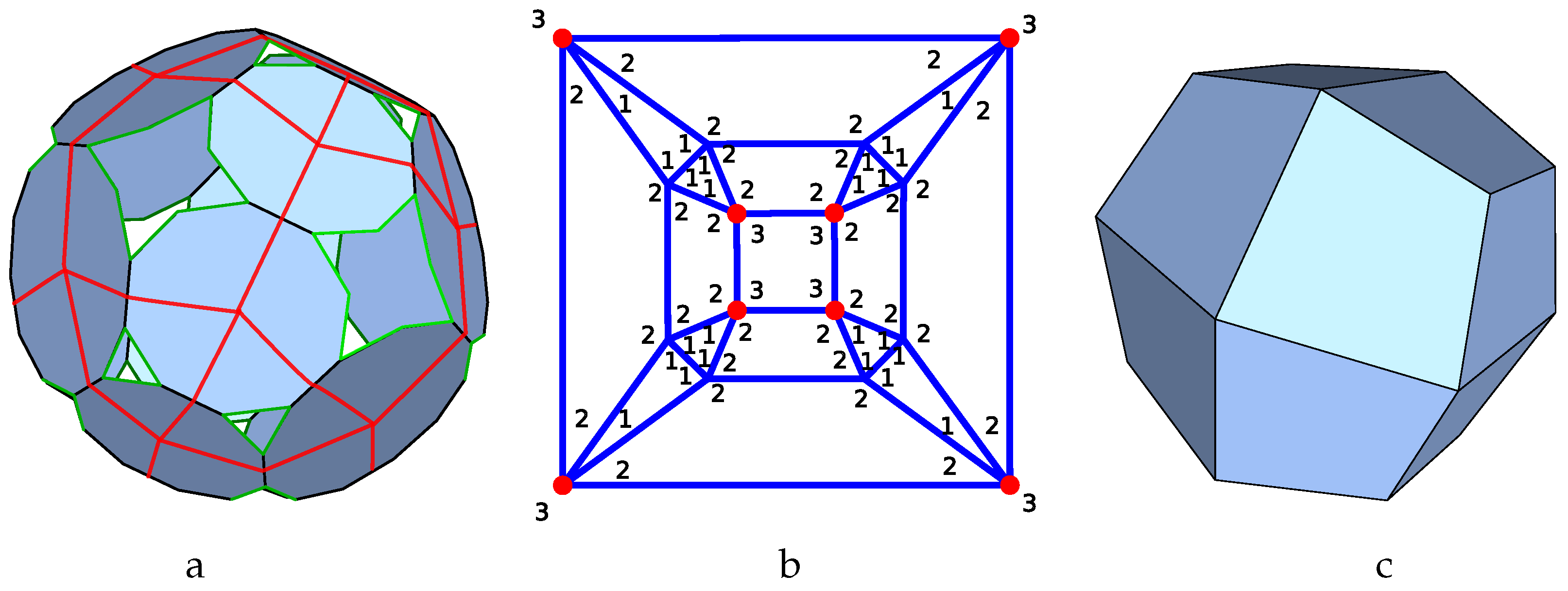
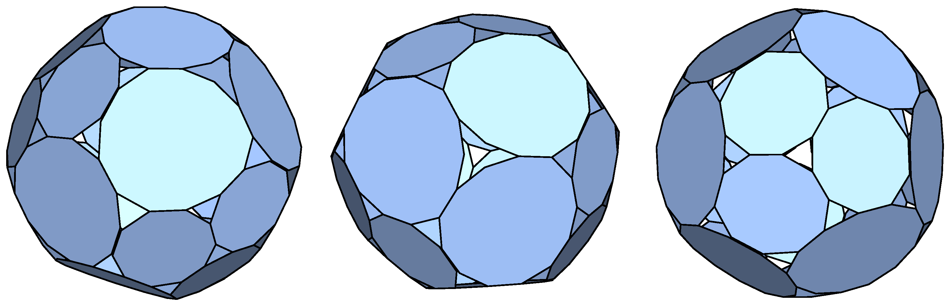
As outlined above, the connectivity between the faces of a p-cage is described by the so-called hole-polyhedron obtained by joining together the centre of the p-cage faces sharing edges. This is illustrated for a specific p-cage made out of decagons and dodecagons in
Figure 1a. The red lines define the edges of a polyhedron, which can be thought of as the dual of the p-cage.
Figure 1b corresponds to the planar graph of the hole-polyhedron. The nodes of the graph correspond to the p-cage faces, and the edges to the links between faces and the face of the graph describe the geometry of the holes. The number in each corner specifies the number of edges each face contributes to the adjacent hole. The dual solid of the hole-polyhedron,
Figure 1c, is the solid containing the p-cage, or phrased differently, one can obtain the p-cage by tilling the faces of the dual solid with the desired polygons. In what follows we refer to such solids as the tilling solid. The tilling solid is usually not unique as the faces can be deformed while preserving the planarity of the faces as well as their connectivity, and we will describe below how to identify the configurations leading to the least deformed tilling solids and p-cages.
The method we use to construct all the p-cages is outlined as follows: we start from one of the bi-equivalent planar graphs. Some of these graphs correspond to the planar graphs of regular solids or their dual solids, but most of them correspond to a regular solid to which one or more nodes have been added [
40]. The vertices of the regular solids can all be mapped into one another using the symmetry of that solid. The added vertices, when there are any, are also related to each other via the symmetries of the underlying solid. This means that we only need to consider a single face of each family, which we refer to as the reference faces, the other faces of the same families are obtained via a suitable rotation.
The faces of the p-cage will be polygons with
and
edges for, respectively, the face families I and II. By convention, following [
39,
43], we chose the family of type I to be the ones with the smaller number of neighbours.
Each reference face is described by the vertices
for
, ordered anticlockwise when seen from outside the p-cage, as well as
the normal to the reference face of type
j pointing towards the outside of the p-cage. The edges can then be described by the vectors
with the edge lengths given by
. The inside angles
between adjacent edges, are obtained by evaluating
and
Notice that if
is larger than
, the face is not convex. The angles between the adjacent edges of regular P-gons are all
. To minimise the deformations of the face, we evaluate all the
and
and minimise the regularity energy
where
with the 3 weight factors
,
and
. In (
3), the first term corresponds to the deviation of the edge lengths
from the target length
L while the second term measures the deviation of the inside angles,
, from that of a regular P-gon.
is given explicitly by
where
is the Heaviside function. Notice that (
4) is 0 unless the vertices describe a concave polygon.
To compute
we compute
, the centre of face
i and we consider 2 adjacent faces
and
with normal vectors
and
respectively. If, for all pairs of adjacent faces, the distance between the centres of the 2 faces is smaller than the distance between
and
, the p-cage is convex. This allows us to define
as
where
is the set of faces, of any type, adjacent to the reference face
j.
is non-zero 0 only for concave p-cages.
To minimise the irregularity of the p-cage faces as well as impose the convexity of both the p-cage and its faces, we use a simulated annealing algorithm [
44], which varies the parameters of the p-cages to minimise
E and hence determine the optimal configuration for each p-cage.
To enforce the convexity of the p-cage faces and of the p-cage itself, we take very large values for
and
, so that the last two terms in (
2),
and
dominate the energy contribution for concave faces and p-cage. Notice that in (
2) we divide the sum by
to make the parametrisation of the numerical optimising algorithm easier to tune.
To describe the regularity of the p-cages, it is useful to describe the amount of deformation as follows:
Each reference face is characterised by a vector normal to the face
, where
to label the two faces families, as well as 2 orthonormal basis vectors
and
so that any point on the plane span by the face can be described as
. The normal vector to the faces will be parameterised as follows:
Any face
k of the p-cage will span a plane described by the normal and orthogonal vectors
where
R is a rotation dictated by the symmetry of the underlying regular solid. For the reference faces
R is obviously the unit matrix.
To determine the edges of the p-cage faces, we have to parameterise the line intersecting the planes span by any two pairs of adjacent faces. Given two adjacent planes and their basis vectors
,
,
and
,
,
, we first define the normalised normal vectors,
and
, as well as the vector
parallel to the intersection of the 2 planes:
Next, we find the point
on the intersecting line
which is perpendicular to
by multiplying (
9) by
. This leads to a relation between
and
as well as
and
. Multiplying (
9) by
, we insert back into (
9) the obtained expression for
to obtain
Once we have the intersecting lines between 2 pairs of adjacent faces we will also need the intersecting point between these 2 lines:
Imposing the condition
and multiplying (
12) by
and also
leads to the equations
This system of two linear algebraic equations can easily be solved to find
When the hole polyhedron is a regular solid or the dual of a regular solid, the dual of the hole polyhedron, the tilling solid, is known and can be tilled with the required polygons as described later.
When the hole polyhedron planar graph is that of a regular solid to which one or more nodes have been added, the two families of faces correspond to the face related to the vertices or the regular solid, which we call the solid faces, and those corresponding to the added vertices, which we call the extra faces.
To construct the tilling solid, i.e., the dual of the hole polyhedron, we take one of the regular solid vertex as the normal to the reference solid face. The normal to the extra faces is taken somewhere on the face to which it has been added. All the other faces of the tilling solid are related to each other via the symmetry of the underlying regular solid. We then consider the intersection lines between the reference faces and each of their adjacent faces using (
7) and (
10). Going round the reference face, we then compute the intersecting points (
11) between the consecutive intersecting lines to obtain the vertices of the tilling solid. As the solid is usually not unique, we can optimise it so that the length of the face edges are as similar as possible, and this can be performed by optimising (
2) where, in this case, all the vertices are shared between at least 3 faces (no holes).
Once we have the tilling solid, we use the normal of its reference face as the initial normal vector for the p-cage reference faces. One might wonder why the two steps are necessary rather than optimising the p-cage directly. The reason is that finding good initial normal vectors for the p-cage faces is quite tricky for some of the more irregular tilling solids, and optimising the tilling solid must only be performed once. Then one can more easily optimise all the p-cages of that class (same graph), which sometimes includes several tens of thousands of different configurations, starting from the tilling solid.
From each hole polyhedron graph, we can generate a number of p-cages by choosing different polygons for the p-cage faces. Moreover, if a P-gon face shares n edges with as many neighbours, there are edges to distribute between the holes. This must be performed in such a way as to preserve the equivalence between the faces of each family, and we do this by labelling the corners of the hole-polyhedron graph with the symbols a,b,c,d,e and A,D,C,D,E,F for respectively the type I and II families. Once we have placed the first label, a or A we place the others anticlockwise around each vertex in alphabetical order. In a few cases it is more convenient to label the planar graph of the tilling solids, in which case the labels are placed anticlockwise around each face.
To minimise (
2) we have used an annealing algorithm. In units of the energy (
2), the temperature was decreased from
to
by the multiplicative factor
with 2000 randomisation per degree of freedom for each temperature. The parameters
and
were both set to 10,000.
and
where initially both set to 1 and then varied using the steepest descent algorithm, minimising the function
, while maintaining the constraint
. A full simulated annealing relaxation was performed for each value of
and
.
Before describing the derivation of the p-cages configurations, we must describe the naming scheme that we use to label them: the p-cages are named after the graphs they are built from, the size of the face and the number of edges contributing to the holes as follows: GRAPH_P_P_a_b_c_d[_e]-A_B_C_D[_E_F] where the italic symbols are replaced by actual values. To avoid very long names, we also use a simplification when n successive hole-edge labels have the same values, , by replacing the sequence by nx. So, for example, p5-2pyr_P10_P10_2x1_2x2-5x1 is equivalent to p5-2pyr_P10_P10_1_1_2_2-1_1_1_1_1.
We will now describe six typical examples, the others being described in the
Supplementary Materials. In the first example, the tilling solid is a regular solid, so one just needs to tile it to obtain p-cages. In the second example the hole-polyhedron graph is an antiprism, and we use a simple geometric construction to construct the tilling solid. The same method was used to construct the tilling solid of the axially symmetric graph, which does not correspond to any regular solid. In the third example the hole-polyhedron graph corresponds to the planar graph of a regular solid to which one node has been added to some of the faces. In the forth example the hole-polyhedron graph corresponds to the planar graph of a regular solid to which three nodes have been added to some of the faces. The last 2 examples cover cases where the faces have more neighbours.
The graphs that we have considered are all listed in
Appendix A together with the planar graph name from [
40], the p-cage name, the number of configurations that we have tested as well as the number of p-cage found with deformations not exceeding 10% and 5%.
3. Some Examples
In what follows we will detail the six examples outlined above. The other classes of bi-symmetric p-cages are detailed in the
supplementary files.
2-4pyr:
The first case we consider is the planar graph named
44_F8_8-2-1_V4_2 in [
40]. It corresponds to the solid consisting of two back-to-back square-base pyramids. Its dual solid is a square prism, and the faces belonging to the first family are placed on the sides of the prism, while the two faces belonging to the second family are placed at the top and the bottom face of the prism.
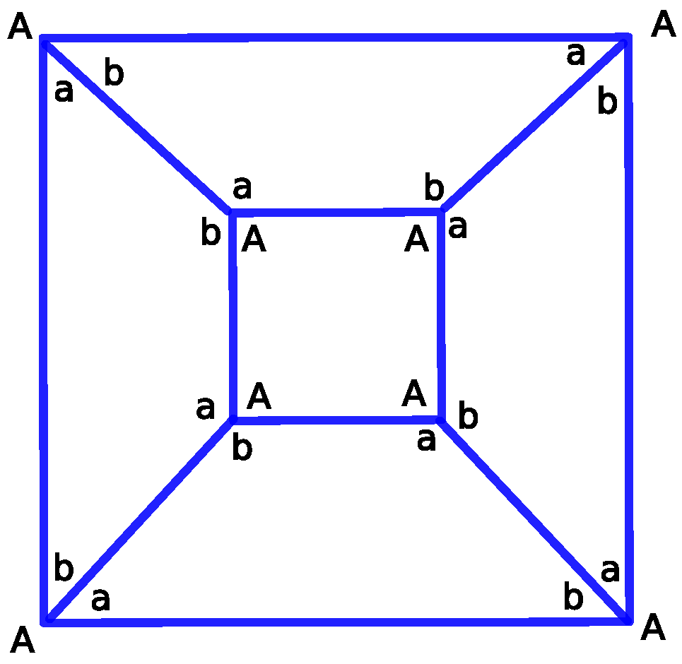
The hole-edge contribution of each face is very much constrained by the axial symmetry of the p-cage.
Figure 2 displays the possible numbers of edges that each face can contribute to the holes while preserving the equivalence between each family of faces. The graph corresponds to the planar graph of the tilling solid. While the faces of the second family must contribute the same number of edges, marked
A in
Figure 2, to each of the holes to which they are adjacent, the faces of the first family must contribute the same number of edges, marked as
a and
b in
Figure 2, to the holes that are diagonally opposite to each others. If we swap
a and
b, we obtain a p-cage equivalent modulo a reflection, and this allows us to consider fewer configurations. As we restrict ourselves to no more than three edges per hole, we must only consider the following hole-edge configurations for the first family of faces:
[1,1,1,1],
[2,2,2,2],
[3,3,3,3],
[1,2,1,2],
[1,3,1,3] and
[2,3,2,3] for
[a,b,c,d] while for the second family of faces we only consider
[1,1,1,1],
[2,2,2,2]and
[3,3,3,3] for
[A,B,C,D], for a total of 18 configurations.
The vectors and are chosen to point respectively to the centre of a side face () and the top face () of the square prism.
The result of minimising (
2) is that the only p-cages with deformations below 10% are the ones with
, all of which are regular (see the
supplementary files). When
, this corresponds to the truncated cube where the triangles are the holes of the p-cage.
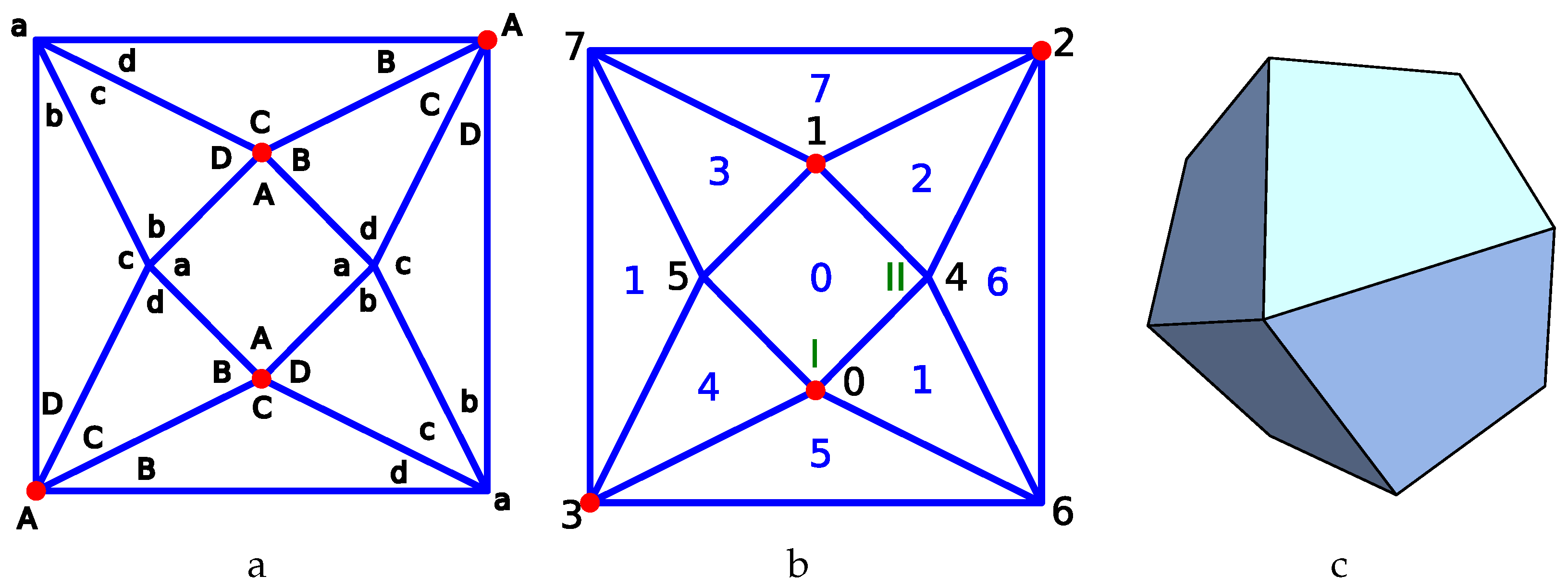
a4-alt:
Next we consider the planar graph named
44_F10_2-2-2_4-1-2_4-2-1_V4_4 in [
40]. It corresponds to a square base antiprism where the two types of nodes alternate between the bases as shown in
Figure 3a. If we swap simultaneously
b with
d as well as
B with
D, we obtain the same p-cage after a reflection, so that if we consider all values from 1 to 3 for the hole-edge parameters, we obtain
3645 different configurations to test.
Figure 3b describes the parametrisation used to build the tilling solid. It can be visualised as the planar graph of a square antiprism. The vertices
and
belong respectively to the second and first family of faces. The angles for the vectors
and
are
,
, (vertex
I on the figure) and
,
, (vertex
II on the figure). Moreover the references faces have index 4 and 0 and reference faces and the other faces are related as follows:
where
corresponds to a rotation of and angle
around the
axis. One can then use (
10) to derive numerically the coordinates of the line of intersection between the adjacent faces, and then the intersection between these lines determines the vertices of the tilling solid as shown in
Figure 3c. As in the previous case, the normal vectors can also be adjusted numerically to obtain a tilling solid which is as regular as possible.
The normal vectors to the faces of the tilling solid are then used as the initial normal vectors to the reference faces of the p-cages, and one minimises (
2) numerically to obtain the most regular p-cages.
In this example we only obtained 16 and 4 p-cages with deformations not exceeding 10% and 5% respectively. The ones with less than 5% deformation correspond to the parameters [1,3,3,3;2,3,3,3] (), [3,2,2,2;3,2,2,2] ( ), [2,1,1,1;3,1,1,1] () and [3,1,1,1;2,1,1,1] (), where the brackets correspond to the values [a,b,c,d;A,B,C,D].
The first one of these is shown in
Figure 4.
p5-2pyr:
The third case we consider is the planar graph named
45_F15_5-4-0_10-2-1_V10_2 in [
40]. It corresponds to a pyramid added on top of the bases of a pentagonal pyramid. as illustrated in
Figure 5a.
If we swap simultaneously a with b as well as c with d we obtain the same p-cage after a reflection and as a result, if we consider all values from 1 to 3 for the hole-edges parameters there are 135 different configurations to test.
Figure 5b describes the parametrisation used to build the tilling solid.
is chosen as vertex 0 of the prism while
is chosen as the centre of face 0. Vertices 1–9 of the solid are related via the symmetries of the pyramid, and they translate into the symmetry between the p-cage faces belonging to the first family. The two faces of the second family are related via the same symmetry as the one transforming face 0 and 6 of the prism.
One of our computer programs was used to compute the tilling solid corresponding to that graph and to optimise it so as to make the edge lengths as identical as possible. The result is displayed in
Figure 5c.
To optimise the p-cage, the normal vectors and were chosen initially as the normal vectors to the reference face of the tilling solid.
This lead to 12 p-cages with deformations below 10% and 7 p-cages with deformation below 5%: [1,1,3;1,1,1,1]() which is a degenerate case corresponding to the truncated tetrahedron where the triangles are the holes, [1,1,2,2;1,1,1,1] () which corresponds to a regular p-cage within our numerical accuracy, [2,2,3,3;2,2,2,2] (), [1,1,2,3;1,1,1,1] (), [3,3,3,3;3,3,3,3] (), [2,2,2,2;2,2,2,2] () and [1,1,1,1;1,1,1,1] ().
The second one of these is shown in
Figure 6.
Att-hex-4star:
The next family of p-cages that we consider in detail corresponds to the planar graph named
45_F32_4-0-3_4-3-0_12-1-3_12-2-1_V12_12 in [
40]. It corresponds to a truncated tetrahedron on which what is called a polygonal star in [
40] is added to each hexagon. This is illustrated in
Figure 7b, where the polygonal stars are drawn in red.
Figure 7a illustrates a partial labelling of the edge-hole contribution of each face. A figure showing the full graph is available in the
Supplementary Materials. If we swap simultaneously
b with
d,
B with
E as well as
C with
D, we obtain the same p-cage after a reflection, so that to consider all values from 1 to 3 for the hole-edges parameters we must test
10,206 different configurations.
Figure 7b describes the parametrisation used to build the tilling solid. For the optimisation,
is initially chosen as vertex 0 of the truncated tetrahedron while
is initially chosen as the point halfway between vertex 0 and the centre of face 4. The 12 vertices of the truncated tetrahedron are related to the 12 faces of type 2 of the p-cage and are mapped into one another via the symmetry of the truncated tetrahedron.
The reference face of type I is mapped onto the other two faces of the same type added on face 4 of the truncated tetrahedron via a
rotation around the centre of that face. The other faces of type I are mapped from these three faces via the symmetry mapping of the hexagonal faces of the truncated tetrahedron. The resulting tilling solid is presented in
Figure 7c. This is an example where the tilling solid is not easy to obtain due to its somewhat irregular and twisted nature. Once it was obtained, the normal of its reference faces were used as initial normal vectors for the p-cage faces to generate the
10,206 different p-cages.
This resulted in only five p-cages with deformation below 10% and none with deformation below 5%. The least deformed p-cage is shown in
Figure 8.
p4-split6-sqr:
The next family of p-cages that we consider in detail corresponds to the planar graph named
46_F26_2-0-4_8-2-1_1-16-1-2_V8_8 in [
40]. It corresponds to a 4-prism where the side squares are split into six triangles as illustrated in
Figure 9b where the triangles are drawn in red.
Figure 9a illustrates a labelling of the edge-hole contribution of each face. This graph does not have any symmetries, so considering all values from 1 to 3 for the hole-edge parameters, we must test
= 59,049 different configurations.
Figure 9b describes the parametrisation used to build the tilling solid.
is initially chosen as vertex 0 of the truncated tetrahedron while
is initially chosen as the point halfway between vertex 0, vertex 4 and the centre of face 1. The eight vertices of the 4-prism are related to the eight faces of type I of the p-cage via the symmetry of the 4-prism. The added vertices, shown in red in
Figure 9b, are related to the eight faces of type II. The two vertices of type II on a given face are related to each other via a
rotation around the centre of that face. The vertices on the other faces are obtained via the symmetries of the 4-prism.
The resulting tilling solid is presented in
Figure 9c. Once it was obtained, the normal of its reference faces was used as initial normal vectors for the p-cage faces to generate all the different p-cages. This resulted in only one p-cage with deformation below 10%, which is shown in
Figure 10.
Arcd-pen-pyr:
The final family of p-cages that we consider corresponds to the planar graph named
55_F110_20-3-0_30-4-0_60-2-1_60_12 in [
40]. It corresponds to a pentagonal pyramid placed on the pentagons of the rhombicosidodecahedron. This is illustrated in
Figure 9b, where the pyramids are drawn in red.
Figure 11a illustrates a labelling of the edge-hole contribution of each face on part of the tilting solid. If we swap simultaneously
a with
b, as well as
c with
d, we obtain the same p-cage after a reflection. As a result, to consider all values from 1 to 3 for the hole-edge parameters, we must test
405 different configurations.
Figure 11b describe the parametrisation used to build the tilling solid.
is initially chosen as a vertex of the rhombicosidodecahedron while
is initially chosen as the centre of the adjacent pentagonal face. The vertices of a given type are all related to each other via the symmetry of the rhombicosidodecahedron.
The resulting tilling solid is presented in
Figure 11c. Once it was obtained, the normal of its reference faces was used as an initial normal vector for the p-cage faces to generate all the different p-cages. This resulted in only 39 p-cages with deformation below 10%. The least irregular one is shown in
Figure 12.
4. Results
We have identified a large number of bi-symmetric p-cages with small holes and with faces joined with at least four neighbour faces. We have considered 58 hole polyhedron planar graphs leading to over 600,000 p-cage configurations to optimise, but only a small number of them have deformations not exceeding 10%. The detailed derivations of all the p-cage families considered are provided in the
Supplementary Materials.
Some of the p-cages correspond to the tilling of the faces of regular solids, with either one p-cage face per face of the solid or P p-cage face for a P-gon solid face. For these last cases, the dihedral angles between adjacent faces take very different values, making these p-cages look like poor choices for protein nanocages.
Some of the p-cages we have found after numerical optimisation are degenerate in the sense that two edges that are not meant to be merged do so, increasing the number of neighbours per face and hence being identical to a p-cage of the different category. This is the case, for example, with the p-cage
Att-3fan_P11_P11_2x1_2_3-2x1_2_3, which is identical to the symmetric p-cage
Asc_P11_2_1_1_1_1 described in [
36,
37]. For completeness, it makes mathematical sense to include these degenerate geometries in our list. Moreover, should a laboratory be able to add linkers selectively [
45] only to the face edges which the geometry dictates to merge with neighbour faces, the resulting degenerate p-cage would have the same geometry as the non-degenerate one except that some edges would be adjacent, i.e., touching, without being actually linked together.
Some of the p-cages we have obtained as the result of the numerical optimisation are also identical to symmetric p-cage because their faces can be split into two different families. This is the case, for example, for the p-cage
Att-3fan_P11_P11_1_3x2-1_3x2, which is identical to the symmetric p-cage
Arco_P11_1_2_2_2 [
36,
37].
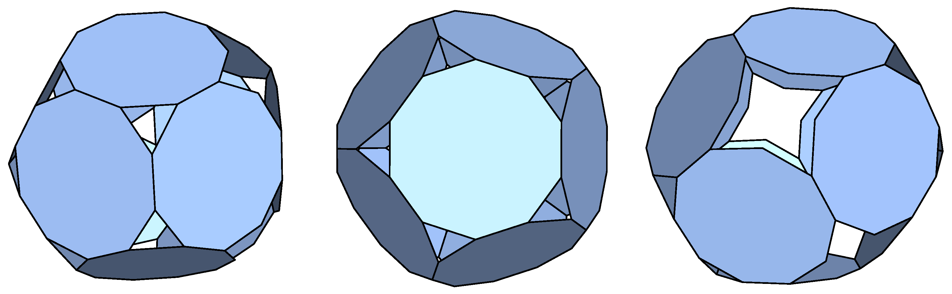
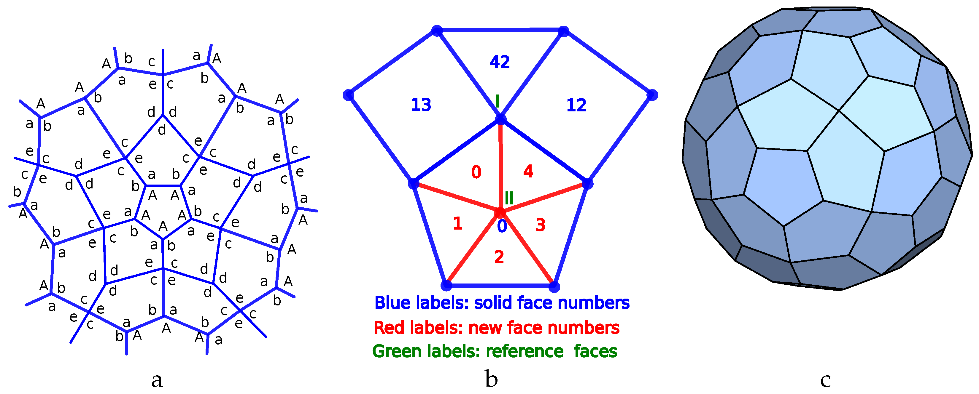
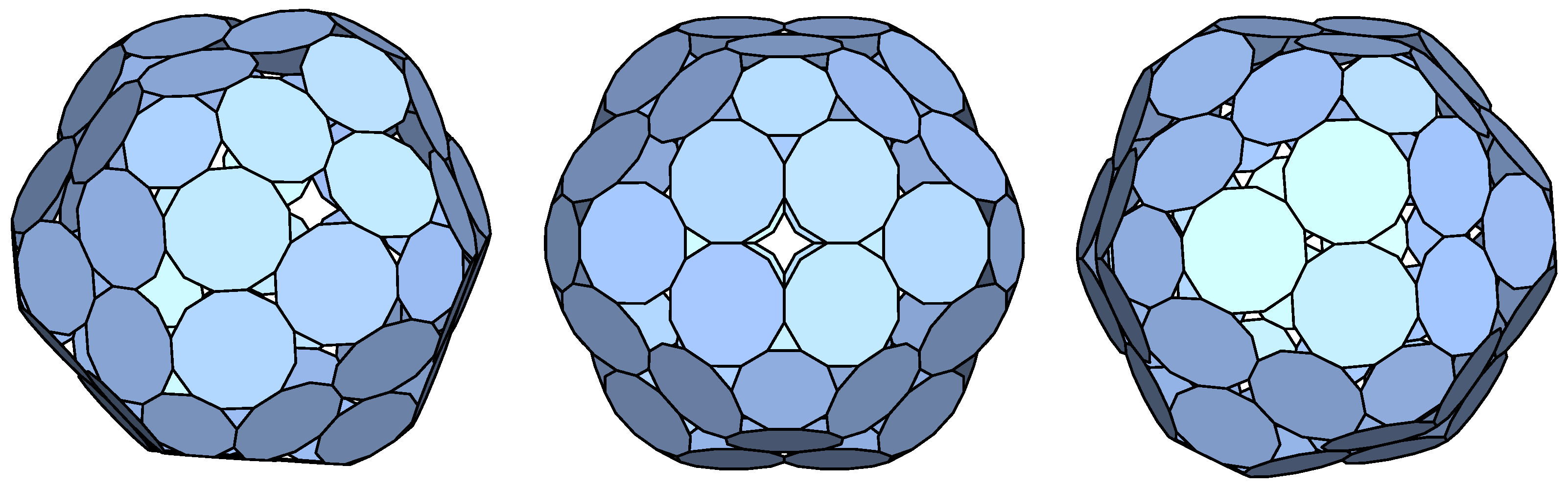
We now describe a few p-cages that correspond to good geometries for protein nanocages due to their near regularity. We include three viewing angles of each p-cage as well as either their hole-polyhedron graph or the planar graph of the tilling solid. The red dots on the hole-polyhedron graphs correspond to the p-cage faces of family II. In each case we provide the relative deformations and as well as and , which are, respectively, the number of faces of types I and II.
In
Figure 13 and
Figure 14 we present two p-cages based on the same planar graph corresponding to what is called in [
40] two inverted fans back to back. Both families of faces have four neighbours each. The first one is made out of 12 decagons and the second of 12 hendecagons. In both cases the polygons are split into two different families.
The p-cage shown in
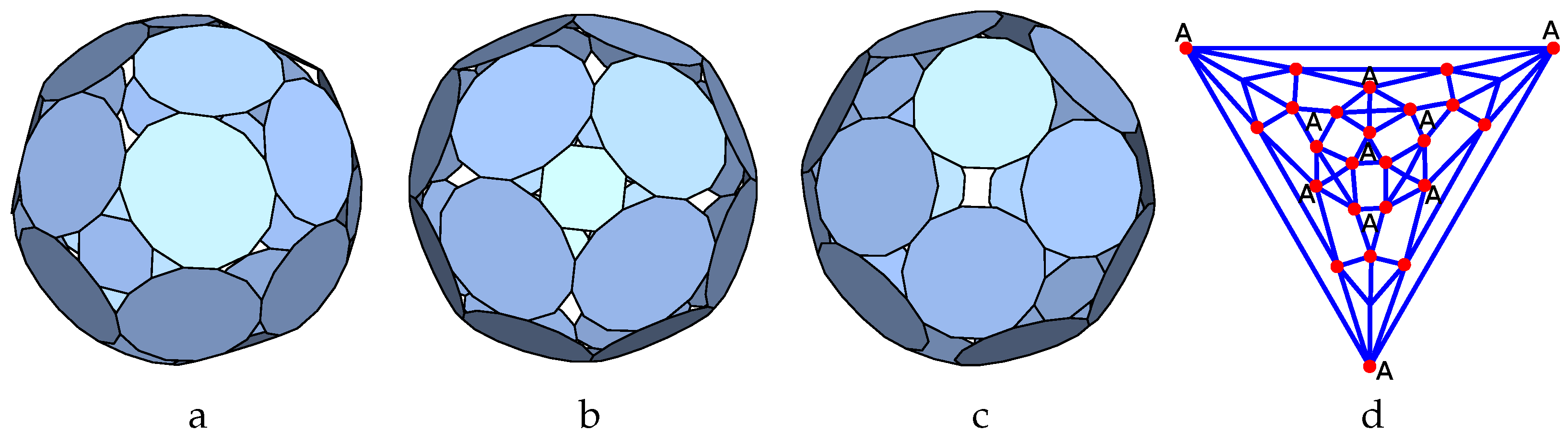
Figure 15 is made out of 24 decagons and 6 octagons. The four hole-edge contributions of the type II faces, the octagons, must all be identical, while the four hole-edge contributions of the type II faces are arbitrary. The labels
a are placed on the triangles formed by three type I nodes (the ones with no red dots).
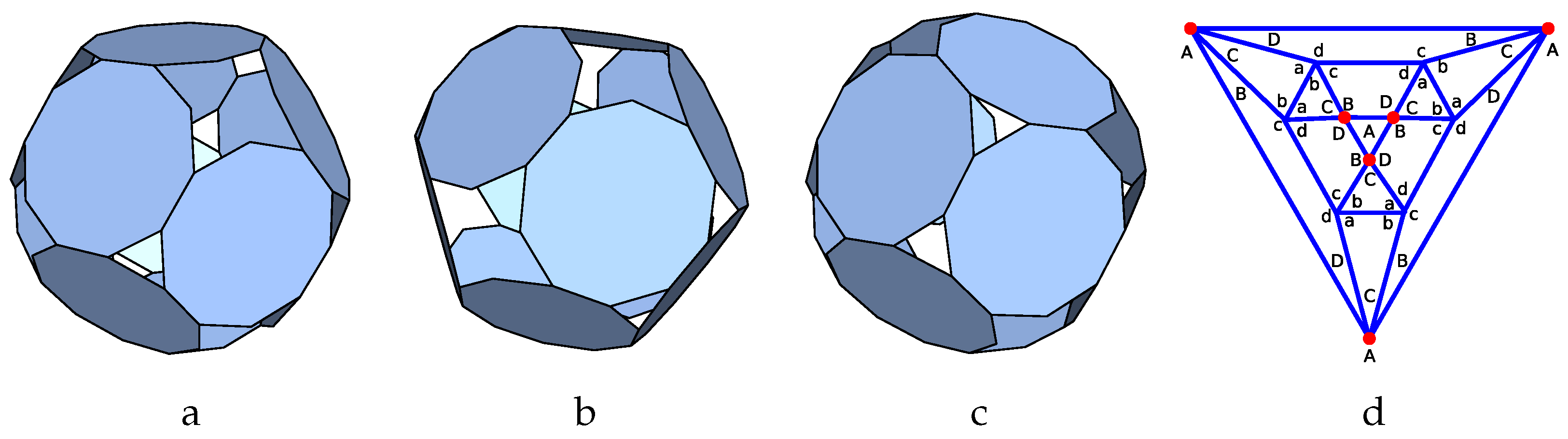
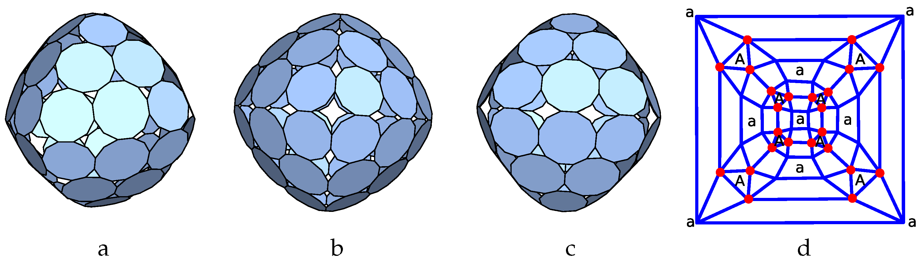
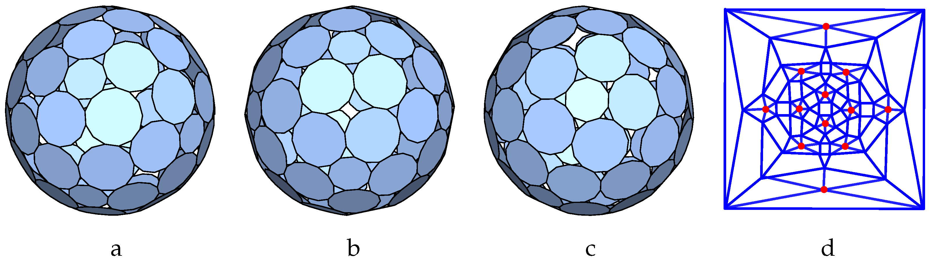
Figure 16 describes the p-cage
Att-3fan_P10_P10_2x1_2x2-2x1_2x2 made out of 24 decagons. The planar graph of the tilling solid is shown in
Figure 16d; each face of the graph corresponds to a face of the p-cage.
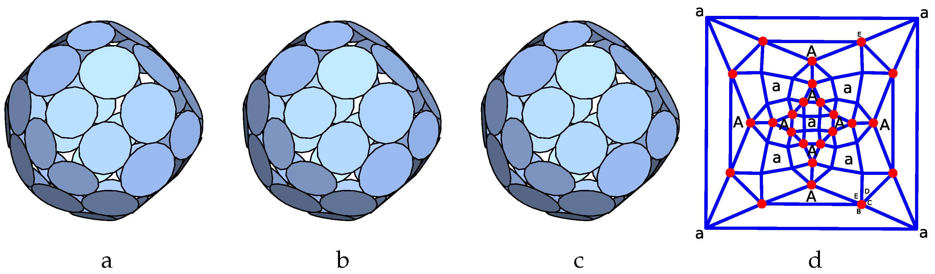
In
Figure 17 we present the p-cage
Arco-6sqr-pyr_P8_P14_4x1-2x2_2x1_3 made out of 6 octagons and 24 14-gons. The four hole-edge contributions of the type I faces, the octagons, must all be identical, while the hole-edge contributions of the type II faces are arbitrary. The label
A is placed onto the triangle formed by three type II nodes.
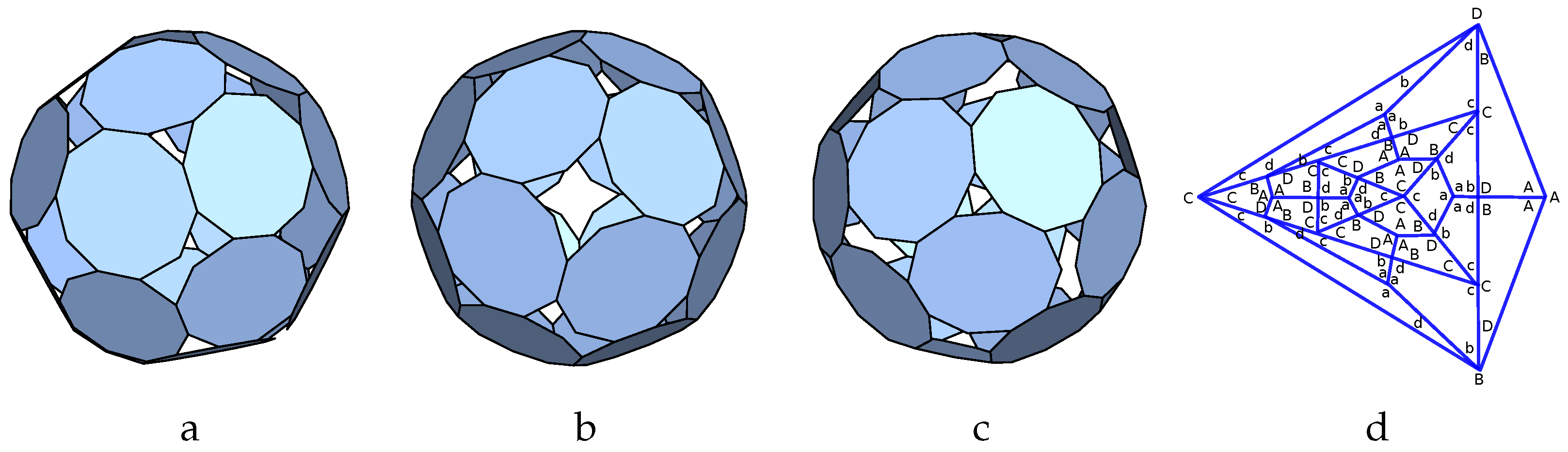
Figure 18 describes the p-cage
Atc-oct-6fan_P11_P12_2x2_1_2-2x1_2x2_1 which is made out of 24 hendecagons and 24 dodecagons. The four hole-edge contributions of type I faces and the five hole-edge contributions of type II faces can take any value. The labels
a are placed on the squares formed by four type I nodes, while the labels
A are placed in the triangles formed by three type II nodes.
The p-cage
Atc-oct-6fanb_P15_P18_2x3_2_3-2x3_2x2_3 is shown in
Figure 19. It is made out of 24 15-gons and 24 18-gons. The 15-gons have four neighbours while the 18-gons have five. The four hole-edge contributions of type I faces and five hole-edge contributions of type II face can take any value. The labels
a are placed on the squares formed by four type I nodes, while the labels
A are placed in the triangles formed by three type II nodes.
Figure 20 shows the p-cage
Pt-invfan_P10_P12_2x1_3_1-6x1. It is made out of 12 15-gons and 4 18-gons. The 15-gons have four neighbours, while the 18-gons have five. The four hole-edge contributions of the type I faces can take any value, while the five hole-edge contributions must take alternating values
A and
B for the type II faces. The labels
a are placed on the triangles formed by three type I nodes, while the labels
A are placed on the squares adjacent to the type II nodes, while the labels
B are placed on the adjacent triangles.
Figure 21 shows the p-cage
Pc-invfan_P11_P12_2_1_3_1-6x1, which is made out of 24 hendecagons and 8 dodecagons. The hendecagons have four neighbours while the dodecagons have five. The four hole-edge contributions of the type I faces can take any value, while the five hole-edge contributions must take alternating values
A and
B for the type II faces. The labels
a are placed on the squares formed by four type I nodes, while the labels
A are placed on the squares adjacent to the type II nodes and the labels
B are placed on the adjacent triangles.
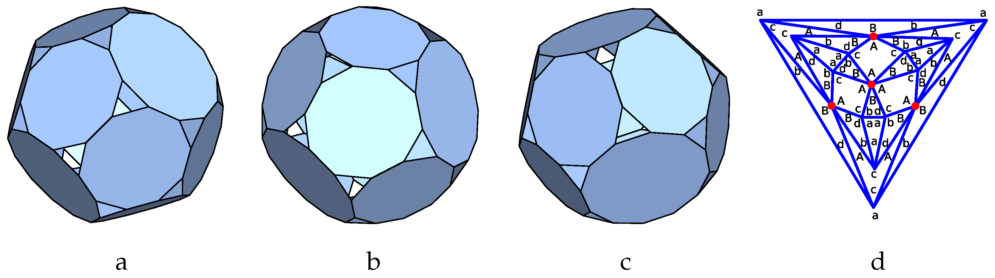
In
Figure 22 the p-cage
Arcd-pen-pyr_P13_P10_2x1_2_1_3-5x1 is shown as made out of 60 13-gons and 12 decagons. Both types of faces have five neighbours. The hole-polyhedron graph corresponds to a rhombicosidodecahedron on which a 5-pyramid is placed on each pentagonal face. The five hole-edge contributions of the type II faces must take the same value
A, while the five hole-edge of type I face can take any value. The labels
a are placed anti-clockwise next to the labels
A.
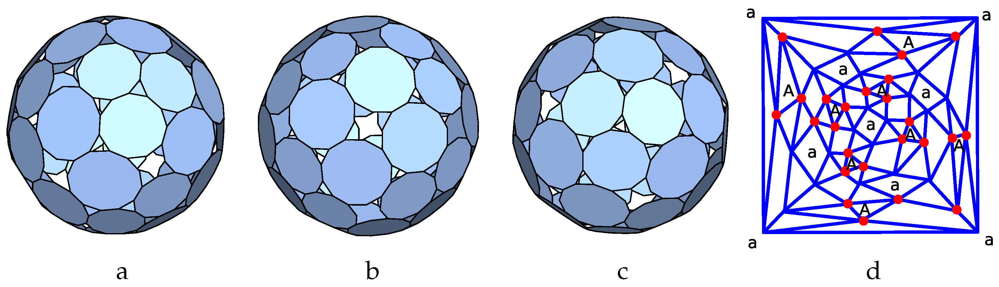
Finally, the p-cage named
Ato-hex-sfan_P12_P11_2_2x1_2_1-3x1_2_1 is presented in
Figure 23. It is made out of 24 dodecagons and 24 hendecagons. The hole-polyhedron graph corresponds to a truncated octahedron on which a split fan is placed on each hexagon. The five hole-edge contributions of the type I and II faces can take any value. The labels
a are placed on the squares made by four type I nodes, while the labels
A are placed on the triangles made by three type I nodes.


