Identifying Vital Nodes by Local g-Core on Symmetric Networks

Abstract

The H-index is a widely recognized centrality measure for nodes in symmetric networks, defined as the maximum number of neighbors with degrees equal to or greater than the node’s own degree. However, this metric underestimates the structural influence of “weak nodes”—low-degree nodes connected to high-degree hubs—that often serve as critical connectors in network topology. To address this limitation, we propose the $H_{\alpha }$-index, which generalizes the H-index by considering the maximum number of neighbors with degrees at least $\alpha$ times the node’s degree, where $\alpha \ge 1$. Based on this refinement, we introduce two novel centrality measures: the g-core and the local g-core, which were derived from iterative applications of the $H_{\alpha }$-index to a node’s neighbors. Extensive experiments on sixteen real-world networks demonstrate the efficiency of our methods. Notably, the local g-core achieves 45–105% higher Kendall Tau correlation coefficients compared to the traditional H-index and coreness on three benchmark networks, highlighting its superior performance in capturing node influence.

1. Introduction

Identifying influential nodes [1,2,3,4,5,6] in complex networks [7,8,9] remains a persistent challenge, with critical applications spanning targeted advertising on social platforms, source localization in rumor propagation, and the selection of high-impact researchers.

In the context of various methods for assessing scientific influence, one prominent metric is the H-index [10], which has emerged as a widely adopted metric to quantify both the quality and productivity of the research output. Originally proposed by J. E. Hirsch to characterize individual scientific contributions, the H-index has since been extended to evaluate academic institutions and journals [11]. By integrating measures of publication quality (impact factor) and quantity (publication count), it addresses the limitations of traditional metrics that prioritize only one dimension.

Over the past two decades, the H-index has attracted significant attention from scientometrics researchers proposing various improvements in different perspectives [12,13,14,15,16,17,18,19,20,21,22,23,24,25,26,27]. These advancements fall into three primary categories: (I) Normalization and Averaging: Methods such as normalizing the H-index by the number of authors [14], by the publication year [15], and by the disciplinary field [16], as well as by averaging with citation counts [17] or geometric mean [18]. (II) Incorporation of Additional Information: Approaches that integrate auxiliary data, including the author’s position in bylines [19], the shape of citing functions [20], subdomain distributions within a scientist’s citation profile [21], the collaboration distance between citing and cited authors [22], excess citations beyond $H^2$ citations for papers [23], and the inclusion of uncited papers [24]. (III) Temporal Evolution Analysis: Studies examining the H-index’s trajectory over a researcher’s career, such as predictive models via regression analysis [25,26] and time window evaluations [27].

These improvements, though valuable, are closely tied to the intrinsic properties of papers and authors, making generalization to broader complex networks challenging.

Notably, the H-index has also captured the interest of scholars in complex networks since Lü et al. [28] revealed the H-index’s relationship to degree and coreness. Specifically, Lü et al. [28] defined an H-operator on a group of numbers via the H-index. They proved that the coreness—a centrality measure introduced by Kitsak et al.—is the limit of the iteration of the H-operator. This seminal work [28] has sparked widespread attention. On the one hand, it has been extended to directed networks [29] and weighted networks [30]. On the other hand, it has reinvigorated interest in coreness, a computationally efficient centrality metric. Despite its utility, coreness has inherent limitations, such as limited discrimination power and coarse-grained resolution, which can hinder its application in certain contexts. To address these, several refinements have been proposed, including mixed degree [31], shortest distance-based coreness [32], community-based coreness [33], coreness without redundant links [34], and two-step coreness [35].

This paper investigates the limitations of the H-index in capturing the influence of weak nodes—nodes with small degrees but high-degree neighbors. Our analysis is driven by the observation that the H-index, which counts neighbors’ degrees, underestimates the influence of weak nodes. For example, consider two nodes: Node u has neighbors with degrees $\{3,3,3\}$, yielding $H\left(u\right)=3$ and highlighting that it is indeed a weak node. Node v has neighbors with degrees $\{10,10,10\}$, also yielding $H\left(v\right)=3$. Although node v is a weak node (low degree but surrounded by high-degree neighbors), it is more influential in information propagation than node v. This illustrates a critical shortcoming of the H-index: specifically, it assigns equal influence to nodes with structurally distinct neighbor sets.

The k-core decomposition, derived by iteratively applying the H-index to a node’s neighbors, exacerbates this bias. Weak nodes are systematically underestimated in k-core analyses due to their low intrinsic degrees, despite their high-degree neighbors.

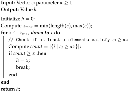
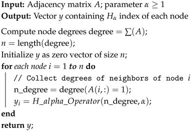
To estimate the influence of weak nodes during information spreading, we propose a new centrality, the $H_{\alpha }$-index, which is the maximum number of neighbors with at least $\alpha$ times the node’s degree. This formulation emphasizes relative neighbor quality (via $\alpha$) over absolute degree thresholds, enabling nuanced influence quantification.

Building on the $H_{\alpha }$-index, we define the g-core, a hierarchical decomposition that partitions the network based on $H_{\alpha }$-index values. This method better captures the influence of weak nodes compared to the traditional k-core.

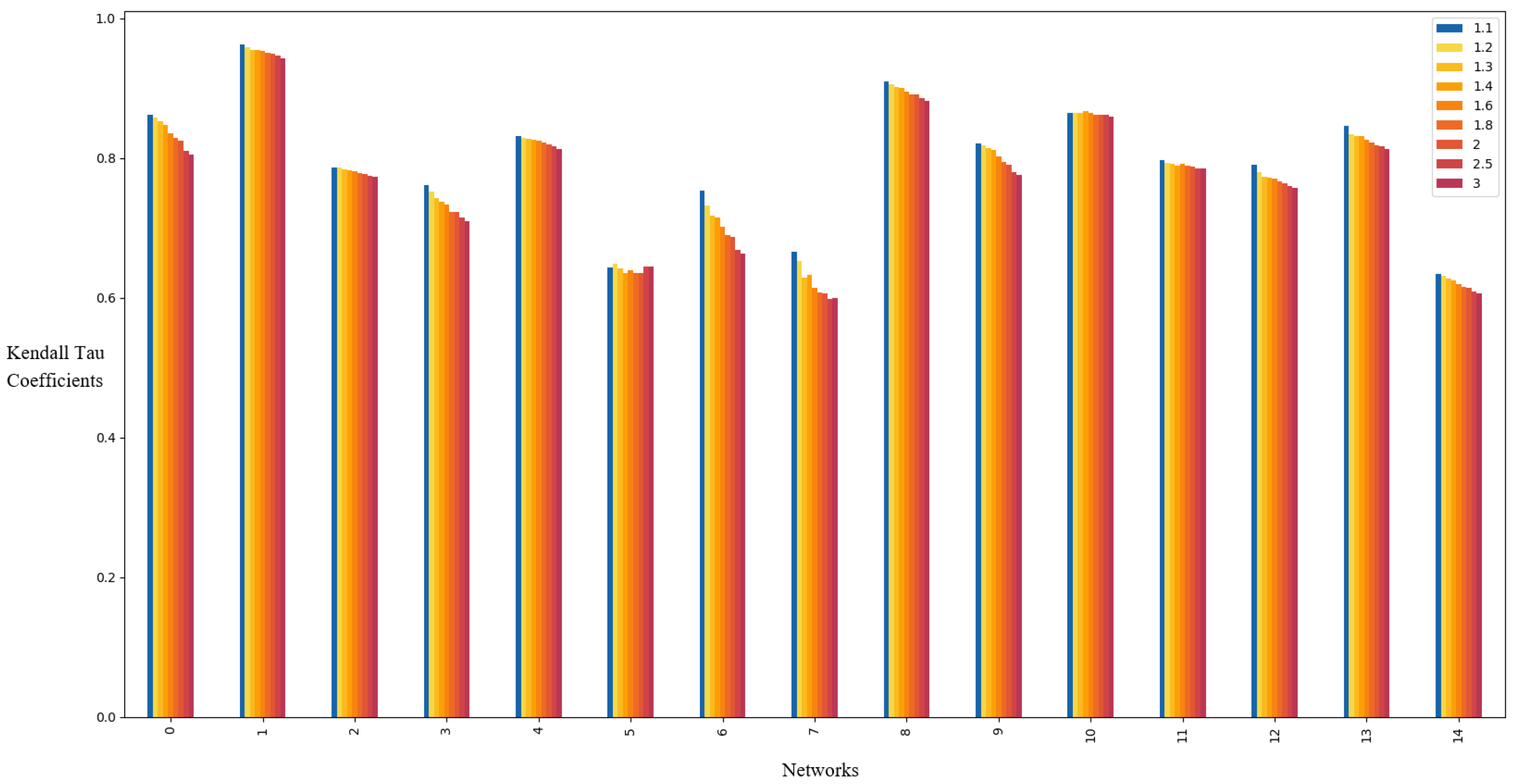
The rest of the paper is organized as follows: Section 2 provides the theoretical background on the H-index, k-core, and collective influence centrality. Section 3 introduces the $H_{\alpha }$-index, the g-core, and the local g-core. Section 4 presents experiments validating the superiority of the $H_{\alpha }$-index and g-core. Section 5 discusses future research directions.

2. Classical Centrality

2.1. Notations

Let $G(V,E)$ denote an undirected symmetric network, where V and E represent the set of nodes and the set of edges in G, respectively. The adjacency matrix $A={\left(a_{uv}\right)}_{n\times n}$ encodes connectivity, where $n=\left|V\right|$ is the number of nodes in G and $a_{uv}=1$ if nodes u and v are connected, i.e., $(u,v)\in E$, and $a_{uv}=0$ otherwise. The neighborhood $N_G\left(v\right)$ of the node v is defined as the set of nodes directly connected to v. For a node v, let $k_v$ denote its degree, i.e., $|N_G\left(v\right)|$.

2.2. H-Index Centrality

Definition 1. 

Let $\Omega =\{x_1,x_2,\dots ,x_m\}$ be a finite non-empty set of positive real numbers. Define the subset $T_y\subseteq \Omega$ as   

$$T_y=\{x_j\in \Omega \mid x_j\ge y\}.$$

The H-operator, denoted as $H(\Omega )$, is the maximum value y such that $|T_y|=y$.

Definition 2. 

Let v be a node in the graph G, and let $N_G\left(v\right)$ denote its neighborhood. The H-index of v, denoted as $h_v$, is defined as

$$h_v=H\left(\{k_u\mid u\in N_G\left(v\right)\}\right),$$

where $k_u$ is the degree of node u.

2.3. Coreness Centrality

Coreness centrality is a network topological measure derived from k-core decomposition. It evaluates a node’s importance based on its position within the hierarchical core structure of a network. Nodes with higher coreness values occupy denser, more central regions of the network, playing critical roles in maintaining global connectivity and influence.

The k-core is obtained through iterative degree-based pruning:

(1).

Start with the original graph $G=(V,E)$.

(2).

Iteratively remove all nodes with a degree less than k along with their incident edges.

(3).

Repeat until no nodes with a degree less than k remain.

The resulting subgraph is the k-core. The node v is assigned a coreness of $c_v=k$ if it belongs to the k-core but not the $(k+1)$-core. This hierarchical decomposition ensures that nodes in higher k-cores are more deeply embedded within the network’s core structure.

2.4. Closeness Centrality

Closeness centrality measures a node’s centrality based on its average distance to all other nodes in the network. It quantifies how quickly a node can reach others, reflecting its efficiency in spreading information or influence. Nodes with high closeness centrality are “close” to others, meaning that they have short average path lengths to all nodes.

The closeness centrality $cc\left(v\right)$ of the node v in the connected graph $G=(V,E)$ with n nodes is defined as

$$cc\left(v\right)={\displaystyle \frac{n-1}{{\sum }_{u\ne v}d(u,v)}},$$

where $d(u,v)$ is the shortest path length between nodes u and v and $n-1$ normalizes the measure to account for the number of other nodes in the network.

2.5. Collective Influence Centrality

Collective influence (CI) is a method developed by Morone and Makse [36] for identifying highly influential nodes in complex networks. CI quantifies a node’s influence by measuring the extent of damage inflicted on the network’s giant connected component upon the node’s removal. The formal definition of CI is given by

$$ci\left(u\right)=(k_u-1)\sum _{v\in \partial D(u,l)}(k_v-1),$$

where $k_u$ represents the degree of node i, $\partial D(i,l)$ denotes the set of nodes at a l-hop distance from node u, and $k_v$ is the degree of node j.

2.6. Betweenness Centrality

Betweenness centrality is a measure of a node’s centrality in a network based on the extent to which it lies on the shortest paths between pairs of other nodes. It quantifies a node’s role as a “bridge” or intermediary in facilitating communication, information flow, or interactions across the network. Nodes with high betweenness centrality are critical for maintaining connectivity and controlling the flow of resources, as their removal can significantly disrupt network interactions.

The betweenness centrality $bt\left(u\right)$ of the node u in graph $G=(V,E)$ with n nodes is defined as

$$bt\left(u\right)=\sum _{s\ne t\ne u}{\displaystyle \frac{\sigma (s,t|u)}{\sigma (s,t)}},$$

where $\sigma (s,t)$ is the total number of shortest paths from node s to node t and $\sigma (s,t|u)$ is the number of those shortest paths that pass through node u.

3. ${\mathbf{H}}_{\mathbf{\alpha }}$-Index, $\mathbf{g}$-Core, and Local $\mathbf{g}$-Core on Symmetric Networks

3.1. $H_{\alpha }$-Index

Definition 3. 

Let $\Omega =\{x_1,x_2,\dots ,x_m\}$ be a finite set of positive real numbers, $\alpha \ge 1$ be a real number, and $T_{\alpha ,y}=\{x_j\in \Omega :x_j\ge \alpha y\}$. The $H_{\alpha }$-operator $H_{\alpha }(\Omega )$ is defined as the maximum value y such that $|T_{\alpha ,y}|=y$.

Definition 4. 

Given node $v\in G$ with neighbors $N_G\left(v\right)$, the $H_{\alpha }$-index of v, denoted as $h_{\alpha ,v}$, is defined as

$$h_{\alpha ,v}=H_{\alpha }\left(\{k_u\mid u\in N_G\left(v\right)\}\right),$$

where $k_u$ denotes the degree of node u.

Definition 5. 

Let $G(V,E)$ be a simple undirected symmetric network. For any node $v\in V$, the $H_{\alpha }$-sequence of v, denoted as ${\left\{h_{\alpha ,v}^{\left(t\right)}\right\}}_{t=0}^{\infty }$, is recursively defined as

$$h_{\alpha ,v}^{\left(t\right)}=\left\{\begin{array}{cc}{H}_{\alpha }\left(\{h_{\alpha ,u}^{(t-1)}\mid u\in N_G\left(v\right)\}\right),\hfill & t\ge 1,\hfill \\ H_{\alpha }\left(\{k_u\mid u\in N_G\left(v\right)\}\right),\hfill & t=0.\hfill \end{array}\right.$$

By this definition, the $H_{\alpha }$-index corresponds to the cardinality of the set $T_{\alpha ,v}$. This yields the following inequality:

$$h_{\alpha ,v}^t\ge 0,\forall t.$$

(1)

From the definition of the $H_{\alpha }$-index, it is evident that the H-index is a specific instance of the $H_{\alpha }$-index. Specifically, when $\alpha =1$, the H-index coincides with the $H_{\alpha }$-index, i.e., $h_v=h_{\alpha ,v}$. Furthermore, when $\alpha =1$, the $H_{\alpha }$-sequence $h_{\alpha ,v}^t$ converges to its coreness $c_v$, as established by Lü et al. [28].

Theorem 1. 

For any node $v\in V$ in the network $G(V,E)$, if $\alpha >1$, then the following equation holds:

$$h_{\alpha ,v}^{\infty }=0,$$

(2)

where $h_{\alpha ,v}^{\infty }$ denotes the limit of the $H_{\alpha }$-sequence for node v.

Proof. 

We prove that the $H_{\alpha }$-sequence $h_{\alpha ,v}^t$ is strictly monotonic decreasing whenever $h_{\alpha ,v}^t>0$.

(1) Base Case ($t=1$): By the definition of the $H_{\alpha }$-sequence,

$$h_{\alpha ,v}^1=H_{\alpha }\left(\{h_{\alpha ,u}^0\mid u\in N_G\left(v\right)\}\right).$$

Since $h_{\alpha ,u}^0=k_u$ (the initial degree of node u), we have

$$h_{\alpha ,v}^1=H_{\alpha }\left(\{k_u\mid u\in N_G\left(v\right)\}\right)<k_v.$$

This implies $h_{\alpha ,v}^1<h_{\alpha ,v}^0$, establishing the base case.

(2) Inductive Step: Assume that some $t_0\ge 1$, $0<h_{\alpha ,v}^{t_0+1}<h_{\alpha ,v}^{t_0}$. According to the definition of the $H_{\alpha }$-sequence,

$$h_{\alpha ,v}^{t_0+2}=H_{\alpha }\left(\{h_{\alpha ,u}^{t_0+1}\mid u\in N_G\left(v\right)\}\right).$$

Since $h_{\alpha ,u}^{t_0+1}<h_{\alpha ,u}^{t_0}$ for all $u\in N_G\left(v\right)$ (by the inductive hypothesis) and $H_{\alpha }$ is a monotonic decreasing function, it follows that

$$h_{\alpha ,v}^{t_0+2}<H_{\alpha }\left(\{h_{\alpha ,u}^{t_0}\mid u\in N_G\left(v\right)\}\right)=h_{\alpha ,v}^{t_0+1}.$$

Thus, the inequality holds for $t_0+2$, completing the inductive step.

(3) Conclusion: By induction, the $H_{\alpha }$-sequence $h_{\alpha ,v}^t$ is strictly monotonic decreasing for all $t\ge 1$ whenever $h_{\alpha ,v}^t>0$.

(4) Convergence to Zero: Since the sequence $h_{\alpha ,v}^t$ is strictly decreasing and bounded below by 0 (as shown in Equation (1)), the monotone convergence theorem ensures

$$\underset{t\to \infty }{lim}{h}_{\alpha ,v}^t=0.$$

Thus, $h_{\alpha ,v}^{\infty }=0$ as required.    □

The $H_{\alpha }$-operator and the $H_{\alpha }$-index have been implemented and reference them as Algorithms 1 and 2. The $H_{\alpha }$-operator computes the thresholded value h for a given vector c and a parameter $\alpha \ge 1$. It iteratively evaluates the maximum integer x such that at least x elements in c satisfy the condition $c_i\ge \alpha x$. This process identifies a critical point where the density of values in c relative to $\alpha$-scaled thresholds is maximized. The algorithm terminates once the condition is met or exhausts the search range, ensuring computational efficiency by limiting the search to $min\left(\mathrm{length}\right(c),max(c\left)\right)$. The output h quantifies the structural resilience or dominance of values in c under the specified $\alpha$-weighted constraint, making it applicable in scenarios requiring threshold-based analysis of data distributions.

The $H_{\alpha }$-index algorithm evaluates the influence of a node in a network by leveraging its neighborhood structure. Given the adjacency matrix A and parameter $\alpha$, it first extracts node degrees degree from A. For each node i, it computes the degrees of its immediate neighbors $\mathrm{n}\_\mathrm{degree}$ and applies the $H_{\alpha }$-operator to this subset. The resulting $y_i$ represents the $H_{\alpha }$-index of node i, reflecting the interplay between the node’s connectivity and the $\alpha$-scaled thresholding of its neighbors’ degrees. This metric provides insights into how local network properties propagate globally, enabling the identification of nodes whose influence is contingent on both their direct connections and the collective behavior of their neighbors.

3.2. g-Core and Local g-Core

Classically, the H-sequence $h_{1,v}^t$ converges to its coreness $c_v$ [28]. However, when extended to the $H_{\alpha }$-index framework, the iterative sequence converges to zero (See Theorem 1), presenting challenges in generalizing the k-core concept. To address this, we propose accumulating the iterative values during the convergence process, as later termination at zero indicates stronger coreness. This leads to the following definition of the g-core, where the summation of values quantifies the structural centrality.

Algorithm 1: $H_{\alpha }$-operator

Algorithm 2: $H_{\alpha }$-index

Definition 6. 

The g-core of a node v is defined as

$$g\left(v\right)=\sum _{t=0}^{\infty }{h}_{\alpha ,v}^t.$$

(3)

Furthermore, to incorporate neighborhood influence, we introduce the local g-core, which integrates the coreness metrics of adjacent nodes, enabling localized structural analysis.

Definition 7. 

The local g-core of node v is defined as

$$lg\left(v\right)=g\left(v\right)+\eta \sum _{u\in N_G\left(v\right)}g\left(u\right),$$

(4)

where $\eta \in (0,1)$ is a parameter between the node v and its neighbors.

The g-core was implemented in Algorithm 3. The g-core algorithm iteratively refines the structural properties of a network through successive applications of the $H_{\alpha }$-index. Starting with initial node degrees, it computes the $H_{\alpha }$-index vector hindex and updates the degree vector for the next iteration. This process continues until all elements in hindex become zero, signifying that the network’s structural constraints under $\alpha$-scaled thresholds are fully exhausted. The algorithm accumulates intermediate results into a matrix hall, and the final output core is obtained by summing all rows of the hall. This cumulative measure captures the network’s progressive degradation under iterative $\alpha$-based filtering, offering a quantitative framework to assess robustness or vulnerability in complex systems.

Algorithm 3: g-core Calculation

Table 1. The H-index, coreness, $H_{\alpha }$-sequence, and g-core, where $\alpha =1.1$.

Node	${\mathit{v}}_1$	${\mathit{v}}_2$	${\mathit{v}}_3$	${\mathit{v}}_4$	${\mathit{v}}_5$	${\mathit{v}}_6$	${\mathit{v}}_7$	${\mathit{v}}_8$
$h_{\alpha ,v}^0$	2	4	3	4	3	2	2	2
$h_{\alpha ,v}^1$	2	2	2	2	2	1	1	1
$h_{\alpha ,v}^2$	1	1	1	1	1	0	0	0
$h_{\alpha ,v}^{\infty }$	0	0	0	0	0	0	0	0
g-core	5	7	6	7	6	3	3	3
H-index	2	3	3	3	3	2	2	2
coreness	2	3	3	3	3	2	2	2

presents the $H_{\alpha }$-sequence and g-core values for the nodes in Figure 1. Node $v_1$ in Figure 1 has neighbors with degrees $\{4,4\}$, whereas node $v_6$ has neighbors with degrees $\{2,2\}$. Despite node $v_1$ being structurally more influential than node $v_6$, their H-indices are equal. This highlights a limitation of the H-index and traditional coreness metrics: they fail to distinguish the true influence of nodes based on neighborhood diversity. In contrast, the g-core and $H_{\alpha }$-index values of $v_1$ are strictly greater than those of $v_6$, demonstrating their capacity to more effectively capture the structural significance of nodes with heterogeneous neighborhood properties.

3.3. Time Complexity Analysis

The overall complexity for the $H_{\alpha }$-index is $O(m+n^2)$. The g-core calculation algorithm has a worst-case complexity of $O\left(n(m+n^2)\right)$, primarily due to its dependence on multiple iterations of the $H_{\alpha }$-index, while the $H_{\alpha }$-index algorithm operates under $O(m+n^2)$. The local g-core for node v, as defined in Equation (4), involves two main components: the g-core value of the node itself and an accumulated term from its neighbors. The complexity of calculating the local g primarily depends on the degree of the node. Therefore, its complexity can generally be expressed as $O\left(dn(m+n^2)\right)$, where d represents the maximum degree of a network.

4. Experimental Results

We compare the proposed centralities with the degree, H-index, coreness, closeness, betweenness, and CI using Kendall’s tau coefficient and the imprecision value on 15 real networks.

4.1. Data Sets

The experiments utilize 15 benchmark networks spanning diverse domains: (1) C. elegans neural network [7]: A neural network of the nematode Caenorhabditis elegans. (2) Email communication network [37]: An email network among university members. (3) Kohonen self-organizing maps [38]: A network representing academic articles on self-organizing maps and related references. (4) Router-level internet topology [39]: A network modeling global internet router connections. (5) Yeast protein interactions [8]: A protein–protein interaction network in budding yeast. (6) US air transportation system [38]: A network representing commercial airline routes in the United States. (7) Scientometrics literature network [38]: A citation network from $Scientometrics$ journal articles (1978–2000). (8) Small–Griffith citation network [38]: A network of citations to works by Small, Griffith, and their descendants. (9) Sexual activity network [40]: A social network derived from a web-based sexual contact community. (10) Condensed matter collaboration network [41]: A collaboration network of scientists sharing preprints in condensed matter physics (1995–2003). (11) Enron email corpus [42]: A large-scale email communication network containing 0.5 million emails. (12) Secure information exchange network [38]: A network of secure information exchange via routers. (13) Arxiv condensed matter collaboration [41]: A network of collaborations among condensed matter physicists. (14) Enron email network [42]: A network derived from 30,000+ emails in the Enron scandal. (15) General network repository [38]: A heterogeneous collection of citation networks. (16) Amazon [43] is a co-purchase network between products on Amazon website. For more details, see

Table 2. Basic topological features of nine real networks. $\left|V\right|$ and $\left|E\right|$ denote the number of nodes and the number of links, respectively. <k> and <d> represent the average degree and the average shortest distance, respectively. C is the clustering coefficient, and r is the assortative coefficient.

Networks	$\left|\mathit{V}\right|$	$\left|\mathit{E}\right|$	<k>	<d>	C	r
(0) $C.elegans$	297	2148	14.46	2.46	0.308	−0.163
(1) USAir	332	2126	12.81	2.74	0.749	−0.208
(2) SmaGr	379	914	4.82	6.04	0.798	−0.082
(3) Metabolic	453	2025	8.94	2.66	0.646	−0.226
(4) SciMet	1059	914	4.82	6.04	0.798	−0.082
(5) Email	1133	5441	9.62	3.60	0.254	0.078
(6) Moreno	1773	9131	10.30	3.38	0.721	−0.049
(7) NS	1589	2742	3.451	7.14	0.80	−0.082
(8) Yeast	2375	11,693	9.85	5.09	0.388	0.454
(9) Kohonen	4469	12,718	5.69	3.67	0.211	−0.121
(10) Router	5022	6258	2.49	6.45	0.033	−0.138
(11) PGP	10,680	24,316	4.55	7.48	0.266	0.238
(12) Sex	15,810	38,540	4.88	5.79	0.000	−0.115
(13) Condmat	27,519	116,181	8.44	5.76	0.655	0.166
(14) EmailEnron	36,692	183,831	10.02	3.24	0.497	−0.111
(15) Amazon	334,863	925,872	5.32	4.33	0.3967	0.235

.

4.2. Evaluation Metrics

4.2.1. SIR Model

We utilize the standard susceptible–infected–recovered (SIR) model [44,45] to evaluate the accuracy of the proposed centralities in identifying vital nodes. In this model, each node transitions through three states: susceptible (S), infected (I), and recovered (R). The spreading influence of a node is defined as the average number of recovered nodes that serve as the infected source in the SIR process.

The simulation proceeds as follows:

(1) One node is selected as the infected seed, with all others initially susceptible. (2) At each simulation step, infected nodes transmit the infection to susceptible neighbors with probability $\beta$ and then transition to the recovered state with probability $\gamma$. (3) The process terminates when no infected nodes remain.

The total number of recovered nodes at termination quantifies the seed node’s influence. The SIR model’s approximate epidemic threshold [46] is given by

$${\beta }_c={\displaystyle \frac{\langle k\rangle }{\langle k^2\rangle -\langle k\rangle }},$$

where $\langle k\rangle$ denotes the average node degree. Simulations are conducted at $\beta =1.5{\beta }_c$, $2{\beta }_c$, and $2.5{\beta }_c$, with $\gamma =1$ fixed. Each result represents the average over 100 independent simulations.

4.2.2. Kendall’s Tau Coefficient

As a rank correlation metric [47], Kendall’s tau ($\tau$) quantifies the agreement between node rankings derived from a given centrality and the ground truth (empirical SIR influence). A higher $\tau$ value indicates stronger correlation between the centrality ranking and the actual spreading influence.

4.2.3. Imprecision Value

This metric [48] evaluates a centrality’s ability to identify the most influential nodes. Given a network with n nodes and a fraction $p\in (0,1)$,

$M_1\left(p\right)$: Cumulative influence of the top $pn$ nodes ranked by a centrality.

$M_2\left(p\right)$: Maximum cumulative influence achievable from any $pn$ nodes.

The imprecision value is defined as

$$\epsilon \left(p\right)=1-{\displaystyle \frac{M_1\left(p\right)}{M_2\left(p\right)}}.$$

Smaller $\epsilon \left(p\right)$ values indicate better performance in prioritizing high-influence nodes.

4.3. Results of Kendall’s Tau Coefficients

Since the local g-core involves two parameters, $\alpha$ and $\eta$, we conduct extensive experiments to analyze their performance across different value combinations. Specifically, we test nine values of $\alpha =\{1.1,1.2,1.3,1.4,1.6,1.8,2,2.5,3\}$ and nine values of $\eta =\{0.01,0.02,0.03,0.05,0.1,0.2,0.3,0.4,0.5\}$. Among all $\alpha -\eta$ combinations, the proposed local g-core achieves the highest performance in terms of Kendall’s tau coefficients when $\alpha =1.1$ and $\eta =0.3$ under the SIR simulation with infected probability $\beta =2.5{\beta }_c$. A comprehensive summary of these results is presented in

Table 3. Kendall’s tau coefficients comparing nine centralities. For each network, the infection probability is set as $\beta =2.5{\beta }_c$, with parameters $\alpha =1.1$ and $\eta =0.3$. The maximum value in each row is highlighted in boldface to indicate the best performance. Abbreviations: CN (coreness), CC (closeness), BT (betweenness), CI (collective influence), $H_{\alpha }$-index ($H_{\alpha }$), GC (g-core), and LGC (local g-core).

Networks	Degree	H-Index	CN	CC	BT	CI	${\mathit{H}}_{\mathit{\alpha }}$	GC	LGC
$C.elegans$	0.82	0.85	0.81	0.59	0.64	0.84	0.85	0.86	0.86
Email	0.88	0.91	0.88	0.78	0.68	0.91	0.91	0.93	0.96
Kohonen	0.64	0.66	0.67	0.73	0.51	0.69	0.67	0.68	0.79
Metabolic	0.65	0.69	0.71	0.55	0.45	0.70	0.69	0.72	0.76
Moreno	0.68	0.71	0.71	0.76	0.55	0.81	0.74	0.80	0.83
NS	0.46	0.48	0.44	0.40	0.30	0.64	0.53	0.62	0.64
PGP	0.45	0.47	0.47	0.68	0.30	0.55	0.50	0.73	0.75
Router	0.33	0.31	0.32	0.61	0.32	0.38	0.33	0.66	0.67
SciMet	0.84	0.88	0.87	0.79	0.66	0.85	0.88	0.90	0.91
SmaGr	0.73	0.76	0.76	0.66	0.60	0.78	0.77	0.78	0.82
USAir	0.75	0.78	0.78	0.78	0.57	0.80	0.79	0.83	0.86
Yeast	0.66	0.69	0.69	0.66	0.37	0.76	0.70	0.79	0.80
Sex	0.52	0.57	0.59	0.74	0.45	0.60	0.61	0.72	0.79
Condmat	0.63	0.68	0.67	0.73	0.37	0.79	0.71	0.84	0.85
EmailEnron	0.49	0.50	0.50	0.60	0.43	0.58	0.53	0.58	0.63
Amazon	0.28	0.32	0.29	0.59	0.27	0.54	0.57	0.59	0.60

.

As shown in Table 3, the local g-core outperforms existing centrality measures across all sixteen real-world networks in terms of Kendall’s tau coefficients. Notably, for the networks NS, PGP, and Router, the Kendall’s tau coefficients of the local g-core are 45–105% higher than those of classical coreness.

Table 3 also demonstrates that the $H_{\alpha }$-index is slightly better than the classical H-index in terms of Kendall’s tau coefficients. This suggests that considering weak nodes is useful in finding vital nodes. Kendall’s tau coefficients of nine centralities when the infected probability values are $\beta =1.5{\beta }_c$ and $2.0{\beta }_c$ are presented in

Table A1. Kendall’s tau coefficients comparing nine centralities. For each network, the infection probability is set as $\beta =1.5{\beta }_c$, with parameters $\alpha =1.1$ and $\eta =0.3$. The maximum value in each row is highlighted in boldface to indicate the best performance. Abbreviations: CN (coreness), CC (closeness), BT (betweenness), CI (collective influence), $H_{\alpha }$-index ($H_{\alpha }$), GC (g-core), and LGC (local g-core).

Networks	Degree	H-Index	CN	CC	BT	CI	${\mathit{H}}_{\mathit{\alpha }}$	GC	LGC
$C.elegans$	0.69	0.73	0.71	0.63	0.54	0.74	0.74	0.74	0.77
email	0.81	0.85	0.84	0.81	0.64	0.87	0.86	0.89	0.91
Kohonen	0.65	0.66	0.67	0.71	0.52	0.69	0.67	0.67	0.77
Metabolic	0.56	0.59	0.61	0.58	0.40	0.64	0.59	0.60	0.67
Moreno	0.62	0.63	0.64	0.74	0.52	0.75	0.66	0.70	0.75
NS	0.50	0.51	0.47	0.37	0.33	0.70	0.54	0.66	0.70
PGP	0.51	0.51	0.51	0.59	0.34	0.60	0.52	0.71	0.72
Router	0.32	0.28	0.29	0.60	0.32	0.37	0.30	0.64	0.65
SciMet	0.77	0.80	0.81	0.81	0.62	0.81	0.81	0.83	0.85
SmaGr	0.63	0.65	0.66	0.66	0.55	0.69	0.66	0.67	0.73
USAir	0.70	0.73	0.73	0.76	0.53	0.74	0.75	0.77	0.81
Yeast	0.69	0.71	0.70	0.61	0.39	0.77	0.71	0.74	0.76
Sex	0.48	0.52	0.53	0.72	0.42	0.56	0.54	0.62	0.70
Condmat	0.56	0.61	0.61	0.72	0.33	0.74	0.63	0.76	0.76
EmailEnron	0.49	0.49	0.49	0.49	0.43	0.53	0.51	0.51	0.53
Amazon	0.28	0.32	0.30	0.60	0.28	0.53	0.55	0.61	0.63

and

Table A2. Kendall’s tau coefficients comparing nine centralities. For each network, the infection probability is set as $\beta =2.0{\beta }_c$, with parameters $\alpha =1.1$ and $\eta =0.3$. The maximum value in each row is highlighted in boldface to indicate the best performance. Abbreviations: CN (coreness), CC (closeness), BT (betweenness), CI (collective influence), $H_{\alpha }$-index ($H_{\alpha }$), GC (g-core), and LGC (local g-core).

Networks	Degree	H-Index	CN	CC	BT	CI	${\mathit{H}}_{\mathit{\alpha }}$	GC	LGC
$C.elegans$	0.78	0.82	0.79	0.61	0.61	0.81	0.82	0.83	0.84
Email	0.86	0.89	0.87	0.79	0.67	0.90	0.90	0.93	0.95
Kohonen	0.64	0.66	0.66	0.74	0.51	0.69	0.66	0.67	0.79
Metabolic	0.60	0.63	0.65	0.56	0.43	0.67	0.64	0.67	0.73
Moreno	0.65	0.68	0.68	0.76	0.53	0.80	0.71	0.76	0.81
NS	0.46	0.47	0.44	0.39	0.30	0.66	0.52	0.63	0.66
PGP	0.46	0.48	0.48	0.65	0.32	0.57	0.50	0.73	0.75
Router	0.31	0.28	0.29	0.63	0.30	0.36	0.30	0.64	0.65
SciMet	0.81	0.85	0.85	0.80	0.64	0.84	0.85	0.88	0.89
SmaGr	0.68	0.71	0.71	0.66	0.57	0.74	0.71	0.72	0.78
USAir	0.74	0.77	0.77	0.75	0.56	0.79	0.78	0.81	0.85
Yeast	0.66	0.69	0.68	0.64	0.37	0.76	0.69	0.77	0.77
Sex	0.48	0.52	0.54	0.75	0.41	0.56	0.56	0.66	0.74
Condmat	0.60	0.65	0.64	0.74	0.35	0.78	0.67	0.81	0.81
EmailEnron	0.49	0.50	0.50	0.56	0.43	0.56	0.52	0.55	0.59
Amazon	0.27	0.31	0.28	0.60	0.30	0.55	0.58	0.63	0.61

in Appendix A.

4.4. Results of Imprecision Value

The imprecision value focuses exclusively on the most critical nodes in a network. In all experiments, we analyze the top 10% most influential nodes, corresponding to $p=0.1$ in the imprecision value. The parameters $\alpha$ and $\eta$ for the local g-core are identical to those used in Section 3.3. Among all $\alpha$-$\eta$ combinations, the proposed centralities demonstrate strong performance when $\alpha =1.1$ and $\eta =0.3$, and the infection probability in the SIR simulation is set to $\beta =2.5{\beta }_c$. These results are summarized in

Table 4. Imprecision values comparing nine centralities. For each network, the infection probability is set as $\beta =2.5{\beta }_c$, with parameters $\alpha =1.1$ and $\eta =0.3$. The maximum value in each row is highlighted in boldface to indicate the best performance. Abbreviations: CN (coreness), CC (closeness), BT (betweenness), CI (collective influence), $H_{\alpha }$-index ($H_{\alpha }$), GC (g-core), and LGC (local g-core).

Networks	Degree	H-Index	CN	CC	BT	CI	${\mathit{H}}_{\mathit{\alpha }}$	GC	LGC
$C.elegans$	0.0103	0.0119	0.1508	0.0470	0.0255	0.0103	0.0161	0.0100	0.0032
Email	0.0048	0.0050	0.0301	0.0198	0.0393	0.0046	0.0081	0.0023	0.0004
Kohonen	0.1558	0.1376	0.1365	0.1648	0.2603	0.1025	0.1308	0.1204	0.0795
Metabolic	0.0556	0.0164	0.0268	0.0370	0.1995	0.0338	0.0158	0.0126	0.0187
Moreno	0.0289	0.0112	0.0160	0.0385	0.1748	0.0214	0.0140	0.0094	0.0099
NS	0.1597	0.2134	0.2477	0.2068	0.2174	0.0955	0.2001	0.1717	0.1404
PGP	0.1268	0.0911	0.1157	0.1866	0.5298	0.0427	0.0861	0.0302	0.0316
Router	0.1385	0.1330	0.1304	0.1379	0.1957	0.0650	0.1255	0.0710	0.0555
SciMet	0.0248	0.0086	0.0310	0.0835	0.1044	0.0210	0.0110	0.0067	0.0059
SmaGr	0.0330	0.0100	0.0434	0.1020	0.0988	0.0221	0.0220	0.0148	0.0141
USAir	0.0062	0.0057	0.0063	0.0218	0.1875	0.0062	0.0057	0.0027	0.0027
Yeast	0.0825	0.0779	0.0858	0.3466	0.6353	0.0448	0.0768	0.0026	0.0090
Sex	0.1363	0.0772	0.0494	0.0772	0.2434	0.0428	0.0714	0.0267	0.0243
Condmat	0.0730	0.0254	0.0802	0.0744	0.2735	0.0253	0.0214	0.0142	0.0100
EmailEnron	0.0502	0.0254	0.0204	0.0492	0.2551	0.0245	0.0238	0.0196	0.0154
Amazon	0.1304	0.0874	0.0457	0.0732	0.2135	0.0324	0.0217	0.0173	0.0129

.

As shown in Table 4, the local g-core outperforms the remaining centralities across ten real-world networks, while the g-core achieves the best performance on four networks. The imprecision values for nine centralities under infection probabilities $\beta =1.5{\beta }_c$ and $\beta =2.0{\beta }_c$ are detailed in

Table A3. Imprecision values comparing nine centralities. For each network, the infection probability is set as $\beta =2.0{\beta }_c$, with parameters $\alpha =1.1$ and $\eta =0.3$. The maximum value in each row is highlighted in boldface to indicate the best performance. Abbreviations: CN (coreness), CC (closeness), BT (betweenness), CI (collective influence), $H_{\alpha }$-index ($H_{\alpha }$), GC (g-core), and LGC (local g-core).

Networks	Degree	H-Index	CN	CC	BT	CI	${\mathit{H}}_{\mathit{\alpha }}$	GC	LGC
$C.elegans$	0.0278	0.0259	0.29	0.0784	0.0669	0.0278	0.0309	0.0221	0.0187
Email	0.0202	0.0086	0.0581	0.0476	0.1	0.0138	0.0139	0.0052	0.0038
Kohonen	0.1338	0.1221	0.131	0.1249	0.202	0.0919	0.1215	0.12	0.0789
Metabolic	0.0623	0.0305	0.0294	0.0378	0.172	0.0472	0.043	0.0321	0.0294
Moreno	0.0561	0.0344	0.0299	0.0336	0.1977	0.0336	0.0364	0.029	0.0223
NS	0.2135	0.2371	0.2831	0.3389	0.2983	0.0964	0.1953	0.1707	0.1189
PGP	0.1257	0.0968	0.1074	0.1316	0.5708	0.0359	0.0905	0.034	0.035
Router	0.1934	0.1939	0.1963	0.1262	0.2125	0.1194	0.1922	0.1303	0.0921
SciMet	0.0707	0.0351	0.0446	0.1093	0.1871	0.0453	0.0347	0.0304	0.0262
SmaGr	0.075	0.0529	0.0694	0.088	0.1058	0.05	0.0685	0.0468	0.0343
USAir	0.0111	0.0155	0.0216	0.0359	0.2136	0.0111	0.0155	0.007	0.007
Yeast	0.0954	0.0779	0.0714	0.4438	0.7509	0.0466	0.0768	0.0099	0.0194
Sex	0.2244	0.1582	0.1225	0.0481	0.3132	0.0978	0.1528	0.0898	0.072
Condmat	0.1634	0.082	0.1127	0.1019	0.4202	0.0515	0.0766	0.0192	0.0287
EmailEnron	0.0938	0.0733	0.0684	0.065	0.2466	0.0626	0.072	0.0677	0.0576
Amazon	0.2107	0.1352	0.0713	0.1235	0.3125	0.0517	0.0429	0.0309	0.0259

and

Table A4. Imprecision values comparing nine centralities. For each network, the infection probability is set as $\beta =1.5{\beta }_c$, with parameters $\alpha =1.1$ and $\eta =0.3$. The maximum value in each row is highlighted in boldface to indicate the best performance. Abbreviations: CN (coreness), CC (closeness), BT (betweenness), CI (collective influence), $H_{\alpha }$-index ($H_{\alpha }$), GC (g-core), and LGC (local g-core).

Networks	Degree	H-Index	CN	CC	BT	CI	${\mathit{H}}_{\mathit{\alpha }}$	GC	LGC
$C.elegans$	0.0214	0.0153	0.2181	0.0585	0.0494	0.0214	0.0098	0.0128	0.0093
Email	0.0101	0.006	0.0422	0.0333	0.0634	0.0089	0.0103	0.0028	0.0009
Kohonen	0.1584	0.1333	0.1483	0.1291	0.2332	0.0961	0.1335	0.1281	0.0736
Metabolic	0.0464	0.0272	0.035	0.038	0.2058	0.0306	0.0181	0.0239	0.0248
Moreno	0.0369	0.0187	0.0182	0.0377	0.1759	0.025	0.0181	0.0136	0.0127
NS	0.1961	0.2743	0.3073	0.2905	0.2723	0.1025	0.232	0.198	0.1514
PGP	0.1303	0.0957	0.1124	0.1714	0.5518	0.0397	0.0903	0.0321	0.0334
Router	0.1748	0.1807	0.1797	0.129	0.2114	0.1025	0.1758	0.1111	0.0761
SciMet	0.0411	0.0146	0.0335	0.0956	0.1397	0.0311	0.0173	0.0145	0.011
SmaGr	0.0461	0.0306	0.0535	0.0995	0.1164	0.0387	0.0371	0.0238	0.0206
USAir	0.0099	0.0131	0.0197	0.0365	0.2044	0.0099	0.0131	0.0053	0.0053
Yeast	0.1072	0.0894	0.0845	0.4123	0.7032	0.0582	0.0856	0.0083	0.0209
Sex	0.1842	0.1185	0.0861	0.0583	0.2876	0.0666	0.1132	0.054	0.0439
Condmat	0.1107	0.0444	0.0969	0.0881	0.3422	0.0337	0.0393	0.0122	0.0138
EmailEnron	0.0611	0.0373	0.0326	0.0453	0.2458	0.0306	0.0363	0.0315	0.0236
Amazon	0.1802	0.1232	0.0619	0.1017	0.2843	0.0513	0.0372	0.0265	0.0183

of Appendix A.

4.5. Parameters of Local g-Core

This subsection investigates how the parameters $\alpha$ and $\eta$ in the local g-core influence Kendall’s tau coefficients. For brevity, we omit the analysis of imprecision values, as their trends are highly consistent with the results presented here.

Figure 2 shows the Kendall’s tau coefficients of the local g-core when $\alpha =1.1$, $\eta \in (0.01,0.5)$, and $\beta =2.5{\beta }_c$. As illustrated, the coefficients achieve their maximum at $\eta =0.3$ across nearly all networks. Similar patterns are observed for $\beta =1.5{\beta }_c$ and $2.0{\beta }_c$ under identical $\alpha$ and $\eta$ values.

Figure 3 presents the Kendall’s tau coefficients under $\eta =0.3$, $\alpha \in (1.1,3)$, and $\beta =2.5{\beta }_c$. The data reveal that the maximum coefficient occurs at $\alpha =1.1$ on almost all networks. Consistency in performance is maintained across $\beta =1.5{\beta }_c$ and $2.0{\beta }_c$.

To evaluate the combined impact of $\alpha$ and $\eta$, Figure 4 displays the Kendall’s tau coefficients for the C. elegans network across all $\alpha$-$\eta$ combinations. The results confirm that $\alpha =1.1$ and $\eta =0.3$ consistently yield optimal performance for $\beta =2.5{\beta }_c$, $1.5{\beta }_c$, and $2.0{\beta }_c$.

5. Conclusions

This paper addresses the challenge of identifying vital nodes in complex networks, where most existing centrality measures inadequately account for weak nodes. To address this limitation, we propose a novel $H_{\alpha }$-index, defined as the maximum number of neighbors whose degrees exceed $\alpha$ times the degree of the focal node. By iteratively applying the $H_{\alpha }$-index to a node’s neighbors, we derive two novel centrality measures: the g-core and the local g-core. Experimental results demonstrate that these centralities outperform existing methods in real-world networks, offering a robust framework for node prioritization.

Future research will extend this framework to weighted networks. While the theoretical properties of the $H_{\alpha }$-index and the g-core in weighted networks align closely with those in unweighted networks, nuanced differences in their behavior and computational dynamics warrant further investigation. This extension will enhance the applicability of our approach to a broader class of networked systems.

References

1. Chen, D.; Lü, L.; Shang, M.S.; Zhang, Y.C.; Zhou, T. Identifying influential nodes in complex networks. Phys. A Stat. Mech. Its Appl. 2012, 391, 1777–1787. [Google Scholar] [CrossRef]
2. Narayanam, R.; Narahari, Y. A shapley value-based approach to discover influential nodes in social networks. IEEE Trans. Autom. Sci. Eng. 2011, 8, 130–147. [Google Scholar] [CrossRef]
3. Lü, L.; Chen, D.; Ren, X.L.; Zhang, Q.M.; Zhang, Y.C.; Zhou, T. Vital nodes identification in complex networks. Phys. Rep. 2016, 650, 1–63. [Google Scholar] [CrossRef]
4. Dong, Z.; Chen, Y.; Tricco, T.S.; Li, C.; Hu, T. Hunting for vital nodes in complex networks using local information. Sci. Rep. 2021, 11, 9190. [Google Scholar] [CrossRef]
5. Fan, T.; Lü, L.; Shi, D.; Zhou, T. Characterizing cycle structure in complex networks. Commun. Phys. 2021, 4, 272. [Google Scholar] [CrossRef]
6. Zhao, Y.; Yang, B. Vital nodes identification method integrating degree centrality and cycle ratio. Chin. Phys. B 2025, 34, 038901. [Google Scholar] [CrossRef]
7. Watts, D.J.; Strogatz, S.H. Collective dynamics of ’small-world’ networks. Nature 1998, 393, 440–442. [Google Scholar] [CrossRef] [PubMed]
8. Von Mering, C.; Krause, R.; Snel, B.; Cornell, M.; Oliver, S.G.; Fields, S.; Bork, P. Comparative assessment of large-scale data sets of protein-protein interactions. Nature 2002, 417, 399–403. [Google Scholar] [CrossRef]
9. Strogatz, S.H. Exploring complex networks. Nature 2001, 410, 268–276. [Google Scholar] [CrossRef]
10. Hirsch, J.E. An index to quantify an individual’s scientific research output. Proc. Natl. Acad. Sci. USA 2005, 102, 16569–16572. [Google Scholar] [CrossRef]
11. Huang, M.H. Exploring the h-index at the institutional level. Online Inf. Rev. 2012, 36, 534–547. [Google Scholar] [CrossRef]
12. Papić, A. Informetrics: The development, conditions and perspectives. In Proceedings of the 2017 40th International Convention on Information and Communication Technology, Electronics and Microelectronics (MIPRO), Opatija, Croatia, 22–26 May 2017; pp. 700–704. [Google Scholar] [CrossRef]
13. Zeng, A.; Shen, Z.; Zhou, J.; Wu, J.; Fan, Y.; Wang, Y.; Stanley, H.E. The science of science: From the perspective of complex systems. Phys. Rep. 2017, 714–715, 1–73. [Google Scholar] [CrossRef]
14. Batista, P.D.; Campiteli, M.G.; Kinouchi, O. Is it possible to compare researchers with different scientific interests? Scientometrics 2006, 68, 179–189. [Google Scholar] [CrossRef]
15. von Bohlen und Halbach, O. How to judge a book by its cover? How useful are bibliometric indices for the evaluation of “scientific quality” or “scientific productivity”? Ann. Anat.-Anat. Anz. 2011, 193, 191–196. [Google Scholar] [CrossRef]
16. Kaur, J.; Radicchi, F.; Menczer, F. Universality of scholarly impact metrics. J. Inf. 2013, 7, 924–932. [Google Scholar] [CrossRef]
17. Egghe, L. Theory and practise of the g-index. Scientometrics 2006, 69, 131–152. [Google Scholar] [CrossRef]
18. Dorogovtsev, S.N.; Mendes, J.F.F. Ranking scientists. Nat. Phys. 2015, 11, 882–883. [Google Scholar] [CrossRef]
19. Tscharntke, T.; Hochberg, M.E.; Rand, T.A.; Resh, V.H.; Krauss, J. Author Sequence and Credit for Contributions in Multiauthored Publications. PLoS Biol. 2007, 5, e18. [Google Scholar] [CrossRef]
20. Gągolewski, M.; Grzegorzewski, P. A geometric approach to the construction of scientific impact indices. Scientometrics 2009, 81, 617–634. [Google Scholar] [CrossRef]
21. Bornmann, L.; Mutz, R.; Daniel, H.D. The h index research output measurement: Two approaches to enhance its accuracy. J. Inf. 2010, 4, 407–414. [Google Scholar] [CrossRef]
22. Bras-Amorós, M.; Domingo-Ferrer, J.; Torra, V. A bibliometric index based on the collaboration distance between cited and citing authors. J. Inf. 2011, 5, 248–264. [Google Scholar] [CrossRef]
23. Dodson, M. Citation analysis: Maintenance of h-index and use of e-index. Biochem. Biophys. Res. Commun. 2009, 387, 625–626. [Google Scholar] [CrossRef] [PubMed]
24. Rochim, A.F.; Muis, A.; Sari, R.F. Improving Fairness of H-index: RA-index. DESIDOC J. Libr. Inf. Technol. 2018, 38, 378–386. [Google Scholar] [CrossRef]
25. Acuna, D.E.; Allesina, S.; Kording, K.P. Predicting scientific success. Nature 2012, 489, 201–202. [Google Scholar] [CrossRef]
26. Penner, O.; Pan, R.K.; Petersen, A.M.; Kaski, K.; Fortunato, S. On the Predictability of Future Impact in Science. Sci. Rep. 2013, 3, 3052. [Google Scholar] [CrossRef] [PubMed]
27. Schreiber, M. Restricting the h-index to a publication and citation time window: A case study of a timed Hirsch index. J. Inf. 2015, 9, 150–155. [Google Scholar] [CrossRef]
28. Lü, L.; Zhou, T.; Zhang, Q.M.; Stanley, H.E. The H-index of a network node and its relation to degree and coreness. Nat. Commun. 2016, 7, 10168. [Google Scholar] [CrossRef]
29. Zhai, L.; Yan, X.; Zhang, G. The bi-directional h-index and B-core decomposition in directed networks. Phys. A Stat. Mech. Its Appl. 2019, 531, 121715. [Google Scholar] [CrossRef]
30. Wu, X.; Wei, W.; Tang, L.; Lu, J.; Lu, J. Coreness and h-Index for Weighted Networks. IEEE Trans. Circuits Syst. I Regul. Pap. 2019, 66, 3113–3122. [Google Scholar] [CrossRef]
31. Zeng, A.; Zhang, C.J. Ranking spreaders by decomposing complex networks. Phys. Lett. Sect. A Gen. At. Solid State Phys. 2013, 377, 1031–1035. [Google Scholar] [CrossRef]
32. Liu, J.G.; Ren, Z.M.; Guo, Q. Ranking the spreading influence in complex networks. Phys. A Stat. Mech. Its Appl. 2013, 392, 4154–4159. [Google Scholar] [CrossRef]
33. Hu, Q.C.; Yin, Y.S.; Ma, P.F.; Gao, Y.; Zhang, Y.; Xing, C.X. A new approach to identify influential spreaders in complex networks. Wuli Xuebao/Acta Phys. Sin. 2013, 62, 140101. [Google Scholar] [CrossRef]
34. Liu, Y.; Tang, M.; Zhou, T.; Do, Y. Improving the accuracy of the k-shell method by removing redundant links: From a perspective of spreading dynamics. Sci. Rep. 2015, 5, 13172. [Google Scholar] [CrossRef]
35. Wu, J.; Qi, X.; Cao, Z. H-sequences and 2-step coreness in graphs. Discret. Appl. Math. 2024, 343, 258–268. [Google Scholar] [CrossRef]
36. Morone, F.; Makse, H.A. Influence maximization in complex networks through optimal percolation. Nature 2015, 524, 65–68. [Google Scholar] [CrossRef] [PubMed]
37. Guimera, R.; Danon, L.; Diaz-Guilera, A.; Giralt, F.; Arenas, A. Self-similar community structure in a network of human interactions. Phys. Rev. E 2003, 68, 065103. [Google Scholar] [CrossRef] [PubMed]
38. Batagelj, V.; Mrvar, A. Pajek—Analysis and Visualization of Large Networks. In Proceedings of the Graph Drawing, 9th International Symposium, GD 2001, Vienna, Austria, 23–26 September 2001; Revised Papers. pp. 477–478. [Google Scholar] [CrossRef]
39. Spring, N.; Mahajan, R.; Wetherall, D.; Anderson, T. Measuring ISP Topologies With Rocketfuel. IEEE/ACM Trans. Netw. 2004, 12, 2–16. [Google Scholar] [CrossRef]
40. Rocha, L.E.C.; Liljeros, F.; Holme, P. Simulated epidemics in an empirical spatiotemporal network of 50,185 sexual contacts. PLoS Comput. Biol. 2011, 7, e1001109. [Google Scholar] [CrossRef]
41. Leskovec, J.; Kleinberg, J.; Faloutsos, C. Graph evolution: Densification and shrinking diameters. ACM Trans. Knowl. Discov. Data 2007, 1, 2. [Google Scholar] [CrossRef]
42. Leskovec, J.; Lang, K.J.; Dasgupta, A.; Mahoney, M.W. Community structure in large networks: Natural cluster sizes and the absence of large well-defined clusters. Internet Math. 2009, 6, 29–123. [Google Scholar] [CrossRef]
43. Yang, J.; Leskovec, J. Defining and evaluating network communities based on ground-truth. In Proceedings of the ACM SIGKDD Workshop on Mining Data Semantics—MDS ’12, Beijing, China, 12–16 August 2012. [Google Scholar] [CrossRef]
44. Pastor-Satorras, R.; Castellano, C.; Van Mieghem, P.; Vespignani, A. Epidemic processes in complex networks. Rev. Mod. Phys. 2015, 87, 925. [Google Scholar] [CrossRef]
45. Moreno, Y.; Pastor-Satorras, R.; Vespignani, A. Epidemic outbreaks in complex heterogeneous networks. Eur. Phys. J. B 2002, 26, 521–529. [Google Scholar] [CrossRef]
46. Newman, M.E.J. Spread of epidemic disease on networks. Phys. Rev. E-Stat. Nonlinear Soft Matter Phys. 2002, 66, 016128/1–016128/11. [Google Scholar] [CrossRef] [PubMed]
47. Kendall, M.G. A new measure of rank correlation. Biometrika 1938, 30, 81–93. [Google Scholar] [CrossRef]
48. Kitsak, M.; Gallos, L.K.; Havlin, S.; Liljeros, F.; Muchnik, L.; Stanley, H.E.; Makse, H.A. Identification of influential spreaders in complex networks. Nat. Phys. 2010, 6, 888–893. [Google Scholar] [CrossRef]
Figure 1. Example network illustrating the H α -index and g-core. The g-core values for nodes v 1 and v 6 are 5 and 3, respectively.
Symmetry 17 00925 g001
Figure 2. Kendall’s tau coefficients of the local g-core on the sixteen real networks when α = 1.1 and η ( 0.01 , 0.5 ) . For each network, the infected probability is set as β = 2.5 β c . The fifteen networks from left to right are in the same order as the networks in Table 2.
Symmetry 17 00925 g002
Figure 3. Kendall’s tau coefficients of the local g-core on the fifteen real networks when η ( 0.01 , 0.5 ) and α ( 1.1 , 3 ) . For each network, the infected probability is set as β = 2.5 β c . The fifteen networks from left to right are in the same order as the networks in Table 2.
Symmetry 17 00925 g003
Figure 4. Kendall’s tau coefficients of the local g-core on the C. elegns network when η ( 0.01 , 0.5 ) and α ( 1.1 , 3 ) . From left to right, the infected probability β is set as β = 1.5 β c , 2.0 β c , and 2.5 β c . The color of the points on the surface varies with the Kendall’s tau value. Deeper shades of blue represent smaller values, while deeper shades of orange correspond to larger values.
Symmetry 17 00925 g004