Analysis of the Multi-Objective Control Sequence Optimization Problem in Bivariate Fertilizer Applicators

Abstract

The bivariate fertilizer applicator (BAF) is a crucial device for precision agriculture, and the optimization of the control sequence optimization (CSO) significantly impacts the performance of variable-rate fertilization (VRF). This study investigates the CSO problem as a multi-objective optimization problem (CSO-MOP) for BFA through the lens of balanced trade-offs among conflicting objectives, including fertilization accuracy, uniformity, and adjustment rapidity. We employed three multi-objective evolutionary algorithms (MOEAs), including NSGA-III, MOEAD-D, and AR-MOEA. To investigate the problem, we solved several instances for different target fertilization rates and selected appropriate evaluation metrics. Finally, we obtained the Pareto set (PS) from each MOEA and conducted a comparative analysis, including the performance of each algorithm in addressing the CSO-MOP, the conflicts between each pair of objectives, and the effects of the optimized control sequences derived from each algorithm on the three objectives.

1. Introduction

Variable-rate fertilization (VRF) is a critical technique in precision agriculture that enables the application of fertilizers based on local spatial variations in soil fertility [1]. The global adoption of VRF has increased due to its benefits in reducing excessive fertilization, improving the distribution of soil nutrients, and increasing crop yield [2,3]. Over the past decade, many VRF applicators have been developed [4,5,6,7]. The fluted roller distributor as a common application device is widely used in implementing variable-rate fertilization. To counter the defects, such as pulsed application characteristics and a limited range of rate adjustments, a bivariate fertilization applicator was developed [8]. Different from traditional VRF control systems, the fertilization rate (Q) of the bivariate fertilizer applicator (BFA) can be simultaneously adjusted by the rotational speed (N) of the fluted roller shaft and the active feed-roll length (L) of the hopper opener. However, this introduces challenges in controlling the variable-rate fertilization, as the same target fertilization rate can be achieved through multiple control sequences, depending on the characteristics of the fertilizer discharge. An inappropriate combination of control sequences may lead to poor fertilizer uniformity and fertilizer damage [9]. Therefore, it is essential to optimize the combination of control sequences (L, N).

Application uniformity and accuracy are critical variables for evaluating the performance of a fertilizer applicator. The adjustment times of L and N must be considered when optimizing the control sequence, as they present an inevitable component of lag time and can indirectly affect the applicator’s accuracy [10,11]. Consequently, all three elements should be integrated into the optimization of the control sequence. Typically, this involves constructing a target function that encompasses fertilizer discharge accuracy, uniformity, and adjustment rapidity, followed by performing multi-objective optimization under constraints to achieve the optimal control sequence [12]. However, previous studies have predominantly concentrated on single-objective optimization or have transformed a multi-objective problem into a single-objective problem using the weighted sum method [13], which fails to address the inherent conflicts among accuracy, uniformity, and adjustment rapidity in BFA. Additionally, the computational process of this MOP was really time-consuming, which limits the application of this technology. Consequently, there is an urgent need to develop an algorithm that addresses the control sequence optimization (CSO) problem for the BFA, aiming to balance the solution accuracy and efficiency. Recently, several multi-objective algorithms (MOEAs), such as the multi-objective evolutionary algorithm based on decomposition (MOEA/D), genetic algorithms (GA), NSGA-III, etc., have been proposed to address the CSO problem in this area, achieving reasonable results [14,15]. However, the indicators employed in these studies may not be the most suitable for evaluating algorithm performance, limiting comprehensive algorithmic comparisons.

The objective of this study is to investigate the conflicts among accuracy, uniformity, and adjustment rapidity objectives. The second aim is to make a comprehensive analysis of the multi-objective CSO problem by solving a number of test instances with three MOEAs (NSGA-III, MOEA/D-D, and Ar-MOEA) and applying suitable indicators. The third objective is to examine the impact of these results on the fertilizer application performance and suggest an appropriate algorithm for this CSO problem for field applications.

The remainder of this paper is organized as follows: Section 2 reviews the literature relevant to variable-rate fertilizer applicators and MOEAs. Section 3 presents the formulation of the multi-objective optimization problem. Section 4 provides the basics of evolutionary multi-objective optimization. Section 5 describes the experimental study. Section 6 presents the analysis of the results. Finally, Section 7 summarizes the research findings and outlines directions for future research.

2. Literature Review

There are three main processes involved in the optimization of control sequences for a BFA: firstly, modeling the relationship between the target fertilizer and the control sequence; secondly, constructing the CSO problem model, which is a multi-objective optimization problem with constraints; and finally, solving this multi-objective problem using MOEAs [9]. We will review the relevant literature from these three aspects.

To establish the relationship model between the Q and control sequence (L, N), which can also be called the discharge fertilizer rate prediction model (DFRPM), the current research primarily conducts indoor calibration tests to generate datasets. These datasets are then utilized to develop the relationship model through mathematical statistics or machine learning methods. Notable studies employing mathematical statistical techniques include a study by Alameen et al. [5], who created a bivariate fertilization test platform and a fitting curve between L and Q, achieving a fitting accuracy of 0.99. Similarly, Chen Man et al. [16] performed indoor calibration tests and applied the bisquare estimation robust regression method to construct a control model for a winter wheat BFA, resulting in an average correlation coefficient of 0.99. Additionally, Su et al. [17] constructed a control model by linearly fitting the calibration test data obtained from modified Kuen gas suction drills. In contrast, research employing machine learning methods, such as that conducted by Yuan et al. [13], first utilized Gaussian process (GP) regression to identify the variable-rate fertilizing process using L and N as the model inputs and Q as the model output. This model demonstrated a coefficient of determination of 0.98 and a relative error of less than 1.40%. Furthermore, Zhang et al. [9] introduced a general regression neural network (GRNN) construction method based on differential evolution (DE) optimization (DE-GRNN), which, upon verification, achieved a coefficient of determination of 0.99 and an average relative error of 2.18%.

The construction of the CSO problem model is a critical aspect of the optimization process. For instance, based on the DFRPM, developed by GP, Yuan et al. [13] formulated a target function focusing on fertilizer discharge accuracy and adjustment rapidity, resulting in a two-objective optimization problem with constraints. They then optimized the fertilization control sequences using a genetic algorithm (GA) and employing a weighted sum transformation to minimize the two objectives. Zhang et al. [9] established target functions for fertilizer discharge accuracy, uniformity, and adjustment rapidity for a bivariate fertilizer platform utilizing a straight fluted roller distributor, thereby forming a three-objective optimization problem. To address this problem, we implemented an MOEA based on the decomposition (MOEAD). The experimental results demonstrated that the MOEA/D framework successfully generated an optimized control sequence, enhancing the fertilization accuracy by 2.66% and uniformity by 0.33% compared to conventional methods [9]. These findings were further validated through field experiments confirming the superiority of the proposed control strategy [18]. Dang et al. [15] proposed an advancement by integrating the breakage rate as a fourth optimization objective for a fertilizer distributor utilizing a screw conveyor, thereby addressing the trade-off between high rotational speed and particle integrity. Their approach employed the non-dominated sorting genetic algorithm III (NSGA-III) to manage the increased complexity associated with the four-objective optimization problem. In comparison to GA and MOEA/D-DE, NSGA-III achieved a 3.09% average relative error, which is a reduction from 8.64% and 6.05%, and an adjustment time of 0.78 s, down from 2.01 s and 1.33 s, while maintaining reasonable uniformity and breakage rates.

MOEAs have proven to be effective in solving multi-objective problems (MOPs) and have been applied to optimization challenges related to irrigation and fertilization [19,20,21]. Over the past two decades, several EMOAs have been proposed, including NSGA-III [22], MOEA/D [23], and Ar-MOEA [24]. Among these algorithms, decomposition-based methods are frequently employed in practical problem-solving due to their low computational complexity and high efficiency [25,26,27]. These methods typically utilize a set of weighting vectors to decompose an MOP into several single-objective subproblems that can be optimized simultaneously [28,29]. NSGA-III and MOEA/D are two representative decomposition-based methods, and these approaches facilitate the identification of the optimal solution set, known as the Pareto set (PS), in the decision space, with the corresponding objective vectors referred to as the Pareto front (PF) [22,30,31]. The NSGA-III, proposed by Deb et al. [22], has demonstrated effectiveness in estimating the nadir point and identifying a limited number of solutions with a small population size, thereby reducing the computational efforts and enhancing the overall efficiency. To improve both the convergence and diversity of the MOEA/D in multi-objective optimization scenarios, a novel algorithm named MOEA/D-D was developed by integrating dominance and decomposition methods into its framework [30]. The algorithms mentioned above are dedicated to identifying the overall Pareto optimal front, a task that presents significant challenges in real-world applications, particularly for many MOPs. Preference information provided by decision-makers can effectively guide the search toward preferred regions of the Pareto front (PF) and improve the convergence of the population. In this context, Yi et al. [24] introduce a multi-objective EA based on Ar-dominance (Ar-MOEA), which integrates the advantages of various dominance relations to establish a stricter partial order among non-dominated solutions. This approach aims to direct the population search toward the region of interest (ROI) in an adaptive manner. Consequently, the convergence speed of the population is enhanced, and the number of solutions in nonpreferred regions is reduced. The main study on BFA control sequence optimization is summarized in

Table 1. Summary of key studies on BFA control sequence optimization.

Study	Method	Objectives	Key Findings	Limitations Addressed in This Work
Yuan et al. (2010) [13]	Weighted sum GA	Accuracy, adjustment, rapidity	Achieved 5% RE reduction; runtime < 10 s	Single-objective focus; ignored uniformity
Zhang et al. (2019) [9]	MOEA/D-DE	Accuracy, uniformity, rapidity	Identified Pareto solutions; 2.26% RE and 0.33% CV improvement	No field tests
Dang et al. (2022) [15]	NSGA-III	Accuracy, uniformity, rapidity, breakage	Taking breakage into account	High computational cost

.

A review of the above literature indicates that the method based on mathematical statistics for constructing the DFRPM is both straightforward and reliable. However, this approach typically operates under fixed levels of L or N. In contrast, models developed using machine learning techniques demonstrate a high degree of accuracy, enabling predictions of fertilizer discharge at any level of L and N. Nevertheless, the computational process of the machine learning for these models can be time-consuming. Regarding the construction of the CSO problem model, significant efforts have been made by scholars; however, previous studies primarily focus on single-objective optimization or transform multi-objective problems into single-objective problems using the weighted sum method without adequately addressing the conflicts between different objects. Additionally, the multi-objective performance indicators employed in CSO problems are not the most suitable for comparing the performance of different algorithms. Furthermore, the computational process of this MOP was really time-consuming, which limits the application of this technology. In recent decades, many promising MOEAs, including MOEA/D, NSGA-III, and Ar-MOEA, have been proposed. However, their performance on the CSO problem for a BFA has not yet been tested.

Therefore, based on a three-objective problem model of a BFA utilizing a fluted roller fertilizer distributor with chutes, we will conduct instance tests to investigate the conflicts among the considered objectives. This will involve selecting appropriate multi-objective performance indicators to analyze the potential conflicts that may arise between the objectives. Furthermore, we will comprehensively compare the performance of different MOEAs on this constrained MOP and examine the impact of these results on the fertilizer application performance to find an algorithm that addresses the CSO problem for the BFA, which can balance the solution accuracy and efficiency.

3. CSO Background and MOP Formulation

The multi-objective CSO problem for a BFA involves determining the optimal combination of L and N to achieve the desired fertilization rate while considering the accuracy, uniformity, and adjustment speed. Modeling the CSO problem requires a dataset that captures the fertilization process across various combinations of L and N, allowing for an analysis of the characteristics of the fertilization process and an assessment of the time cost associated with each unit adjustment of L and N. Therefore, to facilitate this, a BAF test platform equipped with a spiral fluted roller fertilizer distributor was employed to conduct indoor calibration tests aimed at generating a dataset for the construction of the CSO problem. This section outlines the working principle of the BFA and details the calibration tests conducted. Subsequently, the model of the multi-objective CSO problem is described and formulated.

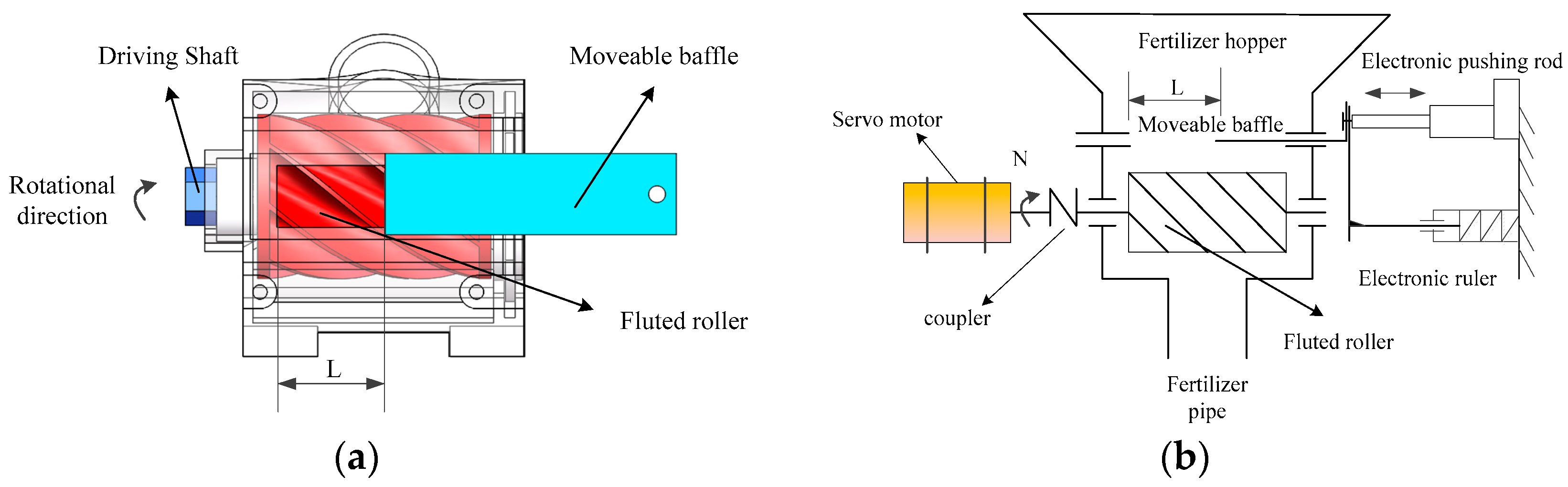
3.1. Working Principle of BFA and Data Preparation

3.1.1. Working Principle

The schematic diagram of the bivariate control mechanism for the BAF platform is presented in Figure 1. This mechanism comprises four main components: a fertilizer hopper, a device that adjusts the opening length (L), a device that adjusts the rotational speed of the fluted roller (N), and a fertilizer pipe. During operation at a specific opening length L, the fertilizers in the top of the hopper drop into the spiral fluted roller due to the gravitational force. As the shaft of the fluted roller rotates, the fertilizers are introduced into the distributor through the top entrance, ultimately falling into the fertilizer pipe under the fluted roller. As shown in Figure 1b, the L was adjusted by an electronic pushing rod connected to a moveable baffle, while the speed (N) was driven by a servo motor. Consequently, the fertilization application rate (Q) can be precisely controlled by adjusting the control parameters L and N.

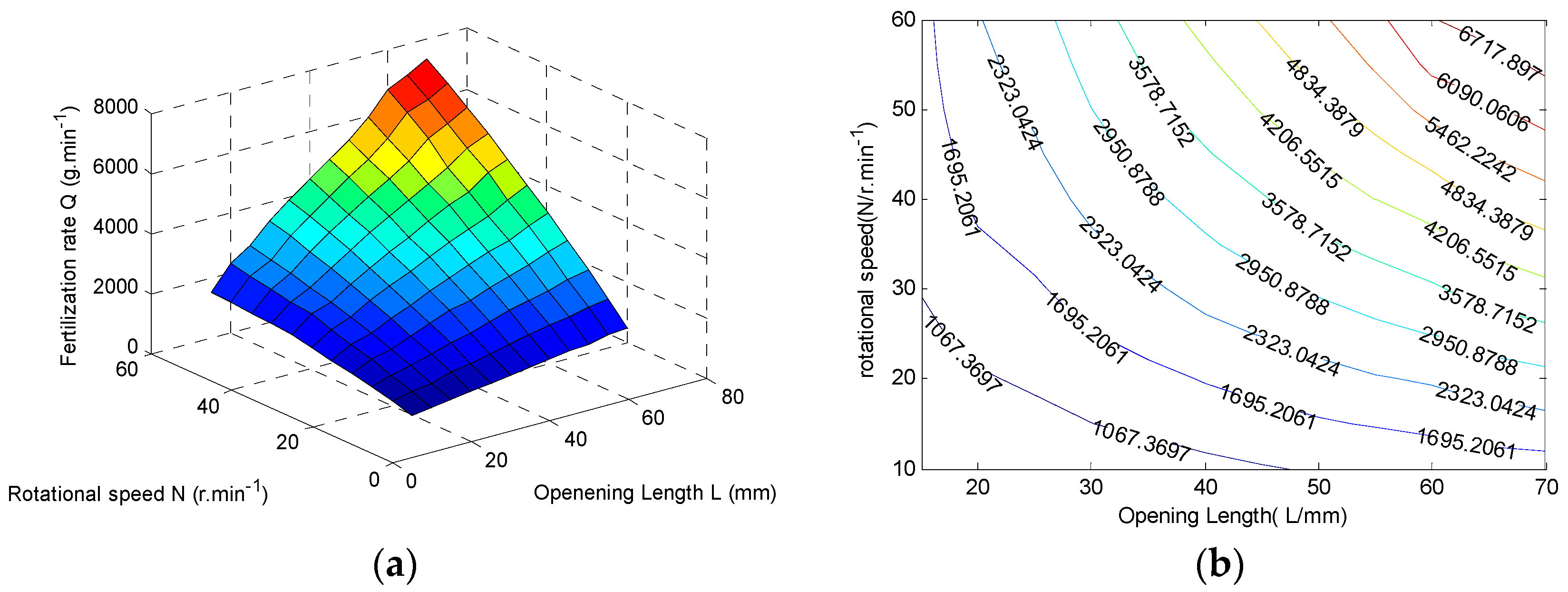
3.1.2. Data Preparation

To obtain a dataset for the CSO modeling, an indoor calibration experiment was conducted. The details are as follows: The granular fertilizer used in the tests was a compound fertilizer, with compositions of nitrogen, phosphate, and potassium at 22%, 8%, and 10%, respectively. The density of the fertilizer was 1550 kg/m³. The tests were carried out under static measurement conditions, varying the control sequences for L and N. Considering the minimum working velocity of the servo motor required to achieve stable operating conditions, L was varied from 15 to 70 mm in increments of 5 mm, while N was adjusted from 10 to 60 r/min at the same intervals. The fertilizer device was tested at specific L and N values for 1 min. The fertilizers that fell from the hopper were collected in a small bucket and weighed using a balance. Each test set was repeated three times, and the average fertilization rate per minute was calculated. A total of 132 data groups were compiled and fitted using MATLAB, as illustrated in Figure 2.

The contour map of the fertilization rate, illustrated in Figure 2b, indicates that multiple combinations of L and N can yield the same target fertilization rate. Consequently, it is essential to optimize the control sequences (L, N) for a specific fertilizer rate.

3.2. COS Problem Description and MOP Formulation

The multi-objective CSO problem for a BFA involves determining the optimal combination of L and N to achieve the desired fertilization rate while considering the fertilization accuracy, uniformity, and adjustment rapidity. The description and formulation of the three objective optimization models are as follows:

3.2.1. Accuracy Objective Function

The accuracy can be estimated by comparing the fertilizer discharge rate differential between the targeted and predicted values [33]. Based on the DFRPM by the general regression neural network (GRNN), the function can be defined as follows [9]:

$${minf}_1\left(L,N\right)=\left|{\displaystyle \frac{\left|q_p-q_t\right|}{q_t}}-\epsilon \right|,$$

(1)

where the parameter $q_p$ represents the fertilization rate, as predicted by the improved GRNN model, and is computed by Equation (5). The parameter $q_t$ represents the target fertilization rate according to the prescription map, and $\epsilon$ is the maximum allowed error of the fertilization applicator.

3.2.2. Uniformity Objective Function

Generally, the application uniformity is typically assessed through a field test and evaluated by the coefficient of variation (CV) after data processing, which is influenced by the structure of the fertilizer distributor. Our previous research indicates that for a BAF equipped with a spiral fluted roller distributor, the control sequence positions (L, N) that are close to a specific line on the contour map of the fertilization rates exhibit a smaller CV at a given target rate, indicating good fertilization uniformity [32]. Consequently, we define the minimization of the distance between control sequence position (L, N) and this line as the objective function for fertilization uniformity. The function for fertilization uniformity is presented as follows [18]:

$$min{f}_2(L,N)=\left|{\displaystyle \frac{1.15L_1-N_1-10.97}{1.524}}\right|,$$

(2)

where the L₁ (in mm) and N₁ (in revolutions/min) represent the parameters that need to be optimized, which can be represented as a control sequence matrix $S_1={(L_1,N_1)}^T$_.

3.2.3. Adjustment Rapidity Function

The adjustment rapidity refers to the minimum time required by the BAF to transition from one target fertilization rate value to another. This rapidity is related to the structure of the fertilizer distributor, and it can be detected during the fertilization process. For a BAF, since one target fertilization rate can be achieved by the control sequences L and N, we define the longer adjustment time between them as the real adjustment time. Supposing that $S_0={(L_0,N_0)}^T$ represents the previous adjustment sequence, and $S_1={(L_1,N_1)}^T$ denotes the current adjusting sequence, we define the final adjustment time to be defined as follows [18]:

$$min{f}_3\left(\mathrm{L},\mathrm{N}\right)={‖{T_{adj}(S}_0-S_1)‖}_{\infty }, T_{adj}={(t_L,t_N)}^T,$$

(3)

where $T_{adj}$ denotes the unit adjustment time, which contains the time of the opening length $t_L$ (in s/mm) and rotational speed $t_N$ (in s/revolution), which can be detected by sensors in the fertilization process.

Based on the previous analysis, Functions (1)–(3) were utilized to construct the MOP. In light of practical considerations, the control parameters L and N must be constrained within an appropriate range. The constraints for the CSO problem are defined in Equation (4) as follows:

$$\mathrm{s}.\mathrm{t}. \left\{\begin{array}{c}L\in \left[L_{\mathrm{m}\mathrm{i}\mathrm{n}},L_{\mathrm{m}\mathrm{a}\mathrm{x}}\right]\\ N\in \left[N_{\mathrm{m}\mathrm{i}\mathrm{n}},N_{\mathrm{m}\mathrm{a}\mathrm{x}}\right]\\ S_0={\left(L_0,N_0\right)}^T\\ S_1={\left(L_1,N_1\right)}^T\end{array}\right.$$

(4)

4. Evolutionary Multi-Objective Algorithms

MOEAs have been demonstrated as effective tools for identifying solutions to MOPs and have been applied in COS problems of the BAF, as mentioned above. In recent decades, several promising MOEAs, including MOEA/D-D, NSGA-III, and ar-MOEA, have been proposed. In this study, we will compare their performance on the COS problem. This section provides a brief description of these algorithms applied in this study and the performance indicators for multi-objective optimization utilized in this work.

4.1. Approaches of Evolutionary Multi-Objective Optimization

4.1.1. NSGN-III

The evolutionary multi-objective optimization algorithm based on reference-point-based non-dominated sorting (NSGA-III) was proposed by Deb and Jain [22]. NSGA-III uses the framework of the NSGA-II procedure with significant modifications in its crowding distance operator to tackle MOPs. The algorithm first classifies the population into non-dominated levels. Then, a set of reference points on a normalized hyperplane are applied to maintain diversity among the population members [28]. Each member of the population is connected to a reference point according to the vertical distance of the reference line, and the non-dominant solutions from nearby reference points are then prioritized. After generating a descending solution, the non-dominant classification method and the elite mechanism are used according to the NSGN-II program. NSGA-III has been successfully applied to multi-objective test problems with 3 to 15 objectives and has demonstrated its ability to find a representative set of solutions in various practical problems.

4.1.2. MOEA/DD

The multi-objective evolutionary algorithm based on dominance and decomposition (MOEA/DD) is proposed by Li et al. in 2015 [30]. It combines MOEA/D and NSGA-III for multi-objective optimization by leveraging the advantages of both dominance- and decomposition-based approaches. MOEA/DD decomposes a multi-objective problem into a set of scalar subproblems using a predefined weight vector [28]. The algorithm employs a steady-state update mechanism, where offspring solutions are generated through neighborhood-restricted mating (prioritizing adjacent subregions) and variation operators. Population updates follow a hierarchical strategy: firstly, solutions are sorted by Pareto dominance levels; secondly, they are evaluated via local niche counts to manage diversity; and, finally, they are optimized using scalarization functions. Notably, MOEA/DD preserves solutions in isolated subregions even if they belong to the worst nondomination level, thereby mitigating diversity loss in high-dimensional spaces. This hybrid framework effectively addresses the challenges of balancing convergence and diversity in multi-objective optimization.

4.1.3. Ar-MOEA

The multi-objective evolutionary algorithm based on preference angle and reference information was proposed by Jun Yi et al. [24]. Ar-MOEA introduces a novel dominance relation, Ar-dominance, which combines Euclidean distance and angle information between candidate solutions and reference points to evaluate the degree of convergence and population diversity. The algorithm uses an adaptive threshold to adjust the judgment condition of Ar-dominance, allowing it to dynamically balance convergence and diversity during the evolutionary process. In Ar-MOEA, the population is guided by preference information to converge toward the region of interest (ROI) specified by the decision-maker. The algorithm employs an archive to maintain a set of high-quality solutions that are closer to the reference points. The archive is updated based on the Ar-dominance relation, ensuring that the solutions retained are those that best meet the preference criteria. Through the use of adaptive weight and threshold strategies, Ar-MOEA effectively balances the trade-off between convergence and diversity, leading to improved performance in solving multi-objective optimization problems.

4.2. Performance Metrics for CSO Problem

To evaluate the performance of different MOEAs on the CSO problem for the BFA quantitative, it is crucial to define and utilize appropriate performance metrics. Unlike single-objective problems, the evaluation of results for MOPs is considerably more complex, as the outcome consists of a set of trade-off solutions pertaining to the desired objectives, which are known as non-dominated solutions according to the Pareto dominance concept [34]. Convergence and coverage of the solutions are the main aspects concerned by most MOPs [35]. In the case of the CSO-MOP, an exact optimal PS cannot be identified; therefore, indicators such as inverted generational distance (IGD) and generational distance (GD) are inapplicable [36]. Instead, we employ the hypervolume (HV) and spacing (SP) indicators to evaluate the convergence and coverage. Additionally, as this is a practical problem, computing time is also essential, as it constrains the application of this technology. Consequently, the runtime (RT) for each algorithm’s computing process needs to be recorded in this paper. The details of these metrics are as follows:

4.2.1. Hypervolume (HV)

HV represents the volume of the objective space covered by the identified PF, serving as a crucial metric for assessing the convergence behavior of MOEAs. Specifically, a larger HV value indicates that the solutions from the PS are more evenly distributed within the objective space. It is important to note that a reference point is required to compute the covered space.

4.2.2. Spacing (SP)

The spacing (SP) of the objective space covered by the obtained PF is a crucial metric for evaluating the variance of the PF. A lower SP value indicates a greater number of solutions that are more evenly distributed along the Pareto optimal front. The mathematical expression for SP is presented as follows:

$$SP\triangleq \sqrt{{\displaystyle \frac{1}{n-1}}{\sum }_{i=1}^n{(\overline{d}-d_i)}^2}$$

(5)

where $\overline{d}$ is the average of all $d_i$, and $n$ is the number of Pareto optimal solutions obtained [35].

4.2.3. Running Time (RT)

Running time (RT) denotes the total time required for an algorithm to be executed, reflecting its computational efficiency. Under identical conditions, a shorter running time indicates a higher computational efficiency. In the context of CSO-MOP, which is an agricultural application, a reduced runtime of the algorithm can facilitate the implementation of the BAF. Therefore, this paper utilizes RT as the metric for assessing the computational efficiency of the MOEAs discussed in this paper.

5. Computational Experiments

In this section, test experiments are designed to evaluate the performance of the MOEAs, including NSGA-III [37], MOEA/D-D [30], and Ar-MOEA [24], on the CSO problem for the BAF.

5.1. Experimental Design

Considering the actual fertilization requirement, a total of six target fertilization rate $q_t$ values ranging from 150 kg/ha to 400 kg/ha, with an interval of 50 kg/ha, were selected as the test instance. The control sequence considering the fertilization accuracy, uniformity, and equipment adjusting rapidity at each $q_t$ was optimized by the three MOEAs mentioned above.

The experiments are conducted using a computing system equipped with the Windows 11 operating system, 32 GB of RAM, and an Intel (R) Core (TM) i9-12900 H CPU (2.40 GHz). The comparison methods are coded using MATLAB R2023a. Each instance is run 30 times independently for the three comparison algorithms. The basic parameters of the CSO problem and the algorithms are provided in the remainder of this section.

5.2. Parameter Settings

In this section, we introduce the necessary parameter settings for solving the CSO problem. Before the computing tests, the DFRPM were trained by GRNN, and the net data were prepared in advance. Other parameter values required by the CSO problem are shown in

Table 2. The CSO problem model parameter setting.

Parameter	Value	Unit
Target fertilization rate (Qt)	[150,200,250,300,350,400]	kg/ha
Range of the active feed-roll length (L)	[15,70]	mm
Range of the rotational speed of driving shaft (N)	[10,60]	r/min
Previous adjustment sequence (S0)	[35,0]T	[mm, r/min]T
Allowance error (ε)	0.01	-
Unit adjusting time (Tadj)	[0.15,0.025]T	[s/mm, s/(r/min)]T

.

It is necessary to initialize the basic parameters of the algorithm before computing. For a fair comparison, all algorithms are considered with 50 iterations, and the population size is established by the number of subproblems decomposed by MOEA/D-D. These decomposed subproblems are formulated by a set of weight vectors, which are generated by the simplex-lattice design using H = 20. Consequently, the population size N was set as N = 231. Other parameters, such as the step size for Ar-MOEA and the number of weight vectors, were kept at their default values.

Once the parameters mentioned above were determined, the optimization process was conducted in MATLAB. Finally, the solution set of the consequences (PS) and results of the objective functions (PF) at a specific target fertilization rate can be identified. For MOEAs based on decomposition, such as NSGA-III and MOEAD-D, the appropriate selection of parameters (L, N) can be obtained by selecting a weight vector that aligns with the practical needs, as each weight vector corresponds to a specific control sequence (L, N) in the Pareto set.

5.3. Evaluation Criteria

The selection of metrics is crucial for a comprehensive analysis of the MOEAs on the CSO-MOP. Three aspects must be considered when analyzing the performance of these algorithms: firstly, the algorithm performance in solving the CSO-MOP; secondly, the conflicts between every pair of objectives; and thirdly, the effects of the optimized control sequences. Consequently, the metrics utilized in these areas are selected as follows:

5.3.1. Criteria for the Performance of the MOEAs

To evaluate the performance of the three MOEAs on CSO-MOP, two aspects must be considered: the quality of the results and the solving speed. As discussed in Section 4.2, the convergence and coverage of the PS are the primary concerns for most MOPs, while the RT is also critical for practical applications. Therefore, the performance of the MOEAs on the CSO-MOP is assessed using indicators such as HV, SP, and RT.

When calculating the HV index, the selection of the approximated front (approx. Front) directly affects the fairness and accuracy of the evaluation results. In our experiments, the approx. Front that all three algorithms found at the end of the 30 executions was constructed. The reference vector was computed by covering the largest value for each objective function in the Pareto reference set and increasing its magnitude by 10%. Based on the approx. Front, the SP of the three algorithms at different fertilization rates was calculated.

5.3.2. Criteria for the Conflict Analysis Between Different Objectives

Parallel coordinates are frequently employed to visualize correlations among objectives [38], where the objectives are normalized within the range of [0, 1]. Lines are traced between adjacent objectives to highlight the correlation between pairs of consecutive objectives. If two polylines frequently intersect in specific regions, this indicates a conflict between the corresponding objectives; conversely, if the polylines remain relatively parallel, it suggests a higher degree of consistency among the corresponding objectives.

The Pearson correlation coefficient quantifies the linear relationship between two objectives, with values ranging from −1 to 1. Utilizing a correlation coefficient matrix enables the quantification of correlations among the targets. A coefficient near 1 signifies a strong positive correlation, while a coefficient near −1 indicates a strong negative correlation; that is, if one objective value decreases, the other increases. A coefficient close to 0 suggests the absence of a linear correlation between the objectives.

Therefore, we use the Pearson correlation coefficients as the metric to numerically analyze the linear relationships among the three objectives and create parallel coordinates to visualize correlations among these three different objectives.

5.3.3. Criteria for the Performance of Optimized Control Sequence on Three Objectives

The performance of the MOEAs on CSO-MOP is ultimately reflected by the impact of the optimized control sequence on the three objectives: fertilization accuracy, uniformity, and adjusting time. Therefore, a specific weight vector of (0.9, 0.05, 0.05) was selected, where the accuracy objective is assigned a weight of 90%, the uniformity objective is assigned a weight of 5%, and the adjustment rapidity objective is assigned a weight of 5%. The objective results at the weight vector of (0.9, 0.05, 0.05) from the MOEAs, including fertilization accuracy, uniformity, and adjustment time, were finally compared.

According to the definition of the CSO problem, the fertilization accuracy can be estimated by comparing the differences between the targeted and predicted fertilizer discharge rate. Consequently, the relevant error (RE) is selected as the metric for evaluating the fertilization accuracy [9]. The function of the RE is computed as follows:

$$\mathrm{R}\mathrm{E}={\displaystyle \frac{\left|y_{tar}-y_{pre}\right|}{y_{tar}}}\times 100\%$$

(6)

where $y_{tar}$ is the target rate that needs to be applied (kg/ha), and $y_{pre}$ is the predicted discharge rate (kg/ha) at the optimized control sequence. Lower values of $\mathrm{R}\mathrm{E}$ indicate higher accuracy of the system.

In this paper, application uniformity is defined as the distance from the position of the optimized control sequence to a specific line on the contour map of the fertilization rates. A smaller distance indicates better application uniformity. Consequently, fertilization uniformity is calculated as shown in Equation (2), and the value of the uniformity objective ($F_2$) at the optimized control sequence is used as a metric to evaluate the fertilization uniformity.

We define the adjustment rapidity as the minimum time required for the BAF to transition from one target fertilization rate value to another. Therefore, the minimum adjustment time value ($F_3$) from the initial control sequence (L = 35 mm, N = 0 r/min) to the optimized control sequence is calculated, as shown in Equation (3), as a metric to evaluate the adjustment rapidity.

6. Results and Discussion

6.1. Performance Comparison of MOEAs

To evaluate the performance of the three MOEAs, we summarize the performance indicators, including hypervolume (HV), spacing (SP), and runtime (RT), as applied to the results obtained by NSGA-III, MOEA/D-D, and Ar-MOEA for the test instances ranging from 150 kg/ha to 400 kg/ha in Table 2. This table consists of four main columns: the first column corresponds to the test instance, while the subsequent three columns represent the performance metrics for NSGA-II, SMS-EMOA, and MOEA/D, respectively. Each algorithm has three associated columns that indicate the HV, SP, and RT values. For each test instance, algorithm, and performance metric, we present both the average value of the performance indicator and its corresponding standard deviation. To facilitate a clear visualization of the optimal values for each performance indicator and test instance, these values are highlighted in boldface.

As shown in

Table 3. Summary of the HV, SP, and RT performance indicators.

MOP	NSGA-III			MOEAD/D			AR-MOEA
Qt/Kg.ha−1	HV	SP	RT/s	HV	SP	RT/s	HV	SP	RT/s
150	1.64 ± 3.56 × 10−2	7.52 × 10−1 ± 1.98 × 10−2	5.57 × 10 ± 5.71	1.67 ± 1.04 × 10−3	1.14 ± 1.94 × 10−3	1.84 × 10 ± 7.97 × 10−2	1.64 ± 7.58 × 10−5	7.21× 10−1 ± 9.82 × 10−3	8.76 × 10 ± 3.86
200	8.24 × 10−1 ± 5.14 × 10−2	1.32 ± 1.01 × 10−1	8.13 × 10 ± 8.85	8.19 × 10−1 ± 1.31 × 10−3	1.05 ± 4.21 × 10−3	1.94 × 10 ± 5.79	7.91 × 10 ± 1.01 × 10−3	7.46 ± 2.23 × 10−2	8.09 × 10 ± 4.01
250	1.30 ± 1.89 × 10−1	7.90 × 10−1 ± 4.37 × 10−2	1.25 × 102 ± 8.79	1.15 ± 1.57 × 10−2	1.08 ± 4.90 × 10−3	1.93 × 10 ± 5.08 × 10−1	1.07 ± 1.29 × 10−2	7.27 × 10−1 ± 1.16 × 10−2	7.74 × 10 ± 2.51
300	2.21 ± 4.64 × 10−2	8.95 × 10−1 ± 6.30 × 10−2	1.45 × 102 ± 8.26	2.09 ± 1.75 × 10−2	1.14 ± 4.45 × 10−3	1.86 × 10 ± 6.89 × 10−2	1.78 ± 2.30 × 10−2	7.13 × 10−1 ± 4.05 × 10−3	8.25 × 10 ± 3.06
350	2.02 ± 4.50 × 10−2	7.67 × 10−1 ± 2.42 × 10−2	1.64 × 102 ± 1.92 × 10	1.09 ± 3.08 × 10−2	1.12 ± 7.61 × 10−3	1.87 × 10 ± 3.97 × 10−1	1.64 ± 3.68 × 10−2	7.08 × 10−1 ± 6.87 × 10−3	8.53 × 10 ± 2.93
400	1.94 ± 6.02 × 10−2	7.70 × 10−1 ± 2.84 × 10−2	1.71 × 102 ± 5.34	1.85 ± 3.43 × 10−2	1.11 ± 6.67 × 10−3	1.83 × 10 ± 5.75 × 10−2	1.63 ± 2.93 × 10−2	6.97 × 10−1 ± 3.51 × 10−3	8.46 × 10 ± 2.78

, NSGA-III demonstrates superior performance over the other two algorithms in terms of the HV metric, which can be attributed to its symmetric reference point distribution, which mirrors the rotational symmetry in the BFA’s control parameter space. Conversely, the asymmetric search bias of MOEA/D-D leads to localized convergence, sacrificing global symmetry preservation for computational efficiency. While in terms of the SP metric, Ar-MOEA exhibited statistically significant superiority over both NSGA-III and MOEAD-D across all experimental instances. Interestingly, while MOEAD-D generally displayed the poorest SP performance, it unexpectedly outperformed NSGA-III at the 200 kg/ha fertilization level while still maintaining higher overall SP values compared to the other algorithms. Conversely, MOEAD-D required substantially less computational time (RT) than the other algorithms, with a mean runtime of 18.5 ± 0.5 s across the test instances, whereas NSGA-III and Ar-MOEA required approximately 125 and 85 s, respectively.

To better analyze the impact of the target fertilization rate (Qt) on the performance of these three algorithms, we constructed a line chart (Figure 3) using the data presented in Table 2.

As illustrated in Figure 3a, the HV value exhibits a trend of initially decreasing and subsequently increasing with the rise in Qt. Specifically, at the first Qt point (150 kg/ha), the HV values for all three algorithms approximate 1.65. At the second Qt point (200 kg/ha), the HV reaches its minimum (approximately 0.8). Ultimately, as Qt continues to increase, the HV gradually rises, achieving its maximum value at the fourth Qt point (300 kg/ha). Regarding the SP metrics, Figure 3b indicates that variations in Qt have a minimal impact on the performance of the MOEAD-D and Ar-MOEA algorithms, with the exception of NSGA-III, which exhibits a notable change at Qt of 200 kg/ha. Similar results are reflected for the RT metrics, as shown in Figure 3c, where the RT metrics remain stable with changes in Qt for MOEAD-D and Ar-MOEA. Conversely, for NSGA-III, the RT increases in correlation with the Qt value. This may be attributed to the fact that the NSGA-III algorithm requires non-dominated sorting and reference point association in each generation, resulting in a computational complexity that is directly proportional to the evaluation time of Qt. In contrast, the MOEA/D-D algorithm, which is based on decomposition, typically relies on local information to optimize each subproblem, leading to a runtime that remains unaffected by increases in Qt. Similarly, the AR-EMOA utilizes an adaptive mechanism to dynamically adjust the evaluation frequency, thereby minimizing redundant computations and mitigating the additional operational time incurred by an increase in Qt.

In summary, regarding the convergence and coverage of the solutions, NSGA-III demonstrates superior performance. However, in practical applications, the MOEAD-D algorithm maintains a commendable level of convergence and coverage within the PS while achieving the shortest computation time, thereby enhancing its value for practical use.

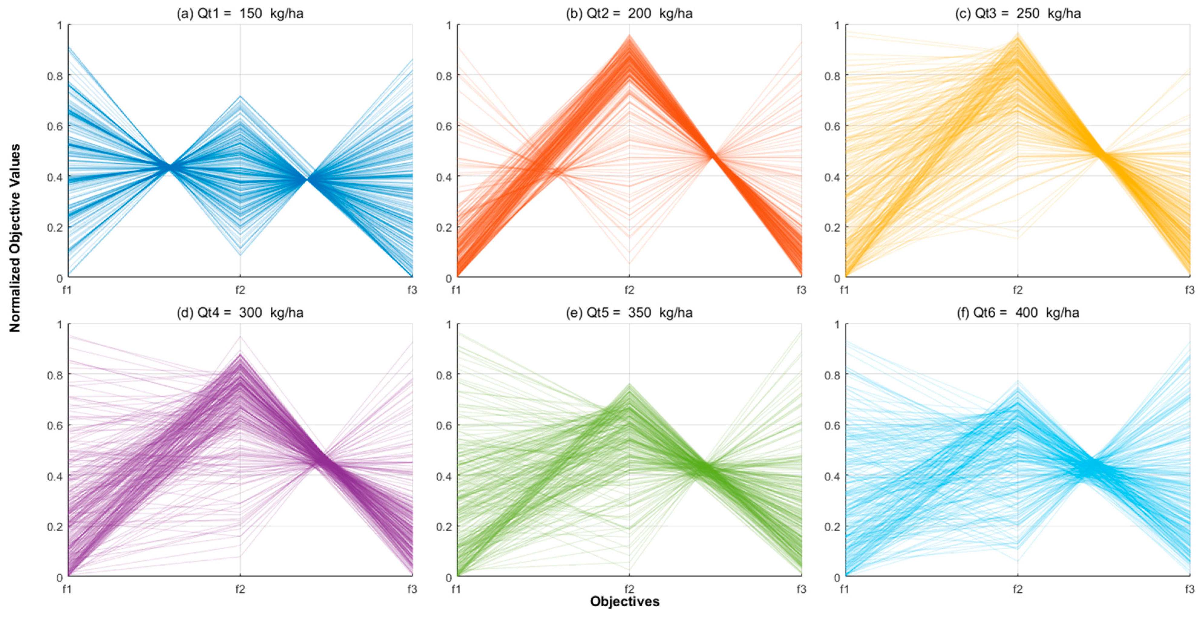
6.2. Analysis of the Conflict Between Different Objects

In this section, we investigate the conflict between different objectives by employing parallel coordinates of the Pareto reference set alongside Pearson correlation coefficients to quantify the results. A PS characterized by superior diversity and convergence can more comprehensively cover the Pareto front, thereby providing a more accurate reflection of the relationships among the objectives. As analyzed in Section 6.1, the solution set derived from the NSGA-III algorithm typically demonstrates enhanced diversity and convergence. Consequently, we utilize the solution set obtained from the NSGA-III algorithm to analyze the relationships among the three objectives.

To ensure the reliability of the correlation analysis among multiple objectives, we combined the results from 30 runs of the NSGA-III algorithm and performed non-dominated sorting to obtain a comprehensive non-dominated PF that covers the global scope. To enhance the validity and representativeness of the data while improving the running efficiency, we employed a stratified sampling method and visualized the data using parallel coordinate plots, as illustrated in Figure 4.

We illustrate the conflict between pairs of objectives for the problem, with a target fertilization rate (Qt) ranging from 150 kg/ha to 400 kg/ha at intervals of 50 kg/ha, as depicted in Figure 4. Notably, a symmetric correlation exists between objectives $f_1$ versus $f_2$ and $f_2$ versus $f_3$ at a target fertilization rate (Qt) of 150 kg/ha and an asymmetric correlation between them at other Qt. In Figure 4a, the objectives between $f_1$ and $f_2$, as well as $f_2$ and $f_3$, exhibit a negative correlation, suggesting that optimizing one objective results in the deterioration of the other. Conversely, at other target fertilization rates, as shown in Figure 4b–f, the intersections between objectives $f_1$ versus $f_2$ gradually decrease. This suggests that as Qt increases, the correlation between objectives $f_1$ and $f_2$ becomes less significant. However, the comparison between $f_1$ versus $f_3$ is not straightforward.

To analyze the objective correlation in the Pareto reference sets numerically, we calculate the Pearson correlation coefficients between the pairs of objectives for both problem formulations and present the results in Figure 5. As illustrated in Figure 5, a similar relationship between objectives $f_1$ and $f_2$ is observed. At a target fertilization rate (Qt) of 150 kg/ha, a strong negative correlation is evident, with a coefficient of −1. As the Qt increases, the coefficient decreases, ultimately approaching zero, indicating that as Qt rises, the correlation diminishes and eventually becomes non-existent. In contrast, a strong negative correlation exists between objectives $f_2$ and $f_3$, with the nearing −1. The relationship between objectives $f_1$ and $f_3$ is more complex. Specifically, in Figure 5a, at Qt = 150 kg/ha, the coefficient is approximately 1 (0.99), indicating an extremely strong positive correlation. However, at Qt = 200 kg/ha in Figure 5b, the coefficient decreases to 0.78, signifying a strong positive correlation. As shown in Figure 5c, the coefficient further decreases to −0.33 at Qt = 250 kg/ha, indicating a weak negative correlation between objectives $f_1$ and $f_3$. Subsequently, the coefficient stabilizes around −0.2, suggesting a lack of correlation between these objectives.

In summary, a strong negative correlation exists between objectives $f_2$ and $f_3$. The relationships between $f_1$ and $f_2$, as well as $f_1$ and $f_3$, are influenced by the target fertilization rate (Qt). At Qt of 150 kg/ha and 200 kg/ha, a strong negative correlation is observed between $f_1$ and $f_2$, while a strong positive correlation exists between $f_1$ and $f_3$. However, at Qt exceeding 250 kg/ha, the correlation between these objectives disappears. This result can provide guidance for the selection of control sequences during actual operations. For instance, at low target rates (Qt < 250 kg/ha), the strong negative correlation between accuracy ($f_1$) and uniformity ($f_2$) indicates a strict trade-off. To achieve balance, the control sequence should prioritize accuracy, while at higher target rates (Qt > 250 kg/ha), a weakened correlation allows for greater flexibility. In this context, dynamic weight adaptation can be implemented to adjust objective priorities based on practical needs. The recommended proper fertilization rate typically falls below 250 kg/ha, indicating that both positive and negative correlations between pairs of objectives exist in the CSO-MOP problems. The varying correlations among objectives determine the shape of the Pareto surface [39]. Specifically, when both positive and negative correlations among objectives are present, they can produce a degenerated surface, thereby complicating the problem for multi-objective optimization solvers.

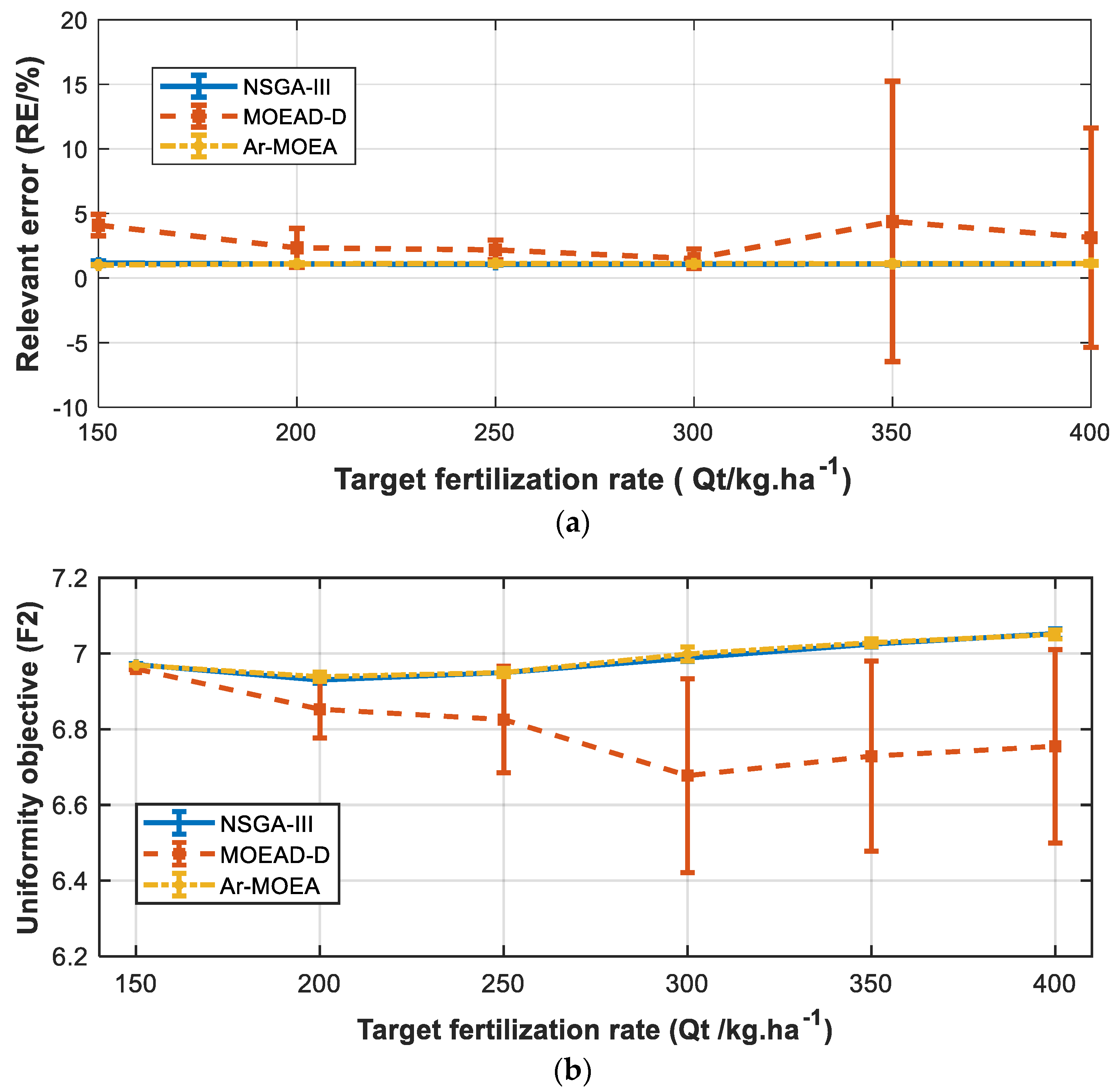
6.3. Performance on CSO-MOP

To evaluate the performance of the three MOEAs on the COS-MOP, we present the performance of these algorithms by focusing on the optimization of each objective and its relation to the target fertilization rate (Qt). In variable-rate fertilization, fertilization accuracy is a crucial element that must be considered; therefore, a weight vector of (0.90, 0.05, 0.05) was chosen, with the accuracy objective assigned a weight of 90%. The fertilization metrics mentioned in Section 5.3.3 are calculated and summarized in

Table 4. Summary of the fertilization performance metrics obtained by the MOEAs.

MOP	NSGA-III			MOEAD/D			AR-MOEA
Qt/Kg.ha−1	RE/%	F2	F3	RE/%	F2	F3	RE/%	F2	F3
150	1.15 ± 1.76 × 10−1	6.97 ± 2.32 × 10−3	5.11 × 10−1 ± 1.24 × 10−2	4.10 ± 0.83× 10−1	6.95 ± 2.33 × 10−3	3.99 × 10−1 ± 2.60 × 10−2	1.01 ± 1.33 × 10−2	6.97 ± 1.25 × 10−2	3.18 × 10−1 ± 2.16 × 10−2
200	1.09 ± 7.06 × 10−2	6.93 ± 3.56 × 10−2	3.12 × 10−1 ± 9.28 × 10−3	2.34 ± 1.50 × 10−2	6.85 ± 7.61 × 10−2	9.95 × 10−1 ± 6.55 × 10−1	1.10 ± 9.08 × 10−2	6.94 ± 1.25 × 10−2	3.18 × 10−1 ± 2.16 × 10−2
250	1.07 ± 4.92 × 10−2	6.95 ± 4.41 × 10−3	3.69 × 10−1 ± 7.40 × 10−3	2.18 ± 7.61 × 10−1	6.83 ± 1.41 × 10−1	1.46 ± 1.35	1.13 ± 1.02 × 10−1	6.95 ± 1.06 × 10−2	3.89 × 10−1 ± 1.95 × 10−2
300	1.07 ± 7.45 × 10−2	6.99 ± 4.41 × 10−3	4.57 × 10−1 ± 2.14 × 10−2	1.50 ± 7.53 × 10−1	6.67 ± 2.56 × 10−1	3.30 ± 2.38	1.11 ± 1.09 × 10−1	6.70 ± 1.84 × 10−2	4.55 × 10−1± 1.00 × 10−2
350	1.08 ± 8.02 × 10−2	7.02 ± 7.88 × 10−3	5.46 × 10−1 ± 1.93 × 10−2	4.38 ± 1.09 × 10	6.73 ± 2.51 × 10−1	2.98 ± 2.32	1.11 ± 8.07 × 10−2	7.29 ± 1.01 × 10−2	5.47 × 10−1 ± 1.60 × 10−2
400	1.11 ± 1.08 × 10−3	7.05 ± 1.29 × 10−2	5.87 × 10−1 ± 1.40 × 10−2	3.12 ± 8.49 × 10−2	6.76 ± 2.55 × 10−1	2.92 ± 2.29	1.14 ± 1.35 × 10−1	7.05 ± 1.21 × 10−2	5.93 × 10−1 ± 2.09 × 10−2

. The fertilization performance metrics, including RE, $F_2$, and $F_3$ values, at different target fertilization rates were calculated for each algorithm, with the best values for each subjective indicator indicated in boldface.

The performance metrics mentioned in Section 5.3.3 for NSGA-II, SMS-EMOA, and MOEA/D are summarized and shown in Table 3. Each algorithm has three associated columns that indicate the RE, F2, and F3 values. For each test instance, algorithm, and performance metric, we present both the average value of the performance indicator and its corresponding standard deviation.

To facilitate a clear visualization, the optimal values are highlighted in boldface, and a line chart based on the data presented in Table 4 is plotted in Figure 6.

Figure 6 illustrates that NSGA-III and Ar-MOEA exhibit similar trends in terms of fertilization accuracy, uniformity, and adjustment rapidity, while the results from MOEAD-D fluctuate based on the target fertilization rate (Qt). Specifically, regarding the fertilization accuracy, as depicted in Figure 6a, NSGA-III and Ar-MOEA demonstrate better performance in the RE metric, with RE values consistently below 2%. In contrast, the RE value for MOEAD-D remains below 5%, which is acceptable according to the relevant national standards. The application uniformity objective ($F_2$) values from MOEAD-D significantly outperform those of the other two algorithms, with $F_2$ values below 7. Conversely, the $F_2$ values for NSGA-III and Ar-MOEA are approximately 7. Regarding the adjustment rapidity ($F_3$), NSGA-III and Ar-MOEA show lower adjustment times, averaging around 0.5 s. In contrast, the adjustment time from MOEAD-D increases with the target fertilization rate (Qt), rising from 0.4 s to 3 s.

In summary, while the results from NSGA-III and MOEAD-D exhibited better performance compared to MOEAD-D in terms of fertilization accuracy and adjustment speed, it is important to note that MOEAD-D still maintains acceptable levels of fertilization accuracy and demonstrates better uniformity.

7. Conclusions

In this study, we examined the CSO problem as a multi-objective problem with three objectives for BFA. To achieve a balance between the solution accuracy and efficiency, we employed three MOEAs, NSGA-III, MOEAD-D, and AR-MOEA, and conducted a comparative analysis. We considered three aspects: the performance of each algorithm in addressing the CSO-MOP, the conflicts between each pair of objectives, and the effects of the optimized control sequences obtained from each algorithm on the three objectives. Experiments were conducted under the same conditions, and the appropriate metrics were selected. The conclusion is summarized as follows:

Firstly, regarding algorithm performance, our findings suggest that the PS from NSGA-III and Ar-MOEA demonstrates better convergence and coverage at the cost of longer computing times compared to MOEAD-D. Secondly, both positive and negative correlations exist between the pairs of objectives in the CSO-MOP problems, indicating a degenerated surface of the PF. This suggests that the CSO-MOP problem cannot be effectively addressed by merely merging it into a single-objective optimization problem using the weighted sum method. Finally, concerning the performance of the algorithms on each objective, all three algorithms can optimize each objective and obtain reasonable results. Specifically, the results from NSGA-III and MOEAD-D exhibited better performance in terms of fertilization accuracy and adjustment speed, while MOEAD-D maintained acceptable levels of fertilization accuracy and demonstrated better uniformity. Therefore, NSGA-III and Ar-MOEA are more suitable for off-line optimization, such as pre-computing Pareto sets for known prescription maps, rather than for real-time control. In contrast, MOEA/D-D demonstrates potential for near-real-time applications, as its runtime of around 18.4 s is more aligned with the operational requirements for real-time applications, where control sequences need to be updated every 15 s (e.g., 20 m × 20 m grid resolution at a vehicle speed of 5 km/h). However, there are still challenges to address, such as the need for further acceleration of the algorithm, hardware limitations, and dynamic environmental changes, like vibrations, which must be overcome in the future.

Given the interesting results obtained in this research, it is indispensable to investigate the conflict among additional objectives, such as the breakage rate of granular fertilizer during processing. In this paper, the CSO-MOP was solved in an off-line condition; thus, an examination can be performed in order to apply MOEAD-D to a dynamic condition in the future. Additionally, a full-factorial sensitivity analysis of key algorithm parameters (e.g., mutation rate, population size, weight vectors) of different algorithms could further enhance individual performance in the future.

References

1. Beneduzzi, H.M.; de Souza, E.G.; Moreira, W.K.O.; Sobjak, R.; Bazzi, C.L.; Rodrigues, M. Fertilizer Recommendation Methods for Precision Agriculture—A Systematic Literature Study. Eng. Agric. 2022, 42. [Google Scholar] [CrossRef]
2. Al-Gaadi, K.A.; Tola, E.K.; Alameen, A.A.; Madugundu, R.; Marey, S.A.; Zeyada, A.M.; Edrris, M.K. Control and Monitoring Systems Used in Variable Rate Application of Solid Fertilizers: A Review. J. King Saud Univ.-Sci. 2023, 35, 102574. [Google Scholar] [CrossRef]
3. Pramod Pawase, P.; Madhukar Nalawade, S.; Balasaheb Bhanage, G.; Ashok Walunj, A.; Bhaskar Kadam, P.; Durgude, A.G.; Patil, M.R. Variable Rate Fertilizer Application Technology for Nutrient Management: A Review. Int. J. Agric. Biol. Eng. 2023, 16, 11–19. [Google Scholar] [CrossRef]
4. Song, C.; Zhou, Z.; Zang, Y.; Zhao, L.; Yang, W. Variable-Rate Control System for UAV-Based Granular Fertilizer Spreader. Comput. Electron. Agric. 2021, 180, 105832. [Google Scholar] [CrossRef]
5. Alameen, A.A.; Al-Gaadi, K.A.; Tola, E.K. Development and Performance Evaluation of a Control System for Variable Rate Granular Fertilizer Application. Comput. Electron. Agric. 2019, 160, 31–39. [Google Scholar] [CrossRef]
6. Chen, C.; He, P.; Zhang, J.; Li, X.; Ren, Z.; Zhao, J.; He, J.; Wang, Y.; Liu, H.; Kang, J. A Fixed-Amount and Variable-Rate Fertilizer Applicator Based on Pulse Width Modulation. Comput. Electron. Agric. 2018, 148, 330–336. [Google Scholar] [CrossRef]
7. Yang, S.; Wang, X.; Zhai, C.; Dou, H.; Gao, Y.; Zhao, C. Design and Test on Variable Rate Fertilization System Supporting Seeding and Fertilizing Monitoring. Trans. Chin. Soc. Agric. Mach. 2018, 49, 145–153. [Google Scholar] [CrossRef]
8. Liu, C.; Yuan, J.; Liu, J.; Li, C.; Zhou, Z.; Gu, Y. ARM and DSP-Based Bivariable Fertilizing Control System Design and Implementation. J. Agric. Mach. 2010, 2, 233–236. [Google Scholar]
9. Zhang, J.; Liu, G.; Luo, C.; Hu, H.; Huang, J. MOEA/D-DE Based Bivariate Control Sequence Optimization of a Variable-Rate Fertilizer Applicator. Comput. Electron. Agric. 2019, 167, 105063. [Google Scholar] [CrossRef]
10. Maleki, M.R.; Mouazen, A.M.; De Ketelaere, B.; Ramon, H.; De Baerdemaeker, J. On-the-Go Variable-Rate Phosphorus Fertilisation Based on a Visible and near-Infrared Soil Sensor. Biosyst. Eng. 2008, 99, 35–46. [Google Scholar] [CrossRef]
11. Zhang, J.; Liu, G.; Huang, J.; Zhang, Y. A Study on the Time Lag and Compensation of a Variable-Rate Fertilizer Applicator. Appl. Eng. Agric. 2021, 37, 43–52. [Google Scholar] [CrossRef]
12. Chelladurai, S.J.S.; Murugan, K.; Ray, A.P.; Upadhyaya, M.; Narasimharaj, V.; Gnanasekaran, S. Optimization of Process Parameters Using Response Surface Methodology: A Review. Mater. Today Proc. 2020, 37, 1301–1304. [Google Scholar] [CrossRef]
13. Yuan, J.; Liu, C.L.; Li, Y.M.; Zeng, Q.; Zha, X.F. Gaussian Processes Based Bivariate Control Parameters Optimization of Variable-Rate Granular Fertilizer Applicator. Comput. Electron. Agric. 2010, 70, 33–41. [Google Scholar] [CrossRef]
14. Bai, J.; Tian, M.; Li, J. Control System of Liquid Fertilizer Variable-Rate Fertilization Based on Beetle Antennae Search Algorithm. Processes 2022, 10, 357. [Google Scholar] [CrossRef]
15. Dang, Y.; Ma, H.; Wang, J.; Zhou, Z.; Xu, Z. An Improved Multi-Objective Optimization Decision Method Using NSGA-III for a Bivariate Precision Fertilizer Applicator. Agriculture 2022, 12, 1492. [Google Scholar] [CrossRef]
16. Chen, M.; Lu, W.; Wang, X.; Sun, G.; Zhang, Y. Design and Experiment of Optimization Control System for Variable Fertilization in Winter Wheat Field Based on Fuzzy PID. Trans. Chin. Soc. Agric. Mach. 2016, 47, 71–76. [Google Scholar] [CrossRef]
17. Su, N.; Xu, T.; Song, L.; Wang, R.; Wei, Y. Variable Rate Fertilization System with Adjustable Active Feed-Roll Length. Int. J. Agric. Biol. Eng. 2015, 8, 19–26. [Google Scholar] [CrossRef]
18. Zhang, J.; Liu, G. Effects of Control Sequence Optimisation on the Performance of Bivariate Fertiliser Applicator. Comput. Electron. Agric. 2022, 192, 106594. [Google Scholar] [CrossRef]
19. Başar, G.; Der, O. Multi-Objective Optimization of Process Parameters for Laser Cutting Polyethylene Using Fuzzy AHP-Based MCDM Methods. Proc. Inst. Mech. Eng. 2025, 2–15. [Google Scholar] [CrossRef]
20. Kilic, M.; Anac, S. Multi-Objective Planning Model for Large Scale Irrigation Systems: Method and Application. Water Resour. Manag. 2010, 24, 3173–3194. [Google Scholar] [CrossRef]
21. Zheng, Y.J.; Song, Q.; Chen, S.Y. Multiobjective Fireworks Optimization for Variable-Rate Fertilization in Oil Crop Production. Appl. Soft Comput. J. 2013, 13, 4253–4263. [Google Scholar] [CrossRef]
22. Deb, K.; Jain, H. An Evolutionary Many-Objective Optimization Algorithm Using Reference-Point-Based Nondominated Sorting Approach, Part I: Solving Problems with Box Constraints. IEEE Trans. Evol. Comput. 2014, 18, 577–601. [Google Scholar] [CrossRef]
23. Zhang, Q.; Li, H. MOEA/D: A Multiobjective Evolutionary Algorithm Based on Decomposition. IEEE Trans. Evol. Comput. 2007, 11, 712–731. [Google Scholar] [CrossRef]
24. Yi, J.; Bai, J.; He, H.; Peng, J.; Tang, D. Ar-MOEA: A Novel Preference-Based Dominance Relation for Evolutionary Multiobjective Optimization. IEEE Trans. Evol. Comput. 2019, 23, 788–802. [Google Scholar] [CrossRef]
25. Lanza-Gutierrez, J.M.; Gomez-Pulido, J.A. Assuming Multiobjective Metaheuristics to Solve a Three-Objective Optimisation Problem for Relay Node Deployment in Wireless Sensor Networks. Appl. Soft Comput. J. 2015, 30, 675–687. [Google Scholar] [CrossRef]
26. Trivedi, A.; Srinivasan, D.; Sanyal, K.; Ghosh, A. A Survey of Multiobjective Evolutionary Algorithms Based on Decomposition. IEEE Trans. Evol. Comput. 2017, 21, 440–462. [Google Scholar] [CrossRef]
27. Xu, Y.; Ding, O.; Qu, R.; Li, K. Hybrid Multi-Objective Evolutionary Algorithms Based on Decomposition for Wireless Sensor Network Coverage Optimization. Appl. Soft Comput. J. 2018, 68, 268–282. [Google Scholar] [CrossRef]
28. Li, K.; Wang, R.; Zhang, T.; Ishibuchi, H. Evolutionary Many-Objective Optimization: A Comparative Study of the State-of-The-Art. IEEE Access 2018, 6, 26194–26214. [Google Scholar] [CrossRef]
29. Xu, G.; Guan, Z.; Yue, L.; Mumtaz, J.; Liang, J. Modeling and Optimization for Multi-Objective Nonidentical Parallel Machinging Line Scheduling with a Jumping Process Operation Constraint. Symmetry 2021, 13, 1521. [Google Scholar] [CrossRef]
30. Li, K.; Deb, K.; Zhang, Q.; Kwong, S. An Evolutionary Many-Objective Optimization Algorithm Based on Dominance and Decomposition. IEEE Trans. Evol. Comput. 2015, 19, 694–716. [Google Scholar] [CrossRef]
31. Pu, X.; Xu, Y.; Fu, Y. Integrated Scheduling of Picking and Distribution of Fresh Agricultural Products for Community Supported Agriculture Mode. Symmetry 2022, 14, 2530. [Google Scholar] [CrossRef]
32. Zhang, J.; Liu, G.; Hu, H.; Huang, J.; Liu, Y. Influence of Control Sequence of Spiral Fluted Roller Fertilizer Distributer on Fertilization Performance. Trans. Chin. Soc. Agric. Mach. 2020, 51, 137–144. [Google Scholar] [CrossRef]
33. Colaço, A.F.; de Andrade Rosa, H.J.; Molin, J.P. A Model to Analyze As-Applied Reports from Variable Rate Applications. Precis. Agric. 2014, 15, 304–320. [Google Scholar] [CrossRef]
34. Jiang, S.; Ong, Y.S.; Zhang, J.; Feng, L. Consistencies and Contradictions of Performance Metrics in Multiobjective Optimization. IEEE Trans. Cybern. 2014, 44, 2391–2404. [Google Scholar] [CrossRef]
35. Mirjalili, S.; Lewis, A. Novel Performance Metrics for Robust Multi-Objective Optimization Algorithms. Swarm Evol. Comput. 2015, 21, 1–23. [Google Scholar] [CrossRef]
36. Cao, B.; Zhao, J.; Yang, P.; Yang, P.; Liu, X.; Zhang, Y. 3-D Deployment Optimization for Heterogeneous Wireless Directional Sensor Networks on Smart City. IEEE Trans. Ind. Inform. 2019, 15, 1798–1808. [Google Scholar] [CrossRef]
37. Gu, Q.; Xu, Q.; Li, X. An Improved NSGA-III Algorithm Based on Distance Dominance Relation for Many-Objective Optimization. Expert Syst. Appl. 2022, 207, 117738. [Google Scholar] [CrossRef]
38. Tusar, T.; Filipic, B. Visualization of Pareto Front Approximations in Evolutionary Multiobjective Optimization: A Critical Review and the Prosection Method. IEEE Trans. Evol. Comput. 2015, 19, 225–245. [Google Scholar] [CrossRef]
39. Zapotecas-Martínez, S.; Coello Coello, C.A.; Aguirre, H.E.; Tanaka, K. A Review of Features and Limitations of Existing Scalable Multiobjective Test Suites. IEEE Trans. Evol. Comput. 2019, 23, 130–142. [Google Scholar] [CrossRef]
Figure 1. Schematic diagram of the bivariate control mechanism: (a) three-dimensional mechanical structure; (b) schematic diagram of bivariate control [32].
Symmetry 17 00926 g001
Figure 2. Fertilization rate sample data from the calibration test: (a) curve fitting of the fertilization rate; (b) contour map of the fertilization rate [32].
Symmetry 17 00926 g002
Figure 3. Line chart of the HV, SP, and RT from the MOEAs NSGA-III, MOEAD-D, and Ar-MOEA: (a) HV comparison; (b) SP comparison; (c) RT comparison.
Symmetry 17 00926 g003aSymmetry 17 00926 g003b
Figure 4. Parallel coordinate plots for the non-dominant solutions obtained by NSGA-III in the test problems at a target fertilization rate (Qt) ranging from 150 to 400 kg/ha.
Symmetry 17 00926 g004
Figure 5. Pearson correlation coefficients between pairs of objectives obtained from the Pareto reference set for the test instances at a target fertilization rate (Qt) ranging from 150 to 400 kg/ha.
Symmetry 17 00926 g005
Figure 6. Line chart of the RE, F2, and F3 from MOEAs NSGA-III, MOEAD-D, and Ar-MOEA: (a) relevant error (RE); (b) uniformity objective (F2); (c) adjusting time (F3).
Symmetry 17 00926 g006aSymmetry 17 00926 g006b