Abstract
We review the derivation of the Boltzmann equation and its cosmological applications in this paper. A novel derivation of the Boltzmann equation, especially the collision term, is discussed in detail in the language of quantum field theory without any assumption of a finite temperature system. We also discuss the integrated Boltzmann equation, incorporating the temperature parameter as an extension of the standard equation. Among a number of its cosmological applications, we mainly target two familiar examples, the dynamics of the dark matter abundance through the freeze-out/in process and a baryogenesis scenario. The formulations in those systems are briefly discussed with techniques in their calculations.
1. Introduction
The early universe, composed of hot plasma, evolves in time while maintaining thermal equilibrium at most epochs, and thus the evolution is described simply by thermodynamics. The cosmologically important events, therefore, are focused on the various turning epochs in which some particle species depart from the thermal bath, as seen in, e.g., Big Bang nucleosynthesis (BBN) and recombination confirmed by both the theory and observations, and the dark matter (DM) relic abundance and the baryogenesis scenario derived from some hypotheses. Qualitatively, the turning epochs can be estimated by comparing the reaction rate and the spatial expansion rate of the universe, but more quantitative treatment to ensure accurate predictions is required by the present cosmological observations.
The Boltzmann equation is a powerful tool for following the out-of-equilibrium dynamics in detail, and can describe the evolution of the particle distribution due to the spatial expansion and the momentum exchanges through interactions. Since the Boltzmann equation provides the abstract relation between the macroscopic and the microscopic evolution of the particle distributions, it is applicable to various situations, and hence, the solving equations differ for each system.
The most successful application of the Boltzmann equation is for the theory of BBN [1,2,3,4,5,6,7,8] (see also, e.g., [9,10,11]), which describes how the initial protons and neutrons form the light elements at the end. As a result, the abundances of the light elements are predicted, and they are fairly consistent with the present observations. The other well-motivated and formulated example is the Kompaneets equation [12,13,14], which is derived from the Boltzmann equation in the photon–electron system. The evolution equation is applied to various analyses in cosmological and astronomical contexts, such as the last scattering surface during the recombination epoch or the Sunyaev–Zel’dovich effect [15,16,17,18], which is the spectral distortion of the Cosmic Microwave Background radiation caused by hot electrons in galaxy clusters.
On the other side, exploring beyond the standard model (BSM), there are many studies on the DM candidate realizing the present density parameter through the relic abundance, which can be predicted using the Boltzmann equation. The most famous and simple scenario for DM candidates is described by weakly interacting massive particles (WIMPs) [19,20], but the current observation requires a more extended scenario or the other mechanism, e.g., feebly interacting massive particles (FIMPs) [21], strongly interacting massive particles (SIMPs) [22], processing into forbidden channels [23,24], co-annihilations [23], co-scattering [25,26], zombie [27,28], and inverse-decays [29,30], etc. (See also [31] for their summarized analysis.) The more complicated models are considered, the more technical treatment in the Boltzmann equation is required. As the other topic for exploring BSM with the Boltzmann equation, there are also many studies for baryogenesis scenarios explaining the origin of (baryonic) matter–antimatter asymmetry in our universe, e.g., GUT baryogenesis [32,33,34,35,36,37], leptogenesis [38], electroweak baryogenesis [39,40,41], and Affleck–Dine baryogenesis [42,43], etc. The analysis tends to be more complicated than the case of DM abundance and requires more technical treatment.
Recent advances have broadened the use of the Boltzmann equation in cosmology. Precision calculations of relic neutrino decoupling have refined predictions [44], underscoring its continued role in linking particle interactions to cosmological observables. The Boltzmann framework also underpins studies of chiral anomalies, magnetic fields, and baryon asymmetry [45], as well as freeze-in production with time-dependent condensates [46], reflecting its expanding relevance in modern cosmology.
The studies using the Boltzmann equation have been more popular and important as approaches to confirm the current physics in detail and explore BSM in the early universe. We aim to provide a clearer understanding of the Boltzmann equation and its techniques with some cosmological examples. This review highlights a novel derivation of the Boltzmann equation directly and accessibly. Especially, the derivation of the collision term is carefully discussed in Section 2.2, starting from quantum field theory under the assumption that the S-matrix is well defined. We emphasize that, once the transition amplitude is known, the Boltzmann equation is derived naturally without any finite temperature system. This approach makes the physical assumptions and approximations transparent, and thus, may serve as a practical entry point for cosmologists and particle physicists interested in applying the Boltzmann framework to out-of-equilibrium phenomena in the early universe. In contrast, the standard derivation of the Boltzmann equation, based on the so-called Kadanoff–Baym equation [47,48], can describe the system more accurately. We do not deal with it in detail to evade the complicated discussion in this paper. For readers who want to apply the Kadanoff–Baym equation, see Section 2.5 and the references there.
This paper is organized as follows. First, we derive the Boltzmann equation by the language of the quantum field theory in Section 2. Next, we demonstrate application examples of how the Boltzmann equation is applied for the DM abundance in Section 3 and the baryogenesis scenario in Section 4 with simple toy models. Finally, we summarize our discussion in Section 5.
2. Boltzmann Equation
The Boltzmann equation is quite a powerful tool for describing the evolution of particles in cosmology. Although the equation is applicable to various situations, the formulae used are also dependent on the circumstances. In this section, we derive the evolution formula of the distribution function from the basic statement
where and are called the Liouville operator and the collision operator, respectively. The Liouville operator describes the variation of the distribution of a particle along a dynamical parameter such as a free-streaming evolution under an external geometry. The collision operator describes the source of the variation through the microscopic processes except for the external geometry considered in the Liouville operator.
We note that the structural separation between the Liouville operator and the collision operator reflects a semiclassical perspective: the former encodes classical (gravitational) geometry as the long-distance force, while the latter contains the quantum process as the short-distance force. If one wants to follow the dynamics under the classical electro-magnetic field, that must be included in the Liouville operator such as the Lorentz force (in many cosmological contexts, however, the electromagnetic force effectively acts as the short-distance force because of the shielding by the other charged plasma). If one wants to consider quantum gravity, the collision terms associated with the graviton exchanges appear, although quantum gravity is beyond the scope of this review.
2.1. Liouville Operator
We define the Liouville operator to describe the variation of the distribution along the geodesic line parametrized by the affine parameter . Using the momentum relations
where is a four-momentum and m is the mass, and the geodesic equation
where is the affine connection, the Liouville operator can be written as
In order to derive the concrete representation in the spatial homogeneous and isotropic universe, we apply the FLRW metric , where is the scale factor. As a result, the distribution function is also spatially homogeneous and isotropic: . Here, is the single-particle energy defined by the physical momentum and the mass m. Then, the concrete representation of the Liouville operator term can be written as
2.2. Collision Operator
This section highlights our novel points of the derivation of the collision term based on quantum field theory. We define the collision operator as the variation rate of the microscopic processes:
In order to evaluate the variation of the distribution function, we assume the following. First, the process can be described by the quantum field theory. Second, the microscopic process can be evaluated on the Minkowski space-time since the gravitational effect is already evaluated in the Liouville operator part.
With the above assumption, the distribution function f can be regarded as the expectation value of all possible occupation numbers with their probabilities, as we will see later. Also, the probabilities can be evaluated by the quantum field theory on the flat space. To derive the concrete representation of (7), we need to construct the corresponding quantum state and then evaluate the transition probability.
2.2.1. Eigenstate for Occupation Number
At first, we construct a multi-particle state in order to include all information about the particle occupations. We impose to be the eigenstate satisfying
where and are the occupation operator and its corresponding occupation number for species in the unit phase space, respectively. Here, the occupation operator is defined by
where is a volume of the system, and is an annihilation operator for species a which satisfies the commutation/anti-commutation relations
where / denotes the commutator/anti-commutator. Then, one can obtain the representation of the eigenstate by
Note that the occupation number must be an integer.
Furthermore, it is convenient to define the increased/decreased state from for later discussion. We define them by
The coefficients are chosen to be unit vectors:
These increased/decreased states also become the eigenstate of the occupation operator:
Especially, for the bosonic state of the multi-particle excited, the N-increased/decreased state can be defined by
2.2.2. Transition Probability
Using the eigenstates discussed in the previous section, let us consider the transition probability of the process
in the background in which other particles () exist. For simplicity, we consider a case in which each species is different. Taking the initial state as in order to begin the given occupation numbers, the final state through the process (19) can be represented as . The probability from the infinite past (in-state) to the infinite future (out-state) on the background particles can be evaluated by
where denotes the internal degrees of freedom for species a, and is the S-matrix operator. If the initial or the final state includes N of the same species, and the extra factor for each duplicated species is needed. The S-matrix element describing the process (19) without the background particles can be represented by the invariant scattering amplitude as
where
is a Lorentz invariant particle state. The representation (21) indicates that the S-matrix operator includes
Using the above expression, the S-matrix element on the particle background can be written as
where is for bosonic/fermionic particles of the produced species . Substituting the above form into (20), one can obtain
where is the transition time scale.
Although the expression of the probability is derived, the result (27) is constructed by the exact information of quanta represented by the microscopic occupation numbers per unit phase space , which is an integer. Since it is impossible to know the exact quantum state, the statistical average should be considered. The probability to realize the state can be represented by
where is a probability to be the occupation on the momentum . Multiplying (28) into (27) and summing over by each occupation number, we can obtain the statistical probability as
where we denoted
The above procedure is equivalent to the replacement
in (20); that is, the initial state is considered by the density operator. The important thing is that the expectation value can be interpreted as the distribution function even though the exact forms of both the probability and the related occupation are unknown.
Using the result of the total probability (29), one can also define the partial probability, as an example, for the species A of the momentum by
2.2.3. Expression of Collision Term
The variation of the distribution through the microscopic process can be evaluated by
where is the focusing species, is the change in the number of the quantum in the process ( in this case), and is the partial transition probability for derived in (33). Finally, the collision term can be evaluated as
In the above derivation, we set . We derived the above result with the single-particle state for all species for simplicity. In the case of including the N-duplicated species in or , one needs to multiply an extra factor for the species.
Equation (36) is the most general result of the collision term. The amplitudes for each process are computed using standard Feynman rules in perturbative quantum field theory, typically via the S-matrix formalism. Note that the Boltzmann equation itself does not modify or simplify these calculations, but serves as the framework in which these amplitudes are statistically weighted by the distribution function and integrated over phase space. In this way, it provides a bridge between microscopic quantum processes and macroscopic kinetic evolution.
Note also that all the squared amplitudes in (36) must be regarded as the subtracted state in which the contribution of on-shell particles in the intermediate processes is subtracted in order to avoid the double-counting of the processes. Such a situation will be faced in which the leading contributions of the amplitude consist of the loop diagrams or higher order of couplings, e.g., the baryogenesis scenario, as we discuss later.
2.3. Full and Integrated Boltzmann Equation
Equations (6) and (36) lead the full Boltzmann equation for a species on the FLRW space-time as
Equation (37) for all species describe the detail evolution of the distribution functions, but they are not useful to solve because of a lot of variables. To simplify the equations, the integrated Boltzmann equation is useful and convenient. The momentum integral of the left hand side of (37) leads
where
is the number density of . Note in the integration (38) that the variables t and are independent and a property of the total derivative
is used. As the result, the numbers of the dynamical variables are reduced from to (#species), while the right hand side of the integrated (37) still includes the E-dependent distribution functions. A useful approximation is to apply the Maxwell–Boltzmann similarity distribution
where
are the Maxwell–Boltzmann distribution and its number density, respectively. (This well-used approximation can be justified in the case that species a is in the kinetic equilibrium through interacting with the thermal bath. See Appendix A for details. The case in deviating from the kinetic equilibrium is discussed in Section 2.4. Supposing the identical temperature for all species , and substituting (41) into the right hand side of (38) and assuming the chemical equilibrium
where is the chemical potential of species a, one can obtain the integrated Boltzmann equation as
where the bar “” denotes its anti-particle state,
is a reaction rate integrated over the final state, and
is the thermally averaged reaction rate by the Maxwell–Boltzmann distributions of the species appearing in the initial state. We used the property of the CPT-invariance of the amplitude
to derive the last term in (44).
Although Equation (44) describing the evolution of number densities is obtained by the integration of (37) directly, in general, the other evolution equations of the statistical quantities
can also be derived through the same procedure with the corresponding coefficient , e.g., the energy density for , and the pressure for . Such equations help to extract more detailed thermodynamic variables, e.g., to determine the independent temperatures for each species, as we will see in the next subsection.
2.4. Temperature Parameter
The integrated Boltzmann Equation (44) is quite useful and can be applied to many situations. However, it might not be suitable for some situations in which the kinetic equilibrium is highly violated because the formula is based on the approximation by the Maxwell–Boltzmann similarity distribution, which is justified by the kinetic equilibrium of the target particles with the thermal bath, as discussed in Appendix A. Although obtaining the most appropriate solution is to solve the full Boltzmann equation, it takes a lot of cost in the calculation. In this section, we introduce an alternative method based on the integrated Boltzmann equation.
Instead of using the similarity distribution (41), we introduce a more generalized similarity distribution by
Here is the number density evaluated by the “non-equilibrium” Maxwell–Boltzmann distribution that is parametrized by the temperature parameter . In general, the temperature parameter is independent of the thermal bath temperature . While the normalization factor can be regarded as a corresponding quantity to the chemical potential parameter :
In the case of the Bose–Einstein/Fermi–Dirac type distribution
where and are the temperature and the chemical potential parameters, respectively, the temperature parameter can be represented as
with energy density and pressure evaluated by (51). The above representation is consistent with (55) in the non-relativistic limit: , , and . The chemical potential parameter can be obtained by
where is the entropy density defined by
Let us go back to the discussion of the property of the Maxwell–Boltzmann distribution. The temperature parameter can be expressed by the ratio of the pressure and the number density
because of
and
Therefore, the evolution equation for the temperature parameter can be derived from the pressure one, which can be constructed from the original full Boltzmann Equation (37) multiplied by . After the integration by the momentum, one can obtain the coupled equations for species as
where R is a rate defined in (45) and
is a “temperature weighted” rate, and
are the thermally averaged quantities by the non-equilibrium distribution , including only the initial species , not the final species . Solving the coupled Equations (58) and (59) for all the species can be expected to obtain more accurate results than the former integrated Boltzmann Equation (44). Following the evolution in practice, the combined quantity
instead of the solo , where s is the entropy density, is convenient for the non-relativistic because of the asymptotic behavior after freezing out.
2.5. Limitation of the Approach by the Boltzmann Equation
Finally, we mention the limitations of the Boltzmann equation. As seen in the derivation of the Boltzmann equation from quantum field theory, the collision term is derived from the transition probability that is described by the S-matrix element. In the usual method of quantum field theory, the evaluated transition probabilities or the corresponding S-matrix elements indicate the process from the infinite past to the infinite future, in both limits of which the distinct one-particle (or multi-particle) state can be well defined. In reality, however, the interaction process happens within a finite time and occurs continuously before the interacting state returns to the actual particle state. If the evolution of the system is described by such a quasi-particle effect (such as involving a significant thermal corrective effect, a resonant effect in the elementary process, a quantum oscillation effect, etc.), one should consider a more accurate treatment of the system.
One of the methods is to consider the Kadanoff–Baym equation [47,48] that describes the evolution of the two-point correlation functions with the self-energy effect through the closed time path formalism (or the Schwinger–Keldysh formalism) [49]. The calculated two-point functions can lead to the number density, the energy density, and so on. Although the formulation is more complicated than the Boltzmann equation, a more accurate treatment including the statistical quantum effects is possible. The applications for the cosmological context can be seen, e.g., refs. [50,51] for DM relic abundance, refs. [52,53,54,55,56,57] for various baryogenesis scenarios. The general derivation of the Boltzmann equation from the Kadanoff–Baym equation applying the WKB approximation can be seen in [58]. See also [59] for a pedagogical review of non-equilibrium quantum field theory and [60] for a recent review of baryogenesis scenarios based on the Kadanoff–Baym equation.
3. Application to DM Abundance
One of the cosmological applications of the Boltzmann equation is for the estimation of the DM abundance. Because DM is stable, the main process changing the particle number is not decay/inverse-decay but the 2-2 annihilation/creation scatterings
where is a DM and is a standard model particle. This dynamics can be solved once the Lorentz-invariant annihilation cross-section is given since the rate in the 2-2 scattering can be represented as
where v is the Møller velocity defiend by the pair of 4-momenta , and masses , of the initial DM particles as
(The Møller velocity can be identical to the relative velocity only in the case of the parallel 3-momenta; Note that the Møller velocity (66) is not Lorentz-invariant, but is invariant.) Assuming the symmetric DM and the thermal distribution for the standard model particles , the Boltzmann Equation (44) for the DM leads to a simple form:
Instead of the particle number to follow its evolution by time, it is convenient to use the yield with a dynamical variable , where is the entropy density and for GeV is the effective degrees of freedom defined by the entropy density. In the case of no creation/annihilation process, the yield becomes a constant since the number and the entropy in the comoving volume are conserved. With these variables, the Boltzmann Equation (67) can be represented as
where we denote and
Since the adiabatic parameter tends to be negligible in the almost era of the thermal history, we set in the later discussion for simplicity. (If the DM mass scale is around GeV, the freeze-out occurs around the QCD transition scale MeV, in which . Thus, there are few percent level contributions from the adiabatic parameter even in the WIMP model. See Refs. [61,62,63,64,65,66,67,68] for the determination of that parameter in detail.) Moreover, we denote
where is the degrees of freedom for the DM particle.
3.1. Relic Abundance in Freeze-Out
As a simple and reasonable setup, we assume that the DM particles are in thermal equilibrium initially. Then, the dynamics described by (68) can be explained as follows. At first, the system is in thermal equilibrium due to the stronger scattering effect than the spatial expansion, but the yield has a small deviation from the thermal value due to the expansion effect as
as long as . The deviation continues growing in later time, and finally the evolution of the yield freezes out because the expansion rate exceeds the scattering rate. The freeze-out occurs when , . The freeze-out time and the final abundance can be estimated by [9,69]
where GeV is the Planck mass, is the effective degrees of freedom defined by the energy density , and is the freeze-out temperature. In the derivation of the analytic results (72) and (74), the temperature dependence of the cross-section is approximated by the most dominant part as
where is a constant (see also Appendix B for the actual analysis of the thermally averaged cross-section). Especially, and 1 correspond to s-wave and p-wave scattering, respectively. Although a numerical factor c still has uncertainty, choosing leads to better analysis for the final abundance within accuracy for [9]. As an example, let us consider a WIMP model. Choosing the parameters as GeV, , , , , , one can obtain the analytic results
The actual evolution is depicted in Figure 1.
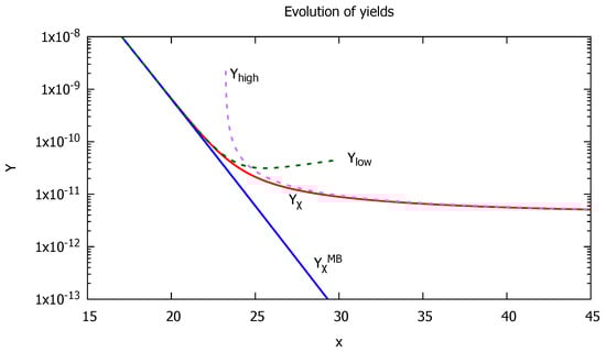
Figure 1.
Numerical plots of the evolution for each yield with parameters GeV, , , , , . The red and the blue lines show the actual evolution of and the thermal yield , respectively. The dashed lines of green and purple show the approximated solutions and , respectively.
If the interaction rate becomes much lower than the Hubble rate at the relativistic regime , the abundance freezes out with the massless abundance (hot relic):
where .
Finally, we need to mention the validity of the approximated results (72) and (74). Their behaviors can deviate easily if the master Equation (67) includes significant extra processes by other species or the singular behavior of the cross-sections. Specifically, some exceptional cases are known: (i) mutual annihilations of multiple species (coannihilations), (ii) annihilations into heaver states (forbidden channels), (iii) annihilations near a pole in the cross-section [23], and (iv) simultaneous chemical and kinetic decoupling (coscattering) [25]. In these cases, the analysis should be performed more carefully. See refs. [23,24,25,26,70,71,72] as their example cases, and also refs. [73,74,75] as examples of the evaluation with the temperature parameter. As comparisons with their results, recent papers [76,77] show results by the full Boltzmann equation without the temperature parameter.
3.2. Constraint on Relic Abundance
The relic abundance for the stable particles through the freeze-out of their annihilation processes, as similar to particles discussed above, is restricted by the cosmological observation results. A useful parameter relating to the relic abundance is the density parameter, defined by
Since the yield maintains a constant after the freeze-out unless the additional entropy production occurs in the later era, one can estimate the present density parameter of with the present values. The current observation through the the Cosmic Microwave Background [78] provides K, , km/s/Mpc, ; therefore, one can estimate
Because the present density parameter for the cold matter component is observed as and it must be larger than the component, one can obtain a bound as
The set of parameters shown in (76) is seemingly suitable for the above constraint with a bit of modification. However, that would fail by taking into account the direct detections of the DM that focuses on the process of , where is a standard model particle. If the annihilation process occurs through a similar interaction to the electroweak gauge interaction, the cross-section for - elastic scattering also relates to the same gauge interaction. One can estimate , but it is already excluded by the direct detection [79].
3.3. Relic Abundance in Freeze-In
The discussion and the result in the previous subsections are based on the freeze-out scenario in which the DM particles are in thermal equilibrium initially. However, it is not satisfied if the interaction between the DM particles and the thermal bath is too small—the so-called FIMP (feebly interacting massive particle) scenario [21,80]. In this situation, the yield of DM evolves from zero through the thermal production from the thermal bath. Although the DM never reaches the thermal equilibrium, the yield freezes in with a non-thermal yield at last.
We discuss here the relic abundance by the freeze-in scenario in two cases of the pair-creation of DM by (1) scattering from thermal scattering and (2) decay from a heavier particle.
3.3.1. Pair-Creation by Scattering
In the case that DM-pair () is produced by thermal pair particles (), the Boltzmann equation is given by (68) as
where we approximated and the adiabatic degrees until the freezing-in. For simplicity, we consider the simple interaction described by
where is the bosonic DM, labeled i are the massless bosons in the thermal bath, and y is a coupling constant. The thermally averaged cross-section is given by
where and are the degrees of freedom for each species. Therefore, one can estimate the final yield at as
This result implies that the yield freezing occurs around the earlier stage because (85) can be regarded as .
3.3.2. Pair-Creation by Decay
The other possible freeze-in scenario is due to the pair production from a heavier particle: [21,81]. The original Boltzmann equation for DM is given by
where is a decay constant and . We also approximated , , and in the second line. Therefore, the final yield can be estimated as
where is the degrees of freedom for . If the decay constant can be represented by the coupling constant y as
the required magnitude of the coupling with the relation formula to the density parameter (79) can be estimated as
4. Application to Baryogenesis
The other popular application of the Boltzmann equation in cosmology is the baryogenesis scenario that describes the dynamical evolution of the baryon number in the universe from zero at the beginning to the non-zero at present. The present abundance of the baryons can be estimated from (79). Replacing ’s mass into the nucleon mass MeV and using the present density parameter for the baryon [78], one can obtain
There are three conditions suggested by A. D. Sakharov [82] in order to develop the baryon abundance from to non-zero: (1) baryon number (B) violation, (2) C and violation, (3) non-equilibrium condition. Their brief reasons are as follows. The B violation is trivial by definition. If the baryon number violating processes conserve C or , their anti-particle processes happen with the same rate. As a result, the net baryon number is always zero. Even if the processes violate the baryon number, C and , the thermal equilibrium reduces the baryon asymmetry due to their inverse processes. The Boltzmann equation, especially, provides a powerful tool to quantify the third condition.
To see how to construct the Boltzmann equations for the baryogenesis, let us consider with a toy model, as shown in Table 1 and Table 2. The model includes Majorana-type of chiral fermions for , baryonic chiral fermions for with the common baryon number b, and a non-baryonic complex scalar . For simplicity, the baryonic fermions and the scalar are massless and they are always in the thermal equilibrium. Because are the Majorana fermion, and can be identified. Thus, once we set the fundamental interaction to provide a decay/inverse-decay processes , their anti-particle processes also exist. These 3-body interactions also induce the B-violating 2-2 scatterings exchanging fermions.

Table 1.
Matter contents and their baryon number. All the anti-particles have the opposite sign of the baryon number.
Table 2.
Possible processes up to the 4-body B-violating interactions and their variation of the baryon number. The bar () on each species denotes the anti-particle. In addition to the shown processes here, their inverse processes are also possible. Although there are elastic scatterings , , and , we omitted them because they do not change the baryon number.
We comment on the toy model introduced above. Replacing X, , into the right-handed neutrino, left-handed neutrino, Higgs doublet in the standard model, respectively, one can obtain the type-I seesaw model that can realize the well-known leptogenesis scenario [38]. However, the correspondence is incomplete: the type-I seesaw model includes the gauge interactions that induce the scattering process. See, e.g., ref. [83] for a review of the leptogenesis scenario and [60,84] for the treatment by the Kadanoff–Baym equation.
4.1. Mean Net Baryon Number
At first, we consider only the decay processes for simplicity. This situation is realized when particles start to decay after the scattering processes freeze out. Here, we define the mean net baryon number by
where the summation runs for all decay processes, and are the generated baryon number through the process of and its branching ratio, respectively. The physical meaning of the mean net baryon number is an average of the produced baryon number by a single quantum of . In the case of our toy model, this quantity can be represented as
This result reflects the requirements of B-violation and C, violation. If the decay processes are B-conserving or C, conserving processes , the mean net baryon number is vanished.
Supposing that only a single flavour survives and all of particles decay into the baryonic fermions , the generated baryon number can be estimated by . Especially, the baryon abundance can be maximized if particles are the hot relic :
where is the degrees of freedom of the Majorana-type fermion .
4.2. Boltzmann Equations in Baryogenesis Scenario
Although we considered quite a simplified situation in the previous subsection, in reality, the situation is more complicated since the system includes the dynamical decay/inverse-decay and scattering processes. In order to quantify the actual evolution of the baryon abundance including the scattering effects, we need to construct the Boltzmann equations in this system and solve them.
For simplicity, we suppose again that only a single flavor affects to the evolution of the net baryon number. Using the definition of the net baryon density , the evolution of the system including the processes in Table 2 are described by
where () is the mass (energy) of , is the total width of and
is the mean net baryon number corresponding to (95), and
is the reaction rates through the B-violating scatterings up to the tree level. (See Appendix B for the treatment of the thermally averaged quantities and, also, see Appendix C for the detail of the derivation of the equations, especially the treatment of the real intermediate state (RIS) to avoid the double-counting.) The omitted parts “…” denote the sub-leading processes in terms of the order of couplings. Equation (97) describes the dissipation of , and it converts to the baryon with the rate and flows into the baryon sector. However, the produced baryons also wash themselves out through the B-violating scattering processes due to the last term in (98). Therefore, the smaller B-violating scattering effect is favored for remaining the more net baryons as long as can be thermalized enough at the initial.
To solve the equations of motion (97) and (98), it is convenient to use the yields and the variable as
where
with the n-th order of the modified Bessel function . We assumed the adiabatic evolution of the relativistic degrees to obtain (101) and (102). The dimensionless parameters are the reaction rates normalized by the Hubble parameter. In general, is proportional to () at the limit of (), whereas the behavior of depends on the detail of the interaction, as we will see its concrete form with an example model later.
Equations (101) and (102) can provide the analytic form of as
Especially in the weakly scattering case, , one can approximate the above result as
The physical interpretation is that the whole particles existing from the beginning can convert to the net baryons without any wash-out process in this case. Hence, the approximated result does not depend on the details of the decay process . The result (107) is consistent with the former estimation in (96). On the other hand, the strongly scattering case causes a significant wash-out process, and thus, the final net baryon abundance is strongly suppressed from the result of (107).
To see the concrete evolution dynamics, we consider the following interaction
with the Yukawa coupling and the two-component spinors and . This interaction leads to the concrete representation of the decay width and the scattering rate as
where we denoted
and . Here, and are the degrees of freedom of the chiral fermion and the scalar , not including their anti-particle state. The asymptotic behaviors for each reaction rate are governed by
The actual behaviors of and with concrete parameters are shown in the upper side of Figure 2. The asymptotic behaviors at and are consistent with (114). The enhancement structures for each seen around are induced by the resonant process through the on-shell s-channel shown in (112).
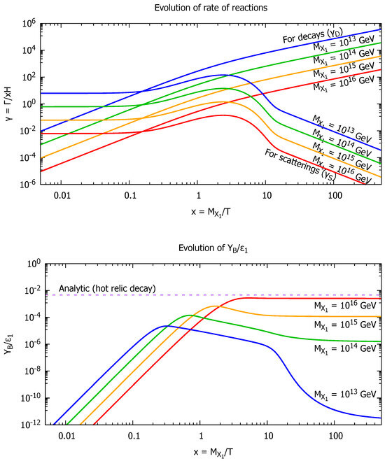
Figure 2.
Numerical plots of the evolution of the interaction rates (upper) and (lower) for each mass of X. The numerical parameters are chosen as , , , , , and assumed the thermal distribution for and at the initial point. The solid lines in red, yellow, green, and blue correspond to , and GeV, respectively. In the upper figure, “For decays” and “For scatterings” depict and , respectively. In the lower figure, the dashed line in purple shows the approximated solution (96) due to the decay of the hot relic, .
The lower side in Figure 2 shows the evolution of , which is the numerical result from the coupled Equations (101) and (102). The result shows that the heavier mass of X can generate the net baryon number more because the reaction rates are reduced for the heavier case, and hence, the generated baryons can avoid the wash-out process. Specifically, the plot for GeV leads the close result to the hot relic approximation (107), whereas the plot for GeV shows the dumping by the wash-out effect at the late stage. The milder decrease at the middle stage is caused by the decay of X particles that supply the net baryons to compensate for the wash-out effect.
Finally, the obtained yield of the net baryon number should be compared with the current bound (93), . Since the mean net baryon number can roughly be estimated by , where is a CP phase in the considered model, one can obtain the constraint from the current observation as , where we used . Therefore, one can find that GeV is allowed by comparison with the lower plot in Figure 2.
5. Summary
In this paper, we have demonstrated the derivation of the Boltzmann equation from the microscopic point of view with the quantum field theory, in which the transition probability has been constructed with the statistically averaged quantum states. Although both results of the full and the integrated Boltzmann Equations (37) and (44) are consistent with the well-known results, our derivation ensures that especially the full Boltzmann equation is widely applicable even in the non-equilibrium state, since the derivation does not assume any distribution type nor the temperature of the system. Specifically, the integrated Boltzmann Equation (44) is quite convenient and applicable to a wide range of situations. In the particular case that the kinetic equilibrium cannot be ensured, the coupled equations with the temperature parameter (58) and (59) are better for following the dynamics.
As the application examples of the (integrated) Boltzmann equation in cosmology, we have reviewed two cases: the relic abundance of the DM and the baryogenesis scenario. For the former case, we have shown the Boltzmann equation and its analysis. The analytic results (72) and (74) are quite helpful for estimating the final relic abundance of the DM and its freeze-out epoch. For the latter case, we have derived the Boltzmann equation with a specific model and shown the numerical analysis. The final net baryon number can be estimated by the analytic result (107) in the case of the weakly interacting system, whereas that is strongly suppressed by the wash-out effect in the case of the strongly interacting system.
The Boltzmann equation is a powerful tool for following the evolution of the particle number or other thermal quantities, and thus, it will be applied to many more situations in the future and will open a new frontier in current physics. We hope this paper will be helpful in using the Boltzmann equation and its techniques thoughtfully.
Author Contributions
Conceptualization, S.E. and H.-H.Z.; methodology, S.E.; validation, Y.-H.S. and M.-Z.Z.; formal analysis, S.E.; investigation, S.E.; resources, S.E.; data curation, S.E. and Y.-H.S.; writing—original draft preparation, S.E.; writing—review and editing, S.E., Y.-H.S., M.-Z.Z. and H.-H.Z.; supervision, H.-H.Z.; project administration, S.E.; funding acquisition, H.-H.Z. All authors have read and agreed to the published version of the manuscript.
Funding
This work is supported in part by the National Natural Science Foundation of China under Grant No. 12275367, and the Sun Yat-sen University Science Foundation.
Data Availability Statement
The raw data supporting the conclusions of this article will be made available by the authors on request.
Acknowledgments
We thank Chengfeng Cai, Yi-Lei Tang, and Masato Yamanaka for useful discussions and comments.
Conflicts of Interest
The authors declare no conflicts of interest. The funders had no role in the design of the study; in the collection, analyses, or interpretation of data; in the writing of the manuscript; or in the decision to publish the results.
Appendix A. Validity of the Maxwell–Boltzmann Similarity Approximation
Although the approximation of the distribution function by the Maxwell–Boltzmann similarity distribution is used well in many situations, it is not always valid. In this appendix, we show that the approximation is valid if the focusing species is in the kinetic equilibrium through interacting with the thermal bath.
Let us consider the situation of the particle number conserving process , where a and b denote the particle species. If this process happens fast enough and the species b maintains the thermal distribution, the condition of the detailed balance leads to
where we assumed the common temperature to the thermal bath and the energy conservation law: . Because the above relation must be satisfied by arbitrary energy, one can obtain
where is a function that is dependent on time but independent of the energy. The function can be determined by integrating over the momentum of , i.e., . Finally, one can obtain the desired form of the distribution:
Appendix B. Formulae for Thermal Average by Boltzmann–Maxwell Distribution
In this section, we summarize the convenient formulae used in the various thermally averaged quantities by the Maxwell–Boltzmann distribution, especially for number density, decay rate, and cross-section.
Appendix B.1. Number Density and Modified Bessel Function
The number density with the Maxwell–Boltzmann distribution is given by
where is the n-th order of the modified Bessel function given by
The following relations are helpful in analysis:
Appendix B.2. Thermally Averaged Decay Rate
The rate defined in (45) for the single initial species relates to the decay rate, , where
is the Lorentz-invariant partial width for the process . (The Lorentz invariance of the partial width is obvious because the following elements are Lorentz-invariant: , , . This argument is also applicable to show the Lorentz invariance of the cross-section.) The factor in corresponds to the inverse Lorentz gamma factor describing the life-time dilation. The thermal average of the rate is given by
Appendix B.3. Thermal Averaged Cross-Section
The rate averaged by the initial 2-species relates to the scattering rate,
where is the cross-section for the process dependent on the Mandelstam variable , and v is the Møller velocity
The thermal average of the rate can be obtained by
where the integral variable denotes the angle between and , i.e., .
In order to perform the integral in (A22), it is convenient to change the integral variables to , where [62]. The Jacobian is given by
The integral region can be obtained from the expression of the Mandelstam variable,
which leads to
The above inequality is equivalent to
Therefore, the integral region can be obtained as
where
Using the above results, the integral (A22) can be performed as
where we used the representation of the number density (A6).
Especially in the case of the non-relativistic limit, , it is convenient to use the representation
where the Lorentz-invariant “velocity” behaves as at the non-relativistic limit. Note that at remains non-zero (s-wave contribution) in general. Furthermore, the replacement of the integral variable s with y defined by
is also convenient for the calculation. Since the integral parameter y corresponds to naively, we can expect that the significant integral interval is on . Then, (A32) can be approximated as
where we used the asymptotic expansion (A9) and the Taylor series around ,
Appendix C. Derivation of the Boltzmann Equations in Baryogenesis Scenario
In this section, we demonstrate the derivation of the Boltzmann equation in the baryogenesis scenario with the processes listed in Table 2. Indeed, the straightforward derivation of the Boltzmann equations leads to the over-counting problem in the amplitudes. For example, once a contribution of the decay/inverse-decay process is included in the Boltzmann equation, the straightforward contribution from the scattering process is over-counted because such process can be divided into and if the intermediate state X is on-shell. Therefore, in general, one must regard the straightforward contribution in the scattering processes as the subtracted state of the real intermediated state (RIS) from the full contribution [9,85]:
In a case of the scattering process , the full amplitude part can be represented as
where s is the Mandelstam variable, and are X’s mass and total decay width, respectively. On the other hand, the RIS part can be evaluated as the limit of the narrow width by
In the last line, the narrow width approximation is applied. Since the contribution of both amplitudes in (A41) is the order of , the RIS contribution is also the order of in total. Therefore, the RIS part in the scattering process contributes to the decay/inverse-decay process.
Taking into account the above notice, we derive the Boltzmann equation. For simplicity, we suppose that only a single flavor affects to the evolution of the net baryon number. Because there are no scattering processes associated with , the equation governing is simply written as
where
is the total decay width of and
is the thermally averaged width, and is the modified Bessel function. To derive (A43), we assumed the universal distributions for () and ignored the chemical potentials in the thermal distributions (). Moreover, we assumed is always in the thermal equilibrium (). On the other hand, ’s equation should be derived with the consideration of the subtracted state in some scattering processes to avoid the over-counting of the decay/inverse-decay processes:
where we used the notations , , and
with are the thermally averaged cross-sections. The fourth line in (A47) corresponds to the RIS contribution that makes the thermal balance to the first line, while the processes in the third line include the resonant structure as seen in (A39). With the expression of the net baryon number density , one can finally obtain the equation for the net baryons using (A47) as
where is the mean net number defined in (99), and we used the approximation
Note that the tree level contributions of cross-sections and their anti-state are the same in general. Therefore, the terms in the second and fourth lines in (A50) are cancelled in the leading order, respectively.
References
- Alpher, R.A.; Bethe, H.; Gamow, G. The origin of chemical elements. Phys. Rev. 1948, 73, 803–804. [Google Scholar] [CrossRef]
- Hayashi, C. Proton-Neutron Concentration Ratio in the Expanding Universe at the Stages preceding the Formation of the Elements. Prog. Theor. Phys. 1950, 5, 224–235. [Google Scholar] [CrossRef]
- Alpher, R.A.; Follin, J.W.; Herman, R.C. Physical Conditions in the Initial Stages of the Expanding Universe. Phys. Rev. 1953, 92, 1347–1361. [Google Scholar] [CrossRef]
- Burbidge, G.R. Nuclear Energy Generation and Dissipation in Galaxies. Pub. Astron. Soc. Pacific 1958, 70, 83. [Google Scholar] [CrossRef]
- Hoyle, F.; Tayler, R.J. The Mystery of the Cosmic Helium Abundance. Nature 1964, 203, 1108. [Google Scholar] [CrossRef]
- Zeldovich, Y.B. Survey of Modern Cosmology. Adv. Astron. Astrophys. 1965, 3, 241–379. [Google Scholar] [CrossRef]
- Peebles, P.J.E. Primeval Helium Abundance and the Primeval Fireball. Phys. Rev. Lett. 1966, 16, 410–413. [Google Scholar] [CrossRef]
- Peebles, P.J.E. Primordial Helium Abundance and the Primordial Fireball. 2. Astrophys. J. 1966, 146, 542–552. [Google Scholar] [CrossRef]
- Kolb, E.W.; Turner, M.S. The Early Universe. Front. Phys. 1990, 69, 1–547. [Google Scholar] [CrossRef]
- Weinberg, S. Cosmology; Oxford University Press: Oxford, UK, 2008; 544p. [Google Scholar]
- Cyburt, R.H.; Fields, B.D.; Olive, K.A.; Yeh, T.H. Big Bang Nucleosynthesis: 2015. Rev. Mod. Phys. 2016, 88, 015004. [Google Scholar] [CrossRef]
- Kompaneets, A.S. The Establishment of Thermal Equilibrium between Quanta and Electrons. Zh. Eksp. Teor. Fiz. 1956, 31, 876. [Google Scholar]
- Kompaneets, A.S. The Establishment of Thermal Equilibrium between Quanta and Electrons. Sov. Phys. JETP 1957, 4, 730. [Google Scholar]
- Weymann, R. Diffusion Approximation for a Photon Gas Interacting with a Plasma via the Compton Effect. Phys. Fluids 1965, 8, 2112. [Google Scholar] [CrossRef]
- Sunyaev, R.A.; Zeldovich, Y.B. Distortions of the background radiation spectrum. Nature 1969, 223, 721. [Google Scholar] [CrossRef]
- Zeldovich, Y.B.; Sunyaev, R.A. The Interaction of Matter and Radiation in a Hot-Model Universe. Astrophys. Space Sci. 1969, 4, 301. [Google Scholar] [CrossRef]
- Sunyaev, R.; Zeldovich, Y.B. The Spectrum of Primordial Radiation, its Distortions and their Significance. Comments Astrophys. Space Phys. 1970, 2, 66. [Google Scholar]
- Sunyaev, R.; Zeldovich, Y.B. The Observations of Relic Radiation as a Test of the Nature of X-Ray Radiation from the Clusters of Galaxies. Comments Astrophys. Space Phys. 1972, 4, 173. [Google Scholar]
- Lee, B.W.; Weinberg, S. Cosmological Lower Bound on Heavy Neutrino Masses. Phys. Rev. Lett. 1977, 39, 165–168. [Google Scholar] [CrossRef]
- Scherrer, R.J.; Turner, M.S. On the Relic, Cosmic Abundance of Stable Weakly Interacting Massive Particles. Phys. Rev. D 1986, 33, 1585, Erratum in Phys. Rev. D 1986, 34, 3263. [Google Scholar] [CrossRef]
- Hall, L.J.; Jedamzik, K.; March-Russell, J.; West, S.M. Freeze-In Production of FIMP Dark Matter. J. High Energy Phys. 2010, 03, 80. [Google Scholar] [CrossRef]
- Hochberg, Y.; Kuflik, E.; Volansky, T.; Wacker, J.G. Mechanism for Thermal Relic Dark Matter of Strongly Interacting Massive Particles. Phys. Rev. Lett. 2014, 113, 171301. [Google Scholar] [CrossRef] [PubMed]
- Griest, K.; Seckel, D. Three exceptions in the calculation of relic abundances. Phys. Rev. D 1991, 43, 3191–3203. [Google Scholar] [CrossRef]
- D’Agnolo, R.T.; Ruderman, J.T. Light Dark Matter from Forbidden Channels. Phys. Rev. Lett. 2015, 115, 061301. [Google Scholar] [CrossRef] [PubMed]
- D’Agnolo, R.T.; Pappadopulo, D.; Ruderman, J.T. Fourth Exception in the Calculation of Relic Abundances. Phys. Rev. Lett. 2017, 119, 061102. [Google Scholar] [CrossRef]
- Kim, H.; Kuflik, E. Superheavy Thermal Dark Matter. Phys. Rev. Lett. 2019, 123, 191801. [Google Scholar] [CrossRef]
- Berlin, A. WIMPs with GUTs: Dark Matter Coannihilation with a Lighter Species. Phys. Rev. Lett. 2017, 119, 121801. [Google Scholar] [CrossRef] [PubMed]
- Kramer, E.D.; Kuflik, E.; Levi, N.; Outmezguine, N.J.; Ruderman, J.T. Heavy Thermal Dark Matter from a New Collision Mechanism. Phys. Rev. Lett. 2021, 126, 081802. [Google Scholar] [CrossRef]
- Garny, M.; Heisig, J.; Lülf, B.; Vogl, S. Coannihilation without chemical equilibrium. Phys. Rev. D 2017, 96, 103521. [Google Scholar] [CrossRef]
- Frumkin, R.; Hochberg, Y.; Kuflik, E.; Murayama, H. Thermal Dark Matter from Freezeout of Inverse Decays. Phys. Rev. Lett. 2023, 130, 121001. [Google Scholar] [CrossRef]
- Frumkin, R.; Kuflik, E.; Lavie, I.; Silverwater, T. Roadmap to Thermal Dark Matter Beyond the WIMP Unitarity Bound. Phys. Rev. Lett. 2023, 130, 171001. [Google Scholar] [CrossRef]
- Yoshimura, M. Unified Gauge Theories and the Baryon Number of the Universe. Phys. Rev. Lett. 1978, 41, 281–284, Erratum in Phys. Rev. Lett. 1979, 42, 746. [Google Scholar] [CrossRef]
- Toussaint, D.; Treiman, S.B.; Wilczek, F.; Zee, A. Matter-Antimatter Accounting, Thermodynamics, and Black Hole Radiation. Phys. Rev. D 1979, 19, 1036–1045. [Google Scholar] [CrossRef]
- Dimopoulos, S.; Susskind, L. On the Baryon Number of the Universe. Phys. Rev. D 1978, 18, 4500–4509. [Google Scholar] [CrossRef]
- Weinberg, S. Cosmological Production of Baryons. Phys. Rev. Lett. 1979, 42, 850–853. [Google Scholar] [CrossRef]
- Nanopoulos, D.V.; Weinberg, S. Mechanisms for Cosmological Baryon Production. Phys. Rev. D 1979, 20, 2484. [Google Scholar] [CrossRef]
- Yoshimura, M. Origin of Cosmological Baryon Asymmetry. Phys. Lett. B 1979, 88, 294–298. [Google Scholar] [CrossRef]
- Fukugita, M.; Yanagida, T. Baryogenesis without Grand Unification. Phys. Lett. B 1986, 174, 45–47. [Google Scholar] [CrossRef]
- Cohen, A.G.; Kaplan, D.B.; Nelson, A.E. Weak Scale Baryogenesis. Phys. Lett. B 1990, 245, 561–564. [Google Scholar] [CrossRef]
- Cohen, A.G.; Kaplan, D.B.; Nelson, A.E. Baryogenesis at the weak phase transition. Nucl. Phys. B 1991, 349, 727–742. [Google Scholar] [CrossRef]
- Rubakov, V.A.; Shaposhnikov, M.E. Electroweak baryon number nonconservation in the early universe and in high-energy collisions. Usp. Fiz. Nauk 1996, 166, 493–537. [Google Scholar] [CrossRef]
- Affleck, I.; Dine, M. A New Mechanism for Baryogenesis. Nucl. Phys. B 1985, 249, 361–380. [Google Scholar] [CrossRef]
- Dine, M.; Randall, L.; Thomas, S.D. Baryogenesis from flat directions of the supersymmetric standard model. Nucl. Phys. B 1996, 458, 291–326. [Google Scholar] [CrossRef]
- Akita, K.; Yamaguchi, M. A precision calculation of relic neutrino decoupling. J. Cosmol. Astropart. Phys. 2020, 2020, 12. [Google Scholar] [CrossRef]
- Kamada, K.; Yamamoto, N.; Yang, D.L. Chiral effects in astrophysics and cosmology. Prog. Part. Nucl. Phys. 2023, 129, 104016. [Google Scholar] [CrossRef]
- Ai, W.Y.; Beniwal, A.; Maggi, A.; Marsh, D.J.E. From QFT to Boltzmann: Freeze-in in the presence of oscillating condensates. J. High Energy Phys. 2024, 2, 122. [Google Scholar] [CrossRef]
- Baym, G.; Kadanoff, L.P. Conservation Laws and Correlation Functions. Phys. Rev. 1961, 124, 287–299. [Google Scholar] [CrossRef]
- Baym, G. Selfconsistent approximation in many body systems. Phys. Rev. 1962, 127, 1391–1401. [Google Scholar] [CrossRef]
- Chou, K.C.; Su, Z.B.; Hao, B.L.; Yu, L. Equilibrium and Nonequilibrium Formalisms Made Unified. Phys. Rept. 1985, 118, 1–131. [Google Scholar] [CrossRef]
- Hamaguchi, K.; Moroi, T.; Mukaida, K. Boltzmann equation for non-equilibrium particles and its application to non-thermal dark matter production. J. High Energy Phys. 2012, 1, 83. [Google Scholar] [CrossRef]
- Binder, T.; Covi, L.; Mukaida, K. Dark Matter Sommerfeld-enhanced annihilation and Bound-state decay at finite temperature. Phys. Rev. D 2018, 98, 115023. [Google Scholar] [CrossRef]
- Riotto, A. Towards a nonequilibrium quantum field theory approach to electroweak baryogenesis. Phys. Rev. D 1996, 53, 5834–5841. [Google Scholar] [CrossRef] [PubMed]
- Buchmuller, W.; Fredenhagen, S. Quantum mechanics of baryogenesis. Phys. Lett. B 2000, 483, 217–224. [Google Scholar] [CrossRef]
- Garbrecht, B.; Prokopec, T.; Schmidt, M.G. Coherent baryogenesis. Phys. Rev. Lett. 2004, 92, 061303. [Google Scholar] [CrossRef]
- Simone, A.D.; Riotto, A. Quantum Boltzmann Equations and Leptogenesis. J. Cosmol. Astropart. Phys. 2007, 8, 2. [Google Scholar] [CrossRef][Green Version]
- Cirigliano, V.; Lee, C.; Ramsey-Musolf, M.J.; Tulin, S. Flavored Quantum Boltzmann Equations. Phys. Rev. D 2010, 81, 103503. [Google Scholar] [CrossRef]
- Beneke, M.; Garbrecht, B.; Fidler, C.; Herranen, M.; Schwaller, P. Flavoured Leptogenesis in the CTP Formalism. Nucl. Phys. B 2011, 843, 177–212. [Google Scholar] [CrossRef]
- Drewes, M.; Mendizabal, S.; Weniger, C. The Boltzmann equation from quantum field theory. Phys. Lett. B 2013, 718, 1119–1124. [Google Scholar] [CrossRef]
- Berges, J. Introduction to nonequilibrium quantum field theory. AIP Conf. Proc. 2004, 739, 3–62. [Google Scholar] [CrossRef]
- Garbrecht, B. Why is there more matter than antimatter? Calculational methods for leptogenesis and electroweak baryogenesis. Prog. Part. Nucl. Phys. 2020, 110, 103727. [Google Scholar] [CrossRef]
- Srednicki, M.; Watkins, R.; Olive, K.A. Calculations of Relic Densities in the Early Universe. Nucl. Phys. B 1988, 310, 693. [Google Scholar] [CrossRef]
- Gondolo, P.; Gelmini, G. Cosmic abundances of stable particles: Improved analysis. Nucl. Phys. B 1991, 360, 145–179. [Google Scholar] [CrossRef]
- Hindmarsh, M.; Philipsen, O. WIMP dark matter and the QCD equation of state. Phys. Rev. D 2005, 71, 087302. [Google Scholar] [CrossRef]
- Drees, M.; Hajkarim, F.; Schmitz, E.R. The Effects of QCD Equation of State on the Relic Density of WIMP Dark Matter. J. Cosmol. Astropart. Phys. 2015, 6, 25. [Google Scholar] [CrossRef]
- Laine, M.; Meyer, M. Standard Model thermodynamics across the electroweak crossover. J. Cosmol. Astropart. Phys. 2015, 7, 35. [Google Scholar] [CrossRef]
- Borsanyi, S.; Fodor, Z.; Guenther, J.; Kampert, K.H.; Katz, S.D.; Kawanai, T.; Kovacs, T.G.; Mages, S.W.; Pasztor, A.; Pittler, F.; et al. Calculation of the axion mass based on high-temperature lattice quantum chromodynamics. Nature 2016, 539, 69–71. [Google Scholar] [CrossRef]
- Saikawa, K.; Shirai, S. Primordial gravitational waves, precisely: The role of thermodynamics in the Standard Model. J. Cosmol. Astropart. Phys. 2018, 5, 35. [Google Scholar] [CrossRef]
- Saikawa, K.; Shirai, S. Precise WIMP Dark Matter Abundance and Standard Model Thermodynamics. J. Cosmol. Astropart. Phys. 2020, 8, 11. [Google Scholar] [CrossRef]
- Cline, J.M.; Kainulainen, K.; Scott, P.; Weniger, C. Update on scalar singlet dark matter. Phys. Rev. D 2013, 88, 055025. [Google Scholar] [CrossRef]
- Arkani-Hamed, N.; Delgado, A.; Giudice, G.F. The Well-tempered neutralino. Nucl. Phys. B 2006, 741, 108–130. [Google Scholar] [CrossRef]
- Tulin, S.; Yu, H.B.; Zurek, K.M. Three Exceptions for Thermal Dark Matter with Enhanced Annihilation to γγ. Phys. Rev. D 2013, 87, 036011. [Google Scholar] [CrossRef]
- Ibarra, A.; Pierce, A.; Shah, N.R.; Vogl, S. Anatomy of Coannihilation with a Scalar Top Partner. Phys. Rev. D 2015, 91, 095018. [Google Scholar] [CrossRef]
- Bringmann, T.; Hofmann, S. Thermal decoupling of WIMPs from first principles. J. Cosmol. Astropart. Phys. 2007, 4, 16, Erratum in J. Cosmol. Astropart. Phys. 2016, 3, E02. [Google Scholar] [CrossRef]
- Bringmann, T. Particle Models and the Small-Scale Structure of Dark Matter. New J. Phys. 2009, 11, 105027. [Google Scholar] [CrossRef]
- Binder, T.; Bringmann, T.; Gustafsson, M.; Hryczuk, A. Early kinetic decoupling of dark matter: When the standard way of calculating the thermal relic density fails. Phys. Rev. D 2017, 96, 115010, Erratum in Phys. Rev. D 2020, 101, 099901. [Google Scholar] [CrossRef]
- Ala-Mattinen, K.; Kainulainen, K. Precision calculations of dark matter relic abundance. J. Cosmol. Astropart. Phys. 2020, 9, 40. [Google Scholar] [CrossRef]
- Ala-Mattinen, K.; Heikinheimo, M.; Kainulainen, K.; Tuominen, K. Momentum distributions of cosmic relics: Improved analysis. Phys. Rev. D 2022, 105, 12. [Google Scholar] [CrossRef]
- Aghanim, N.; Akrami, Y.; Arroja, F.; Ashdown, M.; Aumont, J.; Baccigalupi, C.; Ballardini, M.; Banday, A.J.; Barreiro, R.B.; Bartolo, N.; et al. Planck 2018 results. I. Overview and the cosmological legacy of Planck. Astron. Astrophys. 2020, 641, A1. [Google Scholar] [CrossRef]
- Roszkowski, L.; Sessolo, E.M.; Trojanowski, S. WIMP dark matter candidates and searches—Current status and future prospects. Rept. Prog. Phys. 2018, 81, 066201. [Google Scholar] [CrossRef]
- Bernal, N.; Heikinheimo, M.; Tenkanen, T.; Tuominen, K.; Vaskonen, V. The Dawn of FIMP Dark Matter: A Review of Models and Constraints. Int. J. Mod. Phys. A 2017, 32, 1730023. [Google Scholar] [CrossRef]
- Chu, X.; Hambye, T.; Tytgat, M.H.G. The Four Basic Ways of Creating Dark Matter Through a Portal. J. Cosmol. Astropart. Phys. 2012, 5, 34. [Google Scholar] [CrossRef]
- Sakharov, A.D. Violation of CP Invariance, C asymmetry, and baryon asymmetry of the universe. Pisma Zh. Eksp. Teor. Fiz. 1967, 5, 32–35. [Google Scholar] [CrossRef]
- Davidson, S.; Nardi, E.; Nir, Y. Leptogenesis. Phys. Rept. 2008, 466, 105–177. [Google Scholar] [CrossRef]
- Anisimov, A.; Buchmüller, W.; Drewes, M.; Mendizabal, S. Quantum Leptogenesis I. Annals Phys. 2011, 326, 1998–2038, Erratum in Annals Phys. 2011, 338, 376–377. [Google Scholar] [CrossRef]
- Buchmuller, W.; Bari, P.D.; Plumacher, M. Leptogenesis for pedestrians. Annals Phys. 2005, 315, 305–351. [Google Scholar] [CrossRef]


Disclaimer/Publisher’s Note: The statements, opinions and data contained in all publications are solely those of the individual author(s) and contributor(s) and not of MDPI and/or the editor(s). MDPI and/or the editor(s) disclaim responsibility for any injury to people or property resulting from any ideas, methods, instructions or products referred to in the content. |
© 2025 by the authors. Licensee MDPI, Basel, Switzerland. This article is an open access article distributed under the terms and conditions of the Creative Commons Attribution (CC BY) license (https://creativecommons.org/licenses/by/4.0/).