Mathematical Modeling of Impurity Diffusion Processes in a Multiphase Randomly Inhomogeneous Body Using Feynman Diagrams

Abstract

Modeling of impurity diffusion processes in a multiphase randomly inhomogeneous body is performed using the Feynman diagram technique. The impurity diffusion equations are formulated for each of the phases separately. Their random boundaries are subject to non-ideal contact conditions for concentration. The contact mass transfer problem is reduced to a partial differential equation describing diffusion in the body as a whole, which accounts for jump discontinuities in the searched function as well as in its derivative at the stochastic interfaces. The obtained problem is transformed into an integro-differential equation involving a random kernel, whose solution is constructed as a Neumann series. Averaging over the ensemble of phase configurations is performed. The Feynman diagram technique is developed to investigate the processes described by parabolic partial differential equations. The mass operator kernel is constructed as a sum of strongly connected diagrams. An integro-differential Dyson equation is obtained for the concentration field. In the Bourret approximation, the Dyson equation is specified for a multiphase randomly inhomogeneous medium with uniform phase distribution. The problem solution, obtained using Feynman diagrams, is compared with the solutions of diffusion problems for a homogeneous layer, one having the coefficients of the base phase and the other having the characteristics averaged over the body volume.

1. Introduction

Over the past few decades, Feynman diagrams have significantly contributed to the formulation of various theoretical predictions. They emerged as an important tool in quantum field theory calculations, but they have also contributed to the development of computational methods for many other problems of mathematical modeling of physical processes, with a special emphasis on their automation. A comprehensive overview of the present state of algorithmic Feynman diagram evaluation from a theoretical perspective is given in [1]. Two primary factors explain their high importance in modern science: an algorithmic framework developed by physicists for manipulating these diagrams and efficient algebraic programs designed to perform Feynman diagram calculations.

Feynman diagrams are a powerful research tool arising in theoretical physics over the past hundred years. Initially developed within quantum electrodynamics to compute physical process amplitudes, they have evolved into a core mathematical concept in quantum field theory. Owing to their abstract nature, they find use in areas extending beyond physical applications. A detailed analysis of Feynman diagrams and their application in scientific models as well as a description of other diagrammatic methods in mathematical physics that are used when working with series are given in [2,3,4,5]. The example of application of Feynman diagrams shows that models are understood as mathematical objects that correspond to the axioms of a certain theory and correspond to the empirical phenomenon.

Diagrammatic approaches are used as a component in the theory of analogical reasoning in mathematics, where general conditions are formulated to determine when an analogy can serve as legitimate inductive support for a mathematical hypothesis in empirical sciences [6]. The development of Feynman diagrams arose due to the ability to visualize phenomena and processes, and such visualization contributed to the formation of well-grounded mathematical modeling of many phenomena through physical interpretation [7]. Diagrammatic approaches have proven effective in computational biology and structural bioinformatics problems [8,9].

The study of the properties of Feynman diagrams has also inspired mathematicians to develop many new approaches to mathematical modeling. Utilizing response and correlation functions, the relevant Feynman diagrams were constructed and analyzed, which facilitated the formulation of a systematic perturbation theory applicable to stochastically controlled nonlinear oscillators under Gaussian white noise excitation [10].

Research on singular partial differential equations using methods of theoretical physics, in particular quantum field theory, such as Feynman diagrams, was carried out in [11]. In [12], moments of the Gaussian integral were found using the diagrammatic approach. The development of the wave functions of a harmonic oscillator using the Feynman diagram technique was found in [13]. In [14], a number of Feynman algorithmic rules enabling analytical study of large fluctuations in stochastic systems are presented, which allows for the calculation of multi-time correlation functions. Special diagram rules have been developed to simplify transformation. Mellin–Barnes representations have been used to obtain the systems of linear homogeneous differential equations corresponding to the original Feynman diagrams without the need for integration by parts [15]. The authors of [16] obtained the results of the summation of Euler series that appear in the calculations of the Feynman diagram.

The above-described methods and approaches of the Feynman diagram theory occupy a special place in the mathematical modeling of diffusion transfer processes and in convection models. When analyzing the equations and structures of solutions of a stochastic velocity field that obeys the Navier–Stokes equation describing incompressible fluid flow under the action of both regular and random external forces, the Feynman wireframe diagram method is used [17]. Using this equation, one can calculate multiple statistical properties describing the velocity field, including the variance of velocity pulsations (pair correlation function) or the average reaction of the velocity field under the influence of external forces [18]. Using the Green’s function expansion, an exact expression is presented in [19] for determining the number of distinct connected Feynman diagrams. In [20], the Green’s function expansions under perturbations at time points far from the initial state, which is formulated in terms of the Feynman diagram, are obtained. The work [21] is dedicated to theoretical modeling of heat transfer in multiphase systems exhibiting random structural inhomogeneity. The Feynman diagram technique is applied to analyze fields of temperature averaged over the ensemble of phase configurations in bodies with multiple stochastic phases. The study of averaged diffusion fields in the physical and mathematical modeling of mass transfer processes in multiphase stochastically inhomogeneous bodies using the Feynman diagram technique was carried out in [22]. A method for improving the convergence of Neumann integral series for diffusion processes has been developed. An exact reaction–diffusion equation for describing chemical reactions occurring in polymer systems was derived in [23] using diagrams similar to Feynman diagrams. It was found that, when interactions between molecules are absent, the obtained equation reduces to the classical reaction–diffusion equation, and the diagram approach can be used to obtain a more precise dynamic equation in which diffusion and reaction manifest themselves more deeply than the diffusion of small molecules.

The symmetrical properties of the diffusion process refer to the homogeneity and balance in the movement of particles from areas of high concentration to areas of low concentration. In a symmetric diffusion process, particles are distributed uniformly in all directions, resulting in a homogeneous distribution over time. Key aspects of symmetry in diffusion include diffusion isotropy. This occurs when the speed of diffusion is the same in all directions and the medium within which the particles diffuse has no impact on the speed, resulting in a symmetrical distribution. Mathematical models of diffusion based on Fick’s laws assume symmetry to simplify the calculations, and the corresponding solutions to the parabolic equations reflect homogeneous concentration changes in space and time. In practical scenarios, symmetry may be affected by boundaries or constraints. For example, in a closed medium, diffusion can be symmetric until it reaches the walls, and after that point in time, the symmetry can be broken due to reflection or absorption. Thus, symmetry in diffusion is an important concept that helps to analyze and predict the behavior of particles as they move and propagate in different media.

Symmetry in diffusion and Feynman diagrams can be understood through various contexts in physics. Many physical theories demonstrate symmetries that are represented in Feynman diagrams. The results of this article can be used to analyze how diffusion processes and the Feynman diagrams used to visualize them reflect the fundamental symmetries that govern the behavior of systems in physics and to analyze the symmetry of Green’s functions, being an important aspect in the context of field theory.

The analysis of applying diagrammatic approaches to the mathematical modeling of processes of a probabilistic nature shows the effectiveness (in particular, computational) of such methods. Therefore, the purpose of the research conducted in this paper is to apply the Feynman diagram technique to the mathematical modeling of impurity diffusion processes in a multiphase body with random inhomogeneities. To achieve this aim, we follow the steps below:

• The problems for the impurity diffusion are formulated for each phase separately and include non-ideal conditions for the concentration function at random phase contact boundaries.
• The contact mass transfer problem, which takes into consideration the jumps of the searched function and its derivative at stochastic interphases, is reduced to a parabolic partial differential equation for the entire body domain.
• The obtained problem is reduced to an integro-differential equation with a random kernel.
• The Feynman diagram technique is developed to study the mass transfer processes described by such parabolic equations.
• The solution of the problem is constructed using Feynman diagrams.
• The Dyson equation is obtained in graphical and analytical forms.
• The resulting solution under uniform distribution of the phases is compared with solutions of mass transfer problems in a homogeneous layer with base phase coefficients and in a homogeneous layer with characteristics averaged over the body volume.

2. Formulation of the Contact Initial-Boundary Value Problem of Diffusion in a Multiphase Stochastically Inhomogeneous Body

Let us consider the diffusion of an impurity in a multiphase randomly inhomogeneous body, which consists of $N+1$ solid phases that are different in density and have different diffusion coefficients, a matrix, and inclusions of arbitrary shape (Figure 1). At the same time, the precise spatial configuration of the phases within the body region is unknown. Then, the disposition of the inclusions is not known, but we assume that the law of their probability distribution is known [24]. Furthermore, suppose that the matrix volume fraction significantly exceeds that of the inclusion, $v_j<<v_0$ ($j=1,\dots ,N$). The assumption is made that the material density and diffusion coefficient are constant in each of the phases.

Note that it is possible that two inclusions, when in contact with each other, touch along a line (curve) or at a point. Then, the total area (length) of such inclusion contacts is $\left|{\displaystyle \sum _{\begin{array}{l}\mathrm{all}\hspace{0.17em}\mathrm{contact}\\ \mathrm{points}\end{array}}{\Gamma }_{ji}}\right|=mes\hspace{0.17em}0$, and this quantity can be neglected.

To determine concentrations $c_j\left(\overrightarrow{r},t\right)$ of the impurity in the matrix (region $(V_0)$) and the inclusions (regions $(V_j)$, $j=1,\dots ,N$) at the absence of internal mass sources, the diffusion equations [25,26] formulated for each phase separately are used:

$${\rho }_j{\displaystyle \frac{\partial c_j\left(\overrightarrow{r},t\right)}{\partial t}}=d_j\Delta c_j\left(\overrightarrow{r},t\right), \overrightarrow{r}\in (V_j), t\in \left[0,\tau \right],\hspace{0.17em}\tau <\infty .$$

(1)

Here, ${\rho }_j$ is the density of the matter in the random region $(V_j)$; $d_j={\rho }_j{D}_j$ is the kinetic coefficient of impurity transfer to $(V_j)$; $D_j$ is the diffusion coefficient; $\overrightarrow{r}=(x,y,z)$ is the radius vector of a moving point; and t denotes time.

Suppose that the inclusions are located exclusively in the body region, that is, the matrix is located on the outer boundary of the body. Initial and boundary conditions are prescribed as follows:

$${\left.c_j(\overrightarrow{r},t)\right|}_{t=0}={\widehat{c}}_j(\overrightarrow{r}) (j=0,\dots ,N),\hspace{1em}{\left.c_0(\overrightarrow{r},t)\right|}_{\overrightarrow{r}\in \delta V}=\tilde{c}(t).$$

(2)

In otherwords, the initial distribution of the impurity concentration field is known, and the concentration values on the body’s boundary are maintained.

At the interfaces, e.g., the boundaries between the regions $(V_0)$ and $(V_j)$($j=1,\dots ,N$), the conditions of non-ideal mass contact with respect to concentration are imposed [27,28]:

$${\left.k_j{c}_j(\overrightarrow{r},t)\hspace{0.17em}\right|}_{\hspace{0.17em}\overrightarrow{r}\in {\Gamma }_{jl}-0}={\left.k_l{c}_l(\overrightarrow{r},t)\hspace{0.17em}\right|}_{\hspace{0.17em}\overrightarrow{r}\in {\Gamma }_{jl}+0};$$

(3)

$${\left.{\rho }_j{d}_j\overrightarrow{\nabla }{c}_j(\overrightarrow{r},t)\right|}_{\hspace{0.17em}\overrightarrow{r}\in \Gamma jl-0}={\left.{\rho }_l{d}_l\overrightarrow{\nabla }{c}_l(\overrightarrow{r},t)\right|}_{\hspace{0.17em}\overrightarrow{r}\in {\Gamma }_{jl}+0}, j,l=1,\dots ,N,$$

(4)

where $k_{s\hspace{0.17em}}$$(s=j,l)$ is the coefficient describing the concentrationdependence of the particles’ chemical potential in phase $s$ [27], which determines the magnitude of the concentration-field jump at the interfacial boundaries, and ${\Gamma }_{ji}$ is the boundary of the ith simply connected region of the jth phase $(V_{ji})$. Moreover,

$$\Gamma ={\displaystyle \underset{j=0}{\overset{N}{\cup }}{\displaystyle \underset{i=1}{\overset{n_j}{\cup }}{\Gamma }_{ji}}},$$

(5)

is the total phase contact boundary, and $n_j$ is the number of simply connected regions in the phase $j$. In this problem’s statement, the random quantities are the contact surfaces, i.e., the boundaries of the regions $(V_{ji})$, which are internal for the body, which leads to stochasticity of the concentration field of the diffusing matter.

3. Equation of Mass Transfer for the Entire Body

Let us reduce the contact problem of diffusion (1), (3), and (4) to the mass transfer equation for a body in general. For this purpose, let us define a random function of the spatial coordinate $c(\overrightarrow{r},t)$ that characterizes concentration field in the body as a whole:

$$c(\overrightarrow{r},t)=\left\{\begin{array}{l}{c}_j(\overrightarrow{r},t),\hspace{0.17em}\hspace{0.17em}\hspace{0.17em}\hspace{0.17em}\hspace{0.17em}\overrightarrow{r}\in (V_j),\hspace{0.17em}\hspace{1em}j=0,\dots ,N;\\ contact\hspace{0.17em}\hspace{0.33em}conditions \hspace{0.33em}\left(3\right),\hspace{0.17em}\hspace{0.17em}\left(4\right),\hspace{0.17em}\hspace{0.33em}\hspace{0.17em}\overrightarrow{r}\in \Gamma . \end{array}\right.\hspace{0.17em}\hspace{0.17em}$$

(6)

Let us seek $\overrightarrow{\nabla }c(\overrightarrow{r},t)$, considering that the concentration field $c(\overrightarrow{r},t)$ has first kind jump discontinuities (conditions (3), (4)) on the boundaries of contact between regions $\Gamma$. Therefore, we obtain [29]

$$\overrightarrow{\nabla }c(\overrightarrow{r},t)=\left\{\overrightarrow{\nabla }c(\overrightarrow{r},t)\right\}+{[c(\overrightarrow{r},t)]}_{\Gamma }\delta (\overrightarrow{r}-{\overrightarrow{r}}_{\Gamma }),$$

(7)

where ${\overrightarrow{r}}_{\Gamma }$ is the radius vector of the boundary $\Gamma$ points; $\left\{\dots \right\}$ are the regions of continuity of the function; ${[\dots ]}_{\Gamma }$ is the function jump at the boundary $\Gamma$; and $\delta (\cdot )$ stands for the delta function.

We observe that the jump ${[c(\overrightarrow{r},t)]}_{\Gamma }=$$({\left.c(\overrightarrow{r},t)\right|}_{{\Gamma }_{-}}\cdot {\overrightarrow{n}}_{\Gamma })+{\left.(c(\overrightarrow{r},t)\right|}_{{\Gamma }_{+}}\cdot {\overrightarrow{n}}_{\Gamma })$ (${\overrightarrow{n}}_{\Gamma }$) is unit normal vector to the contact boundary) is in fact a vector quantity and varies with the radius vector $\overrightarrow{r}\in \Gamma$.

The quantity $\Delta c(\overrightarrow{r},t)$ is found in the same way as (7), considering that the function $\overrightarrow{\nabla }c(\overrightarrow{r},t)$ has first kind jump discontinuities on the surfaces of phase division (conditions (4)). Then, we have

$$\Delta c(\overrightarrow{r},t)=\left\{\Delta c(\overrightarrow{r},t)\right\}+{\left[\overrightarrow{\nabla }c(\overrightarrow{r},t)\right]}_{\Gamma }\delta (\overrightarrow{r}-{\overrightarrow{r}}_{\Gamma })+{[c(\overrightarrow{r},t)]}_{\Gamma }\cdot \overrightarrow{\nabla }\delta (\overrightarrow{r}-{\overrightarrow{r}}_{\Gamma }).$$

(8)

Coefficients $d(\overrightarrow{r})$ and $\rho (\overrightarrow{r})$ are designated for open regions, namely

$$d(\overrightarrow{r})={\displaystyle \sum _{j=0}^N{\left\{d_j\right\}}_{\overrightarrow{r}\in (V_j)\backslash \Gamma }} \mathrm{and} \rho (\overrightarrow{r})={\displaystyle \sum _{j=0}^{\mathrm{N}}{\left\{{\rho }_j\right\}}_{\overrightarrow{r}\in (V_j)\backslash \Gamma }}.$$

(9)

At the same time, at the contact boundaries of $\overrightarrow{r}\in \Gamma$, a jump of these coefficients takes place ${\left[\rho (\overrightarrow{r})\right]}_{\overrightarrow{r}\in {\Gamma }_{ji}}$, ${\left[d(\overrightarrow{r})\right]}_{\overrightarrow{r}\in {\Gamma }_{ji}}$.

Note that the relation for the stochastic field of impurity concentration in the whole body (6) completely describes the function $c\left(\overrightarrow{r},t\right)$ for $\overrightarrow{r}\in (V)$, $t\in \left[0,\tau \right]$.

Let us introduce the random operator ${\eta }_{ij}(\overrightarrow{r})$ as the “structure function”, which is defined as follows:

$${\eta }_{ji}\left(\overrightarrow{r}\right)=\left\{\begin{array}{l}1,\hspace{0.17em}\hspace{0.33em}if\hspace{0.17em}\hspace{0.17em}\overrightarrow{r}\in (V_{ji}),\\ 0,\hspace{0.33em}\hspace{0.17em}if\hspace{0.17em}\hspace{0.17em}\overrightarrow{r}\notin (V_{ji}),\end{array}\right.$$

(10)

which satisfies the condition of body solidity

$${\displaystyle \sum _{j=0}^N\hspace{0.17em}{\displaystyle \sum _{i=1}^{n_j}\hspace{0.17em}{\eta }_{ji}(\overrightarrow{r})}}=1.$$

(11)

Note that the probability law of the structural function ${\eta }_{ij}(\overrightarrow{r})$ matches the given probability law for the distribution of phases in the body.

Then, the kinetic coefficient $d(\overrightarrow{r})$ and the density $\rho (\overrightarrow{r})$ can be represented using a random structure function (10) as follows:

$$\rho (\overrightarrow{r})={\displaystyle \sum _{j=0}^N{\displaystyle \sum _{i=1}^{n_j}{\rho }_j{\eta }_{ji}(\overrightarrow{r})}}, d(\overrightarrow{r})={\displaystyle \sum _{j=0}^N{\displaystyle \sum _{i=1}^{n_j}{d}_j{\eta }_{ji}(\overrightarrow{r})}}.$$

(12)

For the body as a whole, the mass balance equation holds

$$\rho \left(\overrightarrow{r}\right){\displaystyle \frac{\partial c\left(\overrightarrow{r},t\right)}{\partial t}}=-\overrightarrow{\nabla }\cdot \overrightarrow{J}\left(\overrightarrow{r},t\right),$$

(13)

Here, $\overrightarrow{J}\left(\overrightarrow{r},t\right)=d\left(\overrightarrow{r}\right)\overrightarrow{\nabla }c\left(\overrightarrow{r},t\right)$ is the impurity flow.

Let us take into consideration that $d(\overrightarrow{r})$ is a piecewise-constant function and has first kind jump discontinuities at the contact surfaces; then, the action of the nabla operator on it leads to

$$\overrightarrow{\nabla }d(\overrightarrow{r})={\left\{\overrightarrow{\nabla }d(\overrightarrow{r})\right\}}_{\overrightarrow{r}\in (V_{ji})}+{\left[d(\overrightarrow{r})\right]}_{\overrightarrow{r}\in \Gamma }\delta (\overrightarrow{r}-{\overrightarrow{r}}_{\Gamma }).$$

(14)

Since we assumed the problem coefficients to be constant in each phase, Formula (14) reduces to the form

$$\overrightarrow{\nabla }d(\overrightarrow{r})={\left[d(\overrightarrow{r})\right]}_{\overrightarrow{r}\in \Gamma }\delta (\overrightarrow{r}-{\overrightarrow{r}}_{\Gamma }).$$

(15)

Taking into account the ratios (7), (8), and (15), we present the Equation (13) as follows:

$$\begin{gathered} \rho (\overrightarrow{r}){\displaystyle \frac{\partial c(\overrightarrow{r},t)}{\partial t}}=\left\{d(\overrightarrow{r})\right\}\left\{\Delta c(\overrightarrow{r},t)\right\}+{\left[d(\overrightarrow{r})\right]}_{\Gamma }{\left[\overrightarrow{\nabla }c(\overrightarrow{r},t)\right]}_{\Gamma }\delta (\overrightarrow{r}-{\overrightarrow{r}}_{\Gamma }) \\ +{\left[d(\overrightarrow{r})\right]}_{\Gamma }{\left[c(\overrightarrow{r},t)\right]}_{\Gamma }\overrightarrow{\nabla }\delta (\overrightarrow{r}-{\overrightarrow{r}}_{\Gamma })+{\left[d(\overrightarrow{r})\right]}_{\Gamma }{\left[c(\overrightarrow{r},t)\right]}_{\Gamma }{\delta }^2(\overrightarrow{r}-{\overrightarrow{r}}_{\Gamma }). \end{gathered}$$

(16)

It is taken into consideration here that the function $c(\overrightarrow{r},t)$ is a piecewise continuous one in time together with the first derivative. It is also accepted that the regions of continuity of the kinetic coefficient $d(\overrightarrow{r})$ and the function $c(\overrightarrow{r},t)$ coincide:$\left\{d(\overrightarrow{r})\right\}\left\{c(\overrightarrow{r},t)\right\}=\left\{d(\overrightarrow{r})c(\overrightarrow{r},t)\right\}$.

Using the condition of body solidity (11) and representations (12), the equation for the entire body is written as

$$\begin{gathered} L(\overrightarrow{r},t)c(\overrightarrow{r},t)\equiv {\displaystyle \sum _{j=0}^N{\displaystyle \sum _{i=1}^{n_j}{\rho }_j{\eta }_{ji}}}(\overrightarrow{r}){\displaystyle \frac{\partial c}{\partial t}}-{\displaystyle \sum _{j=0}^N{\displaystyle \sum _{i=1}^{n_j}{d}_j}}{\eta }_{ji}(\overrightarrow{r})\Delta c(\overrightarrow{r},t) \\ -{\displaystyle \frac{1}{2}}{\displaystyle \sum _{j=0}^N{\displaystyle \sum _{i=1}^{n_j}{\left[d(\overrightarrow{r})\right]}_{{\Gamma }_{ji}}{\left[\overrightarrow{\nabla }c(\overrightarrow{r},t)\right]}_{{\Gamma }_{ji}}}}\delta (\overrightarrow{r}-{\overrightarrow{r}}_{{\Gamma }_{ji}})-{\displaystyle \frac{1}{2}}{\displaystyle \sum _{j=0}^N{\displaystyle \sum _{i=1}^{n_j}{\left[d(\overrightarrow{r})\right]}_{{\Gamma }_{ji}}{\left[\overrightarrow{\nabla }c(\overrightarrow{r},t)\right]}_{{\Gamma }_{ji}}}}\overrightarrow{\nabla }\delta (\overrightarrow{r}-{\overrightarrow{r}}_{{\Gamma }_{ji}}) \\ -{\displaystyle \frac{1}{2}}{\displaystyle \sum _{j=0}^N{\displaystyle \sum _{i=1}^{n_j}{\left[d(\overrightarrow{r})\right]}_{{\Gamma }_{ji}}{\left[c(\overrightarrow{r},t)\right]}_{{\Gamma }_{ji}}}}{\delta }^2(\overrightarrow{r}-{\overrightarrow{r}}_{{\Gamma }_{ji}})=0. \end{gathered}$$

(17)

In Equation (17), let us add and subtract the deterministic operator $L_0(\overrightarrow{r},t)$ with coefficients that are characteristics of the base phase (matrix)

$$L_0(\overrightarrow{r},t)=\hspace{0.17em}{\rho }_0{\displaystyle \frac{\partial }{\partial t}}-d_0\Delta .$$

Then, we will obtain

$$L_0(\overrightarrow{r},t)c(\overrightarrow{r},t)=L_s(\overrightarrow{r},t)c(\overrightarrow{r},t),$$

(18)

Here, $L_s(\overrightarrow{r},t)$ is the following:

$$L_s(\overrightarrow{r},t)={\displaystyle \sum _{j=1}^N({\rho }_0-{\rho }_j)}{\displaystyle \sum _{i=1}^{n_j}{\eta }_{ji}(\overrightarrow{r})\frac{\partial }{\partial t}}-{\displaystyle \sum _{j=1}^N(d_0-d_j)}{\displaystyle \sum _{i=1}^{n_j}{\eta }_{ji}(\overrightarrow{r})\Delta }$$

$$+{\displaystyle \frac{1}{2}}{\displaystyle \sum _{j=0}^N{\displaystyle \sum _{i=1}^{n_j}{\left[d(\overrightarrow{r})\right]}_{{\Gamma }_{ji}}{\left[\overrightarrow{\nabla }\dots \right]}_{{\Gamma }_{ji}}}}\delta \left(\overrightarrow{r}-{\overrightarrow{r}}_{{\Gamma }_{ji}}\right)+{\displaystyle \frac{1}{2}}{\displaystyle \sum _{j=0}^N{\displaystyle \sum _{i=1}^{n_j}{\left[d(\overrightarrow{r})\right]}_{{\Gamma }_{ji}}{\left[\dots \right]}_{{\Gamma }_{ji}}}}\overrightarrow{\nabla }\delta \left(\overrightarrow{r}-{\overrightarrow{r}}_{{\Gamma }_{ji}}\right)$$

$$+{\displaystyle \frac{1}{2}}{\displaystyle \sum _{j=0}^N{\displaystyle \sum _{i=1}^{n_j}{\left[d(\overrightarrow{r})\right]}_{{\Gamma }_{ji}}{\left[\dots \right]}_{{\Gamma }_{ji}}}}{\delta }^2\left(\overrightarrow{r}-{\overrightarrow{r}}_{{\Gamma }_{ji}}\right).$$

(19)

Thus, a stochastic differential equation of the mass transfer of an impurity for a medium with randomly located inclusions was obtained in the form of (17), and a “perturbed” differential equation was obtained in the form of (18) with a random operator (19).

4. Integro-Differential Mass Transfer Equation:Neumann Series

Treating the right-hand side of Expression (18) as a source for the mass transfer process in a stochastically non-homogeneous multiphase body, we construct an integro-differential equation that is the equivalent of the contact-boundary problems (1)–(4) considered initially [27]:

$$c(\overrightarrow{r},t)=c_h(\overrightarrow{r},t)+{\displaystyle \underset{0}{\overset{t}{\int }}{\displaystyle \underset{(V)}{\int }G(\overrightarrow{r},{\overrightarrow{r}}^{\prime },t,t^{\prime })L_s({\overrightarrow{r}}^{\prime },t^{\prime })c({\overrightarrow{r}}^{\prime },t^{\prime })}\hspace{0.17em}d{\overrightarrow{r}}^{\prime }d{t}^{\prime }}.$$

(20)

with $c_h(\overrightarrow{r},t)$ representing the solution of the homogeneous initial boundary value problem

$$L_0(\overrightarrow{r},t)c_h(\overrightarrow{r},t)=0,$$

(21)

$${\left.c_h(\overrightarrow{r},t)\right|}_{\overrightarrow{r}\in \delta V}=\tilde{c}(t), {\left.c_h(\overrightarrow{r},t)\right|}_{t=0}={\widehat{c}}_0(\overrightarrow{r});$$

(22)

$G(\overrightarrow{r},{\stackrel{{\displaystyle \rightharpoonup }}{r}}^{\prime },t,t^{\prime })$ is the Green’s function, which is obtained as the solution to a deterministic initial boundary value problem that includes a point source

$$L_0(\overrightarrow{r},t)G(\overrightarrow{r},{\overrightarrow{r}}^{\prime },t,t^{\prime })=\delta (t-t^{\prime })\delta (\overrightarrow{r}-{\overrightarrow{r}}^{\prime }),$$

(23)

$${\left.G(\overrightarrow{r},{\overrightarrow{r}}^{\prime },t,t^{\prime })\right|}_{\overrightarrow{r}\in \delta V}=0, {\left.G(\overrightarrow{r},{\overrightarrow{r}}^{\prime },t,t^{\prime })\right|}_{t=0}=0.$$

(24)

The solution of the integro-differential Equation (20) is constructed as a Neumann integral series expansion. This equation is satisfied for all the points $(\overrightarrow{r},t)$ in the field of definition, in particular at the point $({\overrightarrow{r}}^{\prime },t^{\prime })$. Let us write an expression for the concentration field $c(\overrightarrow{r},t)$ at the point $({\overrightarrow{r}}^{\prime },t^{\prime })$,

$$c({\overrightarrow{r}}^{\prime },t^{\prime })=c_h({\overrightarrow{r}}^{\prime },t^{\prime })+{\displaystyle \underset{0}{\overset{t^{\prime }}{\int }}{\displaystyle \underset{(V)}{\int }G({\overrightarrow{r}}^{\prime },{\overrightarrow{r}}^{″},t^{\prime },t^{″})L_s({\overrightarrow{r}}^{″},t^{″})c({\overrightarrow{r}}^{″},t^{″})}\hspace{0.17em}\hspace{0.17em}\hspace{0.17em}d{\overrightarrow{r}}^{″}d{t}^{″}},$$

(25)

and substitute the obtained relation (25) into the integro-differential Equation (20):

$$c(\overrightarrow{r},t)=c_h(\overrightarrow{r},t)+{\displaystyle \underset{0}{\overset{t}{\int }}{\displaystyle \underset{(V)}{\int }G(\overrightarrow{r},{\overrightarrow{r}}^{\prime },t,t^{\prime })L_s({\overrightarrow{r}}^{\prime },t^{\prime })}{c}_h({\overrightarrow{r}}^{\prime },t^{\prime })\hspace{0.17em}\hspace{0.17em}\hspace{0.17em}d{\overrightarrow{r}}^{\prime }d{t}^{\prime }}$$

$$+{\displaystyle \underset{0}{\overset{t}{\int }}{\displaystyle \underset{(V)}{\int }G(\overrightarrow{r},{\overrightarrow{r}}^{\prime },t,t^{\prime })L_s({\overrightarrow{r}}^{\prime },t^{\prime })}{\displaystyle \underset{0}{\overset{t^{\prime }}{\int }}{\displaystyle \underset{(V)}{\int }G({\overrightarrow{r}}^{\prime },{\overrightarrow{r}}^{″},t^{\prime },t^{″})L_s({\overrightarrow{r}}^{″},t^{″})}c({\overrightarrow{r}}^{″},t^{″})\hspace{0.17em}\hspace{0.17em}\hspace{0.17em}d{\overrightarrow{r}}^{″}d{t}^{″}}d{\overrightarrow{r}}^{\prime }d{t}^{\prime }}.$$

(26)

Equation (20) is true for all the points $(\overrightarrow{r},t)$ in the field of definition, in particular at the point $({\overrightarrow{r}}^{″},t^{″})$.

$$c({\overrightarrow{r}}^{″},t^{″})=c_h({\overrightarrow{r}}^{″},t^{″})+{\displaystyle \underset{0}{\overset{t^{″}}{\int }}{\displaystyle \underset{(V)}{\int }G({\overrightarrow{r}}^{″},{\overrightarrow{r}}^{‴},t^{″},t^{‴})L_s({\overrightarrow{r}}^{‴},t^{‴})}c({\overrightarrow{r}}^{‴},t^{‴})\hspace{0.17em}\hspace{0.17em}\hspace{0.17em}d{\overrightarrow{r}}^{‴}d{t}^{‴}}.$$

(27)

Let us substitute (27) in (26). We obtain

$$c(\overrightarrow{r},t)=c_h(\overrightarrow{r},t)+{\displaystyle \underset{0}{\overset{t}{\int }}{\displaystyle \underset{(V)}{\int }G(\overrightarrow{r},{\overrightarrow{r}}^{\prime },t,t^{\prime })L_s({\overrightarrow{r}}^{\prime },t^{\prime })}{c}_h({\overrightarrow{r}}^{\prime },t^{\prime })\hspace{0.17em}\hspace{0.17em}\hspace{0.17em}d{\overrightarrow{r}}^{\prime }d{t}^{\prime }}$$

$$+{\displaystyle \underset{0}{\overset{t}{\int }}{\displaystyle \underset{(V)}{\int }G(\overrightarrow{r},{\overrightarrow{r}}^{\prime },t,t^{\prime })L_s({\overrightarrow{r}}^{\prime },t^{\prime })}{\displaystyle \underset{0}{\overset{t^{\prime }}{\int }}{\displaystyle \underset{(V)}{\int }G({\overrightarrow{r}}^{\prime },{\overrightarrow{r}}^{″},t^{\prime },t^{″})L_s({\overrightarrow{r}}^{″},t^{″})}{c}_h({\overrightarrow{r}}^{″},t^{″})\hspace{0.17em}\hspace{0.17em}\hspace{0.17em}d{\overrightarrow{r}}^{″}d{t}^{″}}d{\overrightarrow{r}}^{\prime }d{t}^{\prime }}$$

$$+{\displaystyle \underset{0}{\overset{t}{\int }}{\displaystyle \underset{(V)}{\int }G(\overrightarrow{r},{\overrightarrow{r}}^{\prime },t,t^{\prime })L_s({\overrightarrow{r}}^{\prime },t^{\prime })}{\displaystyle \underset{0}{\overset{t^{\prime }}{\int }}{\displaystyle \underset{(V)}{\int }G({\overrightarrow{r}}^{\prime },{\overrightarrow{r}}^{″},t^{\prime },t^{″})L_s({\overrightarrow{r}}^{″},t^{″})}\hspace{0.17em}\hspace{0.17em}\hspace{0.17em}}}$$

$$\times {\displaystyle \underset{0}{\overset{t^{″}}{\int }}{\displaystyle \underset{(V)}{\int }G({\overrightarrow{r}}^{″},{\overrightarrow{r}}^{‴},t^{″},t^{‴})L_s({\overrightarrow{r}}^{‴},t^{‴})}c({\overrightarrow{r}}^{‴},t^{‴})d{\overrightarrow{r}}^{‴}d{t}^{‴}}d{\overrightarrow{r}}^{″}d{t}^{″}d{\overrightarrow{r}}^{\prime }d{t}^{\prime }.$$

(28)

As a result of an infinite iterative process, the Neumann series is obtained, namely

$$c(\overrightarrow{r},t)=c_h(\overrightarrow{r},t)+{\displaystyle \underset{0}{\overset{t}{\int }}{\displaystyle \underset{(V)}{\int }G(\overrightarrow{r},{\overrightarrow{r}}^{\prime },t,t^{\prime })L_s({\overrightarrow{r}}^{\prime },t^{\prime })}{c}_h({\overrightarrow{r}}^{\prime },t^{\prime })\hspace{0.17em}\hspace{0.17em}\hspace{0.17em}d{\overrightarrow{r}}^{\prime }d{t}^{\prime }}$$

$$+{\displaystyle \underset{0}{\overset{t}{\int }}{\displaystyle \underset{(V)}{\int }G(\overrightarrow{r},{\overrightarrow{r}}^{\prime },t,t^{\prime })L_s({\overrightarrow{r}}^{\prime },t^{\prime })}{\displaystyle \underset{0}{\overset{t^{\prime }}{\int }}{\displaystyle \underset{(V)}{\int }G({\overrightarrow{r}}^{\prime },{\overrightarrow{r}}^{″},t^{\prime },t^{″})L_s({\overrightarrow{r}}^{″},t^{″})}{c}_h({\overrightarrow{r}}^{″},t^{″})\hspace{0.17em}\hspace{0.17em}\hspace{0.17em}d{\overrightarrow{r}}^{″}d{t}^{″}}d{\overrightarrow{r}}^{\prime }d{t}^{\prime }}$$

$$+{\displaystyle \underset{0}{\overset{t}{\int }}{\displaystyle \underset{(V)}{\int }G(\overrightarrow{r},{\overrightarrow{r}}^{\prime },t,t^{\prime })L_s({\overrightarrow{r}}^{\prime },t^{\prime })}{\displaystyle \underset{0}{\overset{t^{\prime }}{\int }}{\displaystyle \underset{(V)}{\int }G({\overrightarrow{r}}^{\prime },{\overrightarrow{r}}^{″},t^{\prime },t^{″})L_s({\overrightarrow{r}}^{″},t^{″})}}}$$

$$\times {\displaystyle \underset{0}{\overset{t^{″}}{\int }}{\displaystyle \underset{(V)}{\int }G({\overrightarrow{r}}^{″},{\overrightarrow{r}}^{‴},t^{″},t^{‴})L_s({\overrightarrow{r}}^{‴},t^{‴})}{c}_h({\overrightarrow{r}}^{‴},t^{‴})d{\overrightarrow{r}}^{‴}d{t}^{‴}}d{\overrightarrow{r}}^{″}d{t}^{″}d{\overrightarrow{r}}^{\prime }d{t}^{\prime }+\dots .$$

(29)

Proposition 1.

If the densities ${\rho }_0$, ${\rho }_j$($j=1,\dots ,N$) and the diffusion coefficients $d_0$, $d_j$($j=1,\dots ,N$) are bounded and ${\rho }_0\ne 0$, $d_0\ne 0$, the for bounded $V$Neumann integral series (29) is absolutely and uniformly convergent.

The proof of this Proposition is given in Appendix A.

Moreover, the convergence of the Neumann series (29) does not depend on the values of the coefficients $k_j$ ($j=0,\dots ,N$), which determine the magnitude of the jump of the concentration function at the random interfacial boundaries. The proof also does not invoke any condition on the existence of characteristic inclusion sizes. However, one must know (as an input parameter of the problem) the number of inclusions $n_j$ ($j=0,\dots ,N$) or, at least, that the number of inclusions in the body is finite and, for example, does not exceed $N_j$: $n_j\le N_j<\infty$.

We also note that, for $t\to \infty$, in the stationary case, the Neumann series is divergent under sufficiently weak constraints since, in the stationary case, the domain of convergence of the series is significantly smaller than in the non-stationary case [30].

Since $c_h(\overrightarrow{r},t)$ is a continuously differentiable function, then the jump discontinuities of the function and its derivative across the boundary are equal to 0. Then,

$$L_s(\overrightarrow{r},t)c_h(\overrightarrow{r},t)={\displaystyle \sum _{j=1}^N({\rho }_0-{\rho }_j)}{\displaystyle \sum _{i=1}^{n_j}{\eta }_{ji}(\overrightarrow{r})\frac{\partial c_h(\overrightarrow{r},t)}{\partial t}}$$

$$-{\displaystyle \sum _{j=1}^N(d_0-d_j)}{\displaystyle \sum _{i=1}^{n_j}{\eta }_{ji}(\overrightarrow{r})\Delta }{c}_h(\overrightarrow{r},t).$$

(30)

The initial term of the Neumann series corresponds to the function $c_h(\overrightarrow{r},t)$ in a homogeneous body having the properties of the base phase. The second term represents the sum of the concentration field perturbations that arise when inclusions are inserted into the body one by one, the third one describes the pairwise influence of the inclusions on the concentration field, etc. In this case, the effects of jumps in the diffusion coefficient at the interphase boundaries are taken into account, which is ensured by the operator $L_s$.

5. Feynman Diagram Technique for Mass Transfer Problems in a Stochastically Inhomogeneous Medium

The Neumann series (29) expresses the random concentration field as a series of perturbations resulting from inclusions with diffusion characteristics distinct from those of the matrix. To examine the structure of this series, a diagrammatic representation of its terms based on R. Feynman diagrams [31] is introduced. Here, the typical notations are used [32].

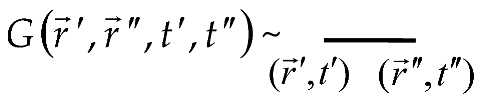
Let us associate the Green’s function $G({\overrightarrow{r}}^{\prime },{\overrightarrow{r}}^{″},t^{\prime },t^{″})$ with a straight line segment, to whose ends the points $({\overrightarrow{r}}^{\prime },t^{\prime })$ and $({\overrightarrow{r}}^{″},t^{″})$ are assigned [32]:

Let us associate the operator $L_s({\overrightarrow{r}}^{\prime },t^{\prime })$ with a vertical segment with dots at its ends:

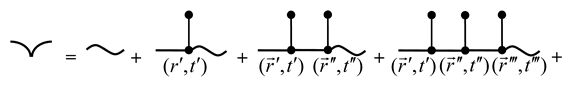
Let us associate the functions of the random concentration field $c(\overrightarrow{r},t)$ and the concentration field in a homogeneous body $c_h(\overrightarrow{r},t)$ with a tick and a wavy line, respectively:

The space–time positions $({\overrightarrow{r}}^{\prime },t^{\prime })$, $({\overrightarrow{r}}^{″},t^{″})$, where the lines visualizing $c(\overrightarrow{r},t)$, $c_h(\overrightarrow{r},t)$, $G(\overrightarrow{r},{\overrightarrow{r}}^{\prime },t,t^{\prime })$, and $L_s({\overrightarrow{r}}^{\prime },t^{\prime })$ merge together, are the vertices of a diagram. The integration is performed over the internal vertices’ coordinates. The total number of such vertices in the diagram determines its order. Such notations allow us to associate each term of the series (29) with a Feynman diagram. The first right-hand side element of (29) is represented by the diagram

and the second term of this formula corresponds to the diagram

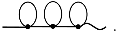
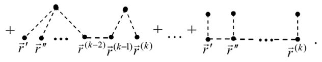
In the general case, a term of the order $n$ of the Neumann series for $c(\overrightarrow{r},t)$ has the form

$$\underset{n}{\underbrace{{\displaystyle \underset{0}{\overset{t}{\int }}{\displaystyle \underset{(V)}{\int }\hspace{0.17em}}}\dots {\displaystyle \underset{0}{\overset{t^{(n-1)}}{\int }}{\displaystyle \underset{(V)}{\int }\hspace{0.17em}}}}}G(\overrightarrow{r},t,{\overrightarrow{r}}^{\prime },t^{\prime })L_s({\overrightarrow{r}}^{\prime },t^{\prime })G({\overrightarrow{r}}^{\prime },t^{\prime },{\overrightarrow{r}}^{″},t^{″})\dots$$

$$\times L_s({\overrightarrow{r}}^{(n)},t^{(n)})c_h({\overrightarrow{r}}^{(n)},t^{(n)})d{\overrightarrow{r}}^{(n)}d{t}^{(n)}\dots d{\overrightarrow{r}}^{\prime }d{t}^{\prime }.$$

Therefore, the diagrams of the order $n$ contain $n$ lines of the Green’s function and $n$ lines of internal vertices $({\overrightarrow{r}}^{\prime },t^{\prime })$, …,$({\overrightarrow{r}}^{(n)},t^{(n)})$. At the same time, they always end in a wavy line $c_h(\overrightarrow{r})$ [30]:

Then, the series (29) in diagrammatical form will take the following form:

(31)

Averaging the random concentration field (29) over the ensemble of phase configurations yields the following analytical expression:

$$\langle c(\overrightarrow{r},t)\rangle =c_h(\overrightarrow{r},t)+{\displaystyle \underset{0}{\overset{t}{\int }}{\displaystyle \underset{(V)}{\int }}}G(\overrightarrow{r},{\overrightarrow{r}}^{\prime },t,t^{\prime })\langle L_s(\overrightarrow{r}\prime ,t^{\prime })\rangle c_h(\overrightarrow{r}\prime ,t^{\prime })d\overrightarrow{r}\prime d{t}^{\prime }$$

$$+{\displaystyle \underset{0}{\overset{t}{\int }}{\displaystyle \underset{(V)}{\int }{\displaystyle \underset{0}{\overset{t^{\prime }}{\int }}{\displaystyle \underset{(V)}{\int }G(\overrightarrow{r},{\overrightarrow{r}}^{\prime },t,t^{\prime })\langle L_s({\overrightarrow{r}}^{\prime },t^{\prime })G({\overrightarrow{r}}^{\prime },{\overrightarrow{r}}^{″},t^{\prime },t^{″})L_s({\overrightarrow{r}}^{″},t^{″})\rangle c_h({\overrightarrow{r}}^{″},t^{″})d{\overrightarrow{r}}^{″}d{t}^{″}d{\overrightarrow{r}}^{\prime }d{t}^{\prime }}}}}$$

$$+{\displaystyle \underset{0}{\overset{t}{\int }}{\displaystyle \underset{(V)}{\int }{\displaystyle \underset{0}{\overset{t^{\prime }}{\int }}{\displaystyle \underset{(V)}{\int }{\displaystyle \underset{0}{\overset{t^{″}}{\int }}{\displaystyle \underset{(V)}{\int }G(\overrightarrow{r},{\overrightarrow{r}}^{\prime },t,t^{\prime })\langle L_s({\overrightarrow{r}}^{\prime },t^{\prime })G({\overrightarrow{r}}^{\prime },{\overrightarrow{r}}^{″},t^{\prime },t^{″})}}}}}}$$

$$\times L_s({\overrightarrow{r}}^{″},t^{″})G({\overrightarrow{r}}^{″},{\overrightarrow{r}}^{‴},t^{″},t^{‴})L_s({\overrightarrow{r}}^{‴},t^{‴})\rangle c_h({\overrightarrow{r}}^{‴},t^{‴})d{\overrightarrow{r}}^{‴}d{t}^{‴}d{\overrightarrow{r}}^{″}d{t}^{″}d{\overrightarrow{r}}^{\prime }d{t}^{\prime }+\dots .$$

(32)

Considering the structure of the operator $L_s({\overrightarrow{r}}^{\prime },t^{\prime })$ (19), one needs to calculate the expressions of the type $〈{\eta }_{ij}({\overrightarrow{r}}^{\prime })〉$, $〈\delta \left({\overrightarrow{r}}^{\prime }-{\overrightarrow{r}}_{{\Gamma }_{ij}}\right)〉$, $〈{\eta }_{ij}({\overrightarrow{r}}^{\prime }){\eta }_{kl}({\overrightarrow{r}}^{″})〉$, $〈\delta \left({\overrightarrow{r}}^{\prime }-{\overrightarrow{r}}_{{\Gamma }_{ij}}\right)\delta \left({\overrightarrow{r}}^{″}-{\overrightarrow{r}}_{{\Gamma }_{kl}}\right)〉$, $〈{\eta }_{ij}\left({\overrightarrow{r}}^{\prime }\right)\delta \left({\overrightarrow{r}}^{″}-{\overrightarrow{r}}_{{\Gamma }_{kl}}\right)〉$, etc. That is, to calculate the averaged concentration field, it is required to determine the moments $〈{\eta }_{ij}({\overrightarrow{r}}^{\prime })\dots {\eta }_{kl}({\overrightarrow{r}}^{(n)})〉$, $〈\delta \left({\overrightarrow{r}}^{\prime }-{\overrightarrow{r}}_{{\Gamma }_{ij}}\right)\dots \delta \left({\overrightarrow{r}}^{(n)}-{\overrightarrow{r}}_{{\Gamma }_{kl}}\right)〉$, and $〈{\eta }_{ij}\left({\overrightarrow{r}}^{\prime }\right)\dots \delta \left({\overrightarrow{r}}^{(n)}-{\overrightarrow{r}}_{{\Gamma }_{kl}}\right)〉$ of all orders. With a general statistical distribution, this becomes a complex problem, and additionally, the issue of choosing an appropriate method for summing the averaged series arises. For example, in the case of a small volume fraction of inclusions for small diffusion coefficients, one can limit oneself to the “Born approximation” [33], i.e., considering only the first two terms of the Neumann series. Then, the problem is reduced to the case of perturbation of concentration fields by specified random sources.

In this case, the random field (first approximation) ${〈c〉}^{(1)}$ is a linear functional of fluctuations $\tilde{d}(\overrightarrow{r})=d(\overrightarrow{r})-〈d(\overrightarrow{r})〉$, $\tilde{\rho }(\overrightarrow{r})=\rho (\overrightarrow{r})-〈\rho (\overrightarrow{r})〉$. Therefore, each moment of ${〈c〉}^{(1)}$ is expressed linearly through the moments $\tilde{d}(\overrightarrow{r})$ and $\tilde{\rho }(\overrightarrow{r})$, having the same order.

The field of the averaged concentration in the Born approximation is defined as follows:

$${〈c(\overrightarrow{r},t)〉}^{(1)}=c^{(0)}(\overrightarrow{r},t)+{\displaystyle \underset{0}{\overset{t}{\int }}{\displaystyle \underset{(V)}{\int }G(\overrightarrow{r},{\overrightarrow{r}}^{\prime },t,t^{\prime })〈L_s({\overrightarrow{r}}^{\prime },t^{\prime })〉c^{(0)}({\overrightarrow{r}}^{\prime },t^{\prime })}}d{\overrightarrow{r}}^{\prime }d{t}^{\prime }.$$

(33)

In this case, $c^{(0)}(\overrightarrow{r},t)=c_h(\overrightarrow{r},t)$.

The correlation function (also known as autocorrelation), by its definition, is [34]

$${\psi }_c\left({\overrightarrow{r}}_1,{\overrightarrow{r}}_2,t\right)\equiv 〈c({\overrightarrow{r}}_1,t)c({\overrightarrow{r}}_2,t)〉-〈c({\overrightarrow{r}}_1,t)〉〈c({\overrightarrow{r}}_2,t)〉.$$

(34)

Here, if we use ${\overrightarrow{r}}_1={\overrightarrow{r}}_2=\overrightarrow{r}$, then we will obtain the variance of the random field $D[c]$ at the point $\overrightarrow{r}$:

$$D[c]\equiv {\sigma }_c^2(\overrightarrow{r},t)\equiv 〈{\left|\tilde{c}(\overrightarrow{r},t)\right|}^2〉=〈{\left[c(\overrightarrow{r},t)-〈c(\overrightarrow{r},t)〉\right]}^2〉.$$

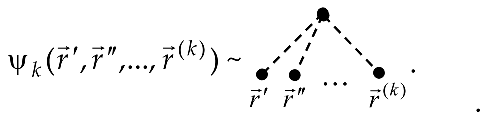
Relation (34) together with analogous expressions for higher-order moments of the field $c(\overrightarrow{r},t)$ yield a complete statistical solution of the problem. The statistical characteristics are described by cumulant (or correlation) functions of arbitrary order. We associate these functions with dashed lines, where the order of the cumulant function ${\psi }_k({\overrightarrow{r}}_1,{\overrightarrow{r}}_2,\dots ,{\overrightarrow{r}}_k)$ [34] matches the diagram order.

Because the concentration field is time deterministic, time appears as a parameter in cumulative functions.

In the general case, the moments from the operator $L_s$ that contains fluctuations $\tilde{d}(\overrightarrow{r})$ and $\tilde{\rho }(\overrightarrow{r})$ can be written down as [35]

$$〈L_s({\overrightarrow{r}}^{\prime },t^{\prime })\dots L_s({\overrightarrow{r}}^{(k)},t^{(k)})〉={\psi }_k({\overrightarrow{r}}^{\prime },\dots ,{\overrightarrow{r}}^{(k)})$$

$$+{\displaystyle \sum _{l=1}^k〈L_s({\overrightarrow{r}}^{(l)},t^{(l)})〉}〈L_s({\overrightarrow{r}}^{\prime },t^{\prime })\dots L_s({\overrightarrow{r}}^{(l-1)},t^{(l-1)})L_s({\overrightarrow{r}}^{(l+1)},t^{(l+1)})\dots L_s({\overrightarrow{r}}^{(k)},t^{(k)})〉+\dots$$

(35)

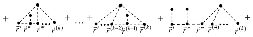
or in the form of diagrams

(36)

Note that expression (35) decomposes into the sum $k!$ of terms, in which the arguments ${\overrightarrow{r}}^{\prime }$, ${\overrightarrow{r}}^{″}$, …, ${\overrightarrow{r}}^{(k)}$ connected in every possible way. Therefore, at the time of averaging, we obtain $k!$ of diagrams of the $k$ order, in which $k$ vertices connect with each other in all possible ways. Note that, since integration occurs over the coordinates ${\overrightarrow{r}}^{\prime },{\overrightarrow{r}}^{″},\dots ,{\overrightarrow{r}}^{(k)}$ of the interior vertices, the analytical expression represented by the diagram has no dependency on the interior vertices’ coordinates. Thus, such coordinates are not indicated in the subsequent diagrams.

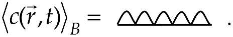
Let us introduce a graphical representation for the averaged concentration field in an inhomogeneous medium:

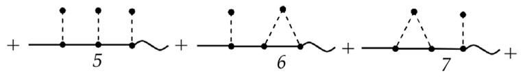
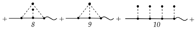
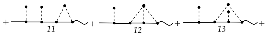
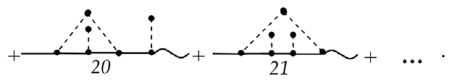
Then, the series (32) can be presented graphically as follows

(37)

Here, in addition to the terms written in (32), seven fourth-order terms (diagrams with four vertices) are also given.

Each Feynman diagram uniquely corresponds to an analytical expression and vice versa.

Certain diagrams comprising (37) include lower-order diagrams as fragments. For example, diagram 3 contains, as a fragment, diagram 2, and diagram 6 includes diagrams 2 and 4. This makes it possible to shorten the analytical expression.

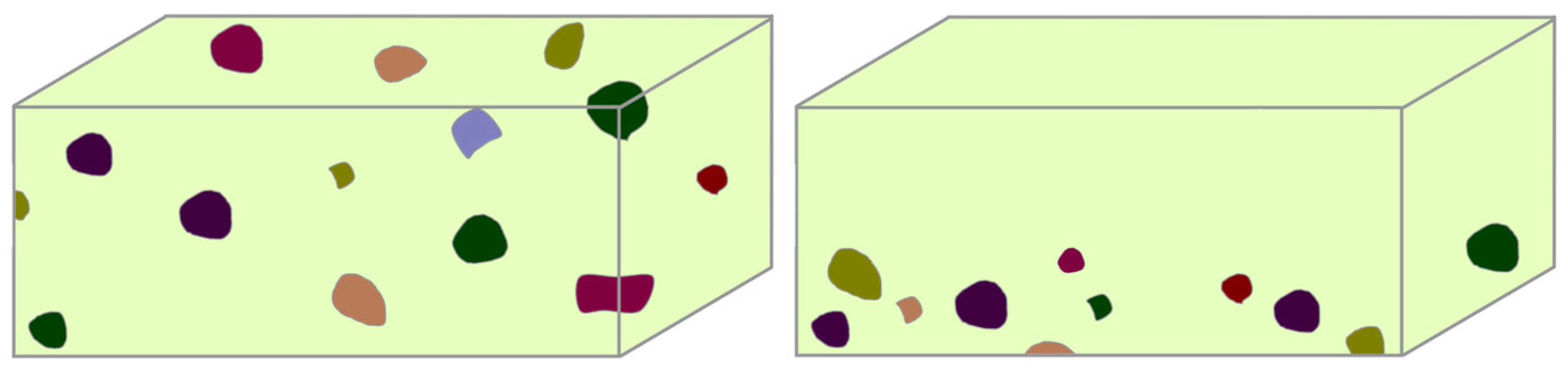
Let us consider the physical interpretation of Feynman diagrams. Diagram 1 from the series (37) describes the propagation of a concentration field from a source or from a surface (depending on the boundary conditions and the presence of internal mass sources) in a homogeneous medium. Diagram 2 describes the following process: the concentration field propagates from the source to point ${\overrightarrow{r}}^{\prime }$ as in a homogeneous medium. At point ${\overrightarrow{r}}^{\prime }$, the concentration field is perturbed because this point belongs to the inclusion or its boundary (${\overrightarrow{r}}^{\prime }$ belonging to the inclusion is determined by the averaged operator $〈L_s({\overrightarrow{r}}^{\prime })〉$, otherwise it is zero). Then, the perturbed field reaches point $\overrightarrow{r}$, where the observation takes place (Figure 2a).

Let us now consider the second-order diagrams. Diagram 3 represents the spread of the concentration field from the source to point ${\overrightarrow{r}}^{″}$, which is in the inclusion (operator $〈L_s({\overrightarrow{r}}^{″})〉$), where it experiences a perturbation; then, the perturbation field extends to point ${\overrightarrow{r}}^{\prime }$, which belongs to another inclusion (operator $〈L_s({\overrightarrow{r}}^{\prime })〉$ in analytical form) and experiences a second perturbation, after which, the twice perturbation field extends to the observation point $\overrightarrow{r}$ (Figure 2b). Diagram 4 differs from diagram 3 by the presence of the correlation function ${\psi }_2({\overrightarrow{r}}^{\prime },{\overrightarrow{r}}^{″})$, which indicates that the two perturbation points ${\overrightarrow{r}}^{\prime }$ and ${\overrightarrow{r}}^{″}$ are correlated, i.e., both perturbations occurred in the same heterogeneity (Figure 2c). All third-order diagrams 5–9 contain the functions $c_h({\overrightarrow{r}}^{‴},t^{‴})$, $G({\overrightarrow{r}}^{″},{\overrightarrow{r}}^{‴},t^{″},t^{‴})$, $G({\overrightarrow{r}}^{\prime },{\overrightarrow{r}}^{″},t^{\prime },t^{″})$, and $G(\overrightarrow{r},{\overrightarrow{r}}^{\prime },t,t^{\prime })$. This means that the concentration field has spread to the point $\overrightarrow{r}$ after perturbation in point ${\overrightarrow{r}}^{\prime }$, to point ${\overrightarrow{r}}^{\prime }$ after perturbation in point ${\overrightarrow{r}}^{″}$, and so on. Therefore, all these diagrams describe a triple perturbation of the concentration field. However, diagrams 5–9 are topologically different. Diagram 5 does not contain correlation functions, that is, three perturbations of the concentration field occurred in different inhomogeneities. Diagrams 6–8 contain correlation functions ${\psi }_2({\overrightarrow{r}}^{″},{\overrightarrow{r}}^{‴})$, ${\psi }_2({\overrightarrow{r}}^{\prime },{\overrightarrow{r}}^{″})$, and ${\psi }_2({\overrightarrow{r}}^{\prime },{\overrightarrow{r}}^{‴})$, respectively. This means that the field is perturbed three times in two inhomogeneities (Figure 3a–e).

Diagram 9 contains the cumulative function ${\psi }_3({\overrightarrow{r}}^{\prime },{\overrightarrow{r}}^{″},{\overrightarrow{r}}^{‴})$, that is, all three concentration field perturbations occur in a single inclusion.

Representing the solution of the initial-boundary value problem (17), (2), as a set of diagrams (37),allows for the transformationof the Neumann series using the topological features of the diagrams that contain solution.

The sum of series (32) can be represented as a sum involving a certain infinite subsequence of the same series. For this purpose, we classify the diagrams involved in (37) [31].

A diagram is termed weakly connected if, by breaking a certain one line $G$, it can be split into two separate diagrams. In expression (37), diagrams 3, 5–7, 10–13, 15, and 17–20 are weakly connected. The other diagrams, i.e., 1, 2, 4, 8, 9, 14, 16, and 21, are strongly connected. The diagrams obtained as a result of breaking $G$ lines can, in turn, be either strongly or weakly connected. If the set of “secondary” diagrams contains weakly connected diagrams, they can be split down into simpler diagrams. Following this procedure, we will end up with a certain number of strongly connected diagrams. The quantity of strongly connected diagrams resulting from the decomposition of a weakly connected diagram defines the “connectivity index” of the original diagram. Thus, in relation (37), the connectivity index of diagrams 3, 6, 7, 12, 13, 15, 19, and 20 is 2, and the connectivity index of diagrams 5, 11, 17, and 18 is 3. Let us assign the connectivity index 1 to the strongly connected diagrams.

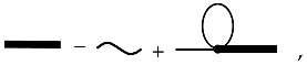
From the series (37), we extract all strongly connected diagrams, i.e., those that cannot be partitioned into two separate diagrams by cutting a single line $G$. As each diagram begins with a straight line and terminates with a wavy $c_h$ line, the sum of all strongly connected diagrams may be represented as

(38)

Analytically, we obtain

$${\overline{c}}^{(s.c.)}(\overrightarrow{r},t)={\displaystyle \underset{0}{\overset{t}{\int }}{\displaystyle \underset{(V)}{\int }}G(\overrightarrow{r},{\overrightarrow{r}}^{\prime },t,t^{\prime })\Sigma ({\overrightarrow{r}}^{\prime },t^{\prime })c_h({\overrightarrow{r}}^{\prime },t^{\prime })\hspace{0.17em}\hspace{0.17em}d{\overrightarrow{r}}^{\prime }d{t}^{\prime }},$$

(39)

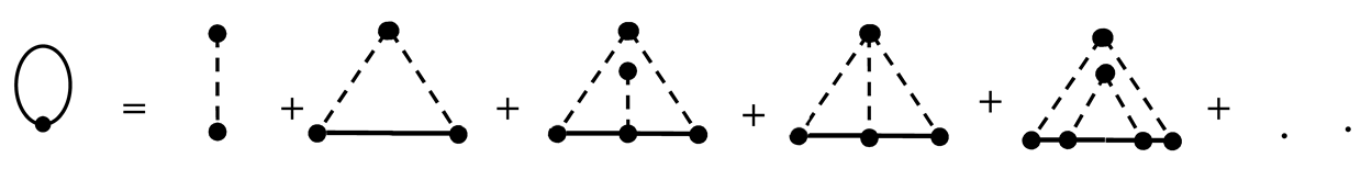
where $\Sigma (\overrightarrow{r},t)$ is the mass operator kernel:

$$\Sigma (\overrightarrow{r},t)=〈L_s(\overrightarrow{r},t)〉+{\displaystyle \underset{0}{\overset{t}{\int }}{\displaystyle \underset{(V)}{\int }G(\overrightarrow{r},{\overrightarrow{r}}^{\prime },t,t^{\prime }){\psi }_2(\overrightarrow{r},{\overrightarrow{r}}^{\prime })}d{\overrightarrow{r}}^{\prime }d{t}^{\prime }}$$

$$+{\displaystyle \underset{0}{\overset{t}{\int }}{\displaystyle \underset{0}{\overset{t^{\prime }}{\int }}{\displaystyle \underset{(V)}{\iint }G(\overrightarrow{r},{\overrightarrow{r}}^{\prime },t,t^{\prime })〈L_s({\overrightarrow{r}}^{\prime },t^{\prime })〉G({\overrightarrow{r}}^{\prime },{\overrightarrow{r}}^{″},t^{\prime },t^{″}){\psi }_2({\overrightarrow{r}}^{\prime },{\overrightarrow{r}}^{″})d{r}^{″}d{\overrightarrow{r}}^{\prime }d{t}^{″}d{t}^{\prime }}}}$$

$$+{\displaystyle \underset{0}{\overset{t}{\int }}{\displaystyle \underset{0}{\overset{t^{\prime }}{\int }}{\displaystyle \underset{(V)}{\iint }G(\overrightarrow{r},{\overrightarrow{r}}^{\prime },t,t^{\prime })G({\overrightarrow{r}}^{\prime },{\overrightarrow{r}}^{″},t^{\prime },t^{″}){\psi }_3(\overrightarrow{r},{\overrightarrow{r}}^{\prime },{\overrightarrow{r}}^{″})d{r}^{″}d{\overrightarrow{r}}^{\prime }d{t}^{″}d{t}^{\prime }}}}+\dots .$$

(40)

The mass operator kernel (40) can also be presented graphically:

(41)

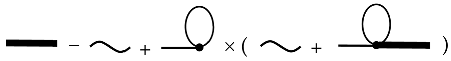
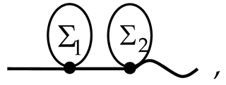
Let us focus on the sum of all the strongly connected diagrams with connectivity index = 1. Each of those diagrams possesses the following form:

(42)

where  and  denote arbitrary diagrams that are on the right side of (41).

Since, when the series (37) is being constructed, all variants of pairwise connection of the vertices are considered, the sum of all possible terms of the form (42) is

Here,  is the total sum of the mass operator kernel (40).

Similarly, the sum of all diagrams with a connectivity index of 3 has the form

and so on. Thus, we can present the averaged concentration field as a diagrammatic series:

(43)

Such a representation is distinct from the diagrammatic series (37), solely in the rearrangement of its elements.

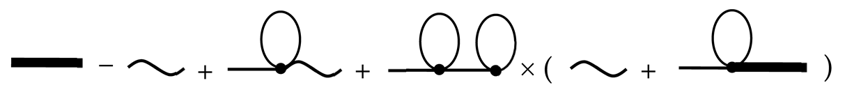
Let us verify that the series (41) is the solution of the following equation:

(44)

which is called the Dyson equation. We present the Dyson Equation (44) in analytical form:

$$〈c(\overrightarrow{r},t)〉=c_h(\overrightarrow{r},t)+{\displaystyle \underset{0}{\overset{t}{\int }}{\displaystyle \underset{(V)}{\int }}G(\overrightarrow{r},{\overrightarrow{r}}^{\prime },t,t^{\prime })\Sigma ({\overrightarrow{r}}^{\prime },t^{\prime })〈c({\overrightarrow{r}}^{\prime },t^{\prime })\hspace{0.17em}〉\hspace{0.17em}d{\overrightarrow{r}}^{\prime }d{t}^{\prime }}.$$

(45)

Let us show that the series (43) is a solution of equation (45). Let us apply the method of successive iterations. Relation (44) is substituted into the expression for the averaged concentration field $〈c(\overrightarrow{r},t)〉$ into the right-hand side of (44). We obtain

Again, by substituting the right-hand side of the resulting relation into the right side of (44), we obtain

If we continue the iterations, we will obtain the series (43). Similar calculations can be carried out in analytical form if we proceed from Equation (45). In this case, we will obtain the expansion (43) in analytical form, namely

$$〈c(\overrightarrow{r},t)〉=c_h(\overrightarrow{r},t)+{\displaystyle \underset{0}{\overset{t}{\int }}{\displaystyle \underset{(V)}{\int }}G(\overrightarrow{r},{\overrightarrow{r}}^{\prime },t,t^{\prime })\Sigma ({\overrightarrow{r}}^{\prime },t^{\prime })c_h({\overrightarrow{r}}^{\prime },t^{\prime })\hspace{0.17em}d{\overrightarrow{r}}^{\prime }d{t}^{\prime }}+$$

$$+{\displaystyle \underset{0}{\overset{t}{\int }}{\displaystyle \underset{0}{\overset{t^{\prime }}{\int }}{\displaystyle \underset{(V)}{\iint }G(\overrightarrow{r},{\overrightarrow{r}}^{\prime },t,t^{\prime })\Sigma ({\overrightarrow{r}}^{\prime },t^{\prime })G({\overrightarrow{r}}^{\prime },{\overrightarrow{r}}^{″},t^{\prime },t^{″})\Sigma ({\overrightarrow{r}}^{″},t^{″})c_h({\overrightarrow{r}}^{″},t^{″})d{\overrightarrow{r}}^{″}d{\overrightarrow{r}}^{\prime }d{t}^{″}d{t}^{\prime }}}}+$$

$$+{\displaystyle \underset{0}{\overset{t}{\int }}{\displaystyle \underset{0}{\overset{t^{\prime }}{\int }}{\displaystyle \underset{0}{\overset{t^{″}}{\int }}{\displaystyle \underset{(V)}{\iiint }G(\overrightarrow{r},{\overrightarrow{r}}^{\prime },t,t^{\prime })\Sigma ({\overrightarrow{r}}^{\prime },t^{\prime })G({\overrightarrow{r}}^{\prime },{\overrightarrow{r}}^{″},t^{\prime },t^{″})\Sigma ({\overrightarrow{r}}^{″},t^{″})G({\overrightarrow{r}}^{″},{\overrightarrow{r}}^{‴},t^{″},t^{‴})}}\times }}$$

$$\times \Sigma ({\overrightarrow{r}}^{‴},t^{‴})c_h({\overrightarrow{r}}^{‴},t^{‴})d{\overrightarrow{r}}^{‴}d{\overrightarrow{r}}^{″}d{\overrightarrow{r}}^{\prime }d{t}^{‴}d{t}^{″}d{t}^{\prime }.$$

(46)

Equation (45), assuming $\Sigma (\overrightarrow{r},t)$ is known, is an integral equation in relation to $〈c(\overrightarrow{r},t)〉$, which can be solved in some cases. At that, we will obtain an explicit expression of the averaged concentration field $〈c(\overrightarrow{r},t)〉$ through the mass operator kernel $\Sigma (\overrightarrow{r},t)$, i.e., the sum of the series (32) is given using the quantity ${\overline{c}}^{(s.c.)}(\overrightarrow{r},t)$ (39), which is a certain subsequence of the same series.

$\Sigma (\overrightarrow{r},t)$, as the operator in the general case and as the function in a given instance, is not known exactly. In the approximate case, for example, the sum of the first few terms of the series (46) can be used as this operator (function). In the case of the Bourret approximation [31],representing the first-order term in the series expansion of the mass operator, we have

(47)

Considering the structure of the operator $L_s(\overrightarrow{r},t)$ (19), the expression for $〈L_s(\overrightarrow{r},t)〉$ can be presented at non-ideal mass contact conditions as

$$〈L_s(\overrightarrow{r},t)〉={\displaystyle \sum _{j=1}^N{\displaystyle \sum _{i=1}^{n_j}〈{\eta }_{ji}(\overrightarrow{r})〉}\left[({\rho }_0-{\rho }_j)\frac{\partial }{\partial t}-(d_0-d_j)\Delta \right]}$$

$$+{\displaystyle \frac{1}{2}}{\displaystyle \sum _{j=0}^N{\displaystyle \sum _{i=1}^{n_j}{\left[d(\overrightarrow{r})\right]}_{{\Gamma }_{ji}}{\left[\overrightarrow{\nabla }\dots \right]}_{{\Gamma }_{ji}}}}〈\delta \left(\overrightarrow{r}-{\overrightarrow{r}}_{{\Gamma }_{ji}}\right)〉+{\displaystyle \frac{1}{2}}{\displaystyle \sum _{j=0}^N{\displaystyle \sum _{i=1}^{n_j}{\left[d(\overrightarrow{r})\right]}_{{\Gamma }_{ji}}{\left[\dots \right]}_{{\Gamma }_{ji}}}}〈\overrightarrow{\nabla }\delta \left(\overrightarrow{r}-{\overrightarrow{r}}_{{\Gamma }_{ji}}\right)〉$$

$$+{\displaystyle \frac{1}{2}}{\displaystyle \sum _{j=0}^N{\displaystyle \sum _{i=1}^{n_j}{\left[d(\overrightarrow{r})\right]}_{{\Gamma }_{ji}}{\left[\dots \right]}_{{\Gamma }_{ji}}}}〈{\delta }^2\left(\overrightarrow{r}-{\overrightarrow{r}}_{{\Gamma }_{ji}}\right)〉,$$

(48)

and at ideal contact conditions as

$$〈L_s(\overrightarrow{r},t)〉={\displaystyle \sum _{j=1}^N{\displaystyle \sum _{i=1}^{n_j}〈{\eta }_{ji}(\overrightarrow{r})〉}\left[({\rho }_0-{\rho }_j)\frac{\partial }{\partial t}-(d_0-d_j)\Delta \right]}.$$

(49)

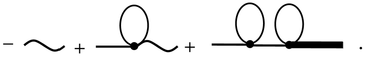
The Bourret approximation for the averaged concentration field $〈c(\overrightarrow{r},t)〉$ is graphically designated as

(50)

If, in the diagrammatic Formula (43), we put diagram (47) instead of $\Sigma (\overrightarrow{r},t)$, this leads to the diagrammatic representation of ${〈c(\overrightarrow{r},t)〉}_B$ as

and the analytical form as

$$\begin{gathered} {〈c(\overrightarrow{r},t)〉}_B=c_h(\overrightarrow{r},t)+{\displaystyle \underset{0}{\overset{t}{\int }}{\displaystyle \underset{(V)}{\int }G(\overrightarrow{r},{\overrightarrow{r}}^{\prime },t,t^{\prime })〈L_s({\overrightarrow{r}}^{\prime },t^{\prime })〉c_h({\overrightarrow{r}}^{\prime },t^{\prime })d{\overrightarrow{r}}^{\prime }d{t}^{\prime }}} \\ +{\displaystyle \underset{0}{\overset{t}{\int }}{\displaystyle \underset{0}{\overset{t^{\prime }}{\int }}{\displaystyle \underset{(V)}{\iint }G(\overrightarrow{r},{\overrightarrow{r}}^{\prime },t,t^{\prime })〈L_s({\overrightarrow{r}}^{\prime },t^{\prime })〉G({\overrightarrow{r}}^{\prime },{\overrightarrow{r}}^{″},t^{\prime },t^{″})〈L_s({\overrightarrow{r}}^{″},t^{″})〉c_h({\overrightarrow{r}}^{″},t^{″})d{\overrightarrow{r}}^{″}d{\overrightarrow{r}}^{\prime }d{t}^{″}d{t}^{\prime }+\dots }}} \end{gathered}$$

(51)

If a randomly inhomogeneous medium is not only statistically homogeneous but also statistically isotropic, then Formula (51) can be simplified by transitioning to spherical coordinates and performing integration over angular variables [31].

6. Equation for the Averaged Concentration Field in a Multiphase Randomly Inhomogeneous Medium

Now, let us obtain an equation whose solution is the averaged concentration field $〈c(\overrightarrow{r},t)〉$.

Let us apply operator $L_0(\overrightarrow{r},t)={\rho }_0{\displaystyle \frac{\partial }{\partial t}}-d_0\Delta$ to Dyson Equation (45). We obtain

$$\begin{gathered} \left[{\rho }_0{\displaystyle \frac{\partial }{\partial t}}-d_0\Delta \right]〈c(\overrightarrow{r},t)〉=\left[{\rho }_0{\displaystyle \frac{\partial }{\partial t}}-d_0\Delta \right]c_h(\overrightarrow{r},t) \\ +{\displaystyle \underset{0}{\overset{t}{\int }}{\displaystyle \underset{(V)}{\int }}\left[{\rho }_0\frac{\partial }{\partial t}-d_0{\Delta }_{\overrightarrow{r}}\right]G(\overrightarrow{r},{\overrightarrow{r}}^{\prime },t,t^{\prime })\Sigma ({\overrightarrow{r}}^{\prime },t^{\prime })〈c({\overrightarrow{r}}^{\prime },t^{\prime })\hspace{0.17em}〉\hspace{0.17em}d{\overrightarrow{r}}^{\prime }d{t}^{\prime }}. \end{gathered}$$

(52)

According to Formula (21), the first term of Equation (52) is $L_0(\overrightarrow{r},t)c_h(\overrightarrow{r},t)=0$, and from relation (23), we conclude that $L_0(\overrightarrow{r},t)G(\overrightarrow{r},{\overrightarrow{r}}^{\prime },t,t^{\prime })=\delta (t-t^{\prime })\delta (\overrightarrow{r}-{\overrightarrow{r}}^{\prime })$.

Considering the properties of the delta function, after integration, we arrive at

$$\left[{\rho }_0{\displaystyle \frac{\partial }{\partial t}}-d_0\Delta -\Sigma (\overrightarrow{r},t)\right]〈c(\overrightarrow{r},t)〉=0.$$

(53)

The obtained equation is a partial differential equation with respect to the averaged random field of impurity concentration.

For the Bourret approximation (47), Equation (53) can be written as

$${\rho }_0{\displaystyle \frac{\partial {〈c(\overrightarrow{r},t)〉}_B}{\partial t}}-d_0\Delta {〈c(\overrightarrow{r},t)〉}_B-〈L_s(\overrightarrow{r},t)〉{〈c(\overrightarrow{r},t)〉}_B=0.$$

(54)

Let us take into account that the averaged concentration field is a continuous function in all spatial coordinates. Accordingly, we obtain

$$〈L_s(\overrightarrow{r},t)〉{〈c(\overrightarrow{r},t)〉}_B={\displaystyle \sum _{j=1}^N{\displaystyle \sum _{i=1}^{n_j}〈{\eta }_{ji}(\overrightarrow{r})〉}\left[({\rho }_0-{\rho }_j)\frac{\partial {〈c(\overrightarrow{r},t)〉}_B}{\partial t}-(d_0-d_j)\Delta {〈c(\overrightarrow{r},t)〉}_B\right]}$$

$$+{\displaystyle \frac{1}{2}}{\displaystyle \sum _{j=0}^N{\displaystyle \sum _{i=1}^{n_j}{\left[\overrightarrow{\nabla }{〈c(\overrightarrow{r},t)〉}_B\right]}_{{\Gamma }_{ji}}}}〈{\left[d(\overrightarrow{r})\right]}_{{\Gamma }_{ji}}\delta \left(\overrightarrow{r}-{\overrightarrow{r}}_{{\Gamma }_{ji}}\right)〉.$$

(55)

If, in addition, the first derivatives with respect to ${\overrightarrow{r}}^{\prime }$ do not have jumps, then we obtain

$$〈L_s(\overrightarrow{r},t)〉{〈c(\overrightarrow{r},t)〉}_B={\displaystyle \sum _{j=1}^N{\displaystyle \sum _{i=1}^{n_j}〈{\eta }_{ji}(\overrightarrow{r})〉}\left[({\rho }_0-{\rho }_j)\frac{\partial {〈c(\overrightarrow{r},t)〉}_B}{\partial t}-(d_0-d_j)\Delta {〈c(\overrightarrow{r},t)〉}_B\right]}.$$

(56)

After substituting relation (56) into Equation (55), we have

$${\rho }_0{\displaystyle \frac{\partial {〈c(\overrightarrow{r},t)〉}_B}{\partial t}}-d_0\Delta {〈c(\overrightarrow{r},t)〉}_B$$

$$-{\displaystyle \sum _{j=1}^N{\displaystyle \sum _{i=1}^{n_j}〈{\eta }_{ji}(\overrightarrow{r})〉}\left[({\rho }_0-{\rho }_j)\frac{\partial {〈c(\overrightarrow{r},t)〉}_B}{\partial t}-(d_0-d_j)\Delta {〈c(\overrightarrow{r},t)〉}_B\right]}=0.$$

(57)

The resulting equation (57) is a second-order partial differential equation with respect to the concentration field ${〈c(\overrightarrow{r},t)〉}_B$ averaged over the ensemble of phase configurations for the Bourret approximation. Moreover, the coefficients near the first two terms are the characteristics of the matrix, and the coefficients near the last term of the equation are the deviations of the corresponding coefficients of phase j from the characteristics of the matrix.

Equation (57) can be rewritten as

$$\left[{\rho }_0-{\displaystyle \sum _{j=1}^N{\displaystyle \sum _{i=1}^{n_j}〈{\eta }_{ji}(\overrightarrow{r})〉}({\rho }_0-{\rho }_j)}\right]{\displaystyle \frac{\partial {〈c(\overrightarrow{r},t)〉}_B}{\partial t}}$$

$$-\left[d_0-{\displaystyle \sum _{j=1}^N{\displaystyle \sum _{i=1}^{n_j}〈{\eta }_{ji}(\overrightarrow{r})〉}(d_0-d_j)}\right]\Delta {〈c(\overrightarrow{r},t)〉}_B=0.$$

(58)

Let the phases be uniformly distributed within the body. Then, after averaging the structure function (10), we obtain

$${\displaystyle \sum _{i=1}^{n_j}〈{\eta }_{ji}(\overrightarrow{r})〉}={\displaystyle \frac{V_j}{V}}=v_j.$$

(59)

As a result, Equation (58) will take the following form:

$$\left[{\rho }_0-{\displaystyle \sum _{j=1}^N{v}_j({\rho }_0-{\rho }_j)}\right]{\displaystyle \frac{\partial {〈c(\overrightarrow{r},t)〉}_B}{\partial t}}-\left[d_0-{\displaystyle \sum _{j=1}^N{v}_j(d_0-d_j)}\right]\Delta {〈c(\overrightarrow{r},t)〉}_B=0.$$

(60)

In a specific case, for a two-phase body, (60) is equivalent to

$$\left[{\rho }_0-v_1({\rho }_0-{\rho }_1)\right]{\displaystyle \frac{\partial {〈c(\overrightarrow{r},t)〉}_B}{\partial t}}-\left[d_0-v_1(d_0-d_1)\right]\Delta {〈c(\overrightarrow{r},t)〉}_B=0,$$

(61)

and in the case of a three-phase body, it is equivalent to

$$\left[{\rho }_0-v_1({\rho }_0-{\rho }_1)-v_2({\rho }_0-{\rho }_2)\right]{\displaystyle \frac{\partial {〈c(\overrightarrow{r},t)〉}_B}{\partial t}}$$

$$-\left[d_0-v_1(d_0-d_1)-v_2(d_0-d_2)\right]\Delta {〈c(\overrightarrow{r},t)〉}_B=0.$$

(62)

Equations (60)–(62) together with the original boundary conditions can be solved analytically.

7. Impurity Diffusion in a Two-Phase Randomly Inhomogeneous Layer

To study the influence of inhomogeneities on the behavior and the values of the averaged concentration field, we consider the case of impurity mass transfer in a two-phase randomly inhomogeneous layer. The phases in the body are arranged according to a uniform probability distribution. The obtained averaged concentration field will be compared with solutions of similar problems of impurity diffusion in a homogeneous layer with matrix characteristics and in a homogeneous layer with parameters averaged over the body volume.

The diffusion of impurity in a layer of thickness $z_0$ is described by an initial-boundary value problem based on Equation (61) in the one-dimensional case, i.e.,

$$\left[{\rho }_0-v_1({\rho }_0-{\rho }_1)\right]{\displaystyle \frac{\partial {〈c(z,t)〉}_B}{\partial t}}-\left[d_0-v_1(d_0-d_1)\right]{\displaystyle \frac{{\partial }^2{〈c(z,t)〉}_B}{\partial z^2}}=0,$$

(63)

$${\left.{〈c(z,t)〉}_B\right|}_{t=0}=0, {\left.{〈c(z,t)〉}_B\right|}_{z=0}={\tilde{c}}_1\equiv const, {\left.{〈c(z,t)〉}_B\right|}_{z=z_0}={\tilde{c}}_2\equiv const.$$

(64)

The diffusion of an impurity in a layer with volume-averaged characteristics is governed by the following equation:

$$\overline{\rho }{\displaystyle \frac{\partial \overline{c}(z,t)}{\partial t}}-\overline{d}{\displaystyle \frac{{\partial }^2\overline{c}(z,t)}{\partial z^2}}=0$$

(65)

with the boundary conditions (64). Here, $\overline{\rho }=v_0{\rho }_0+v_1{\rho }_1$, $\overline{d}=v_0{d}_0+v_1{d}_1$.

The equation of the diffusion of an impurity in a homogeneous layer with matrix characteristics has the form

$${\rho }_0{\displaystyle \frac{\partial c_h(z,t)}{\partial t}}-d_0{\displaystyle \frac{{\partial }^2{c}_h(z,t)}{\partial z^2}}=0.$$

(66)

Boundary conditions remain the same.

Note that the partial differential equation for the averaged concentration (63) can be considered as a certain homogenized diffusion equation, the coefficients of which differ significantly from the averaged ones of Equation (65). At the same time, the operators of these equations have the same structure.

Let us investigate the solution to the problem (63) and (64) and compare it with the solutions of the initial-boundary value problems (64), (65) and (60), (64).

The solution to the problem (63) and (64) is the following [25]:

$${〈c(z,t)〉}_B={\tilde{c}}_1\left(1-{\displaystyle \frac{z}{z_0}}\right)+{\tilde{c}}_2{\displaystyle \frac{z}{z_0}}-$$

$$-{\displaystyle \frac{2}{{\rho }_0{z}_0}}{\displaystyle \sum _{n=1}^{\infty }\frac{1}{z_n}\left({\tilde{c}}_1+{(-1)}^{n+1}{\tilde{c}}_2\right)e^{-\frac{\left[d_0-v_1(d_0-d_1)\right]z_n^{2}t}{{\rho }_0-v_1({\rho }_0-{\rho }_1)}}\sin (z_{n}z)},$$

(67)

where $z_n=n\pi /z_0$, $n=1,\hspace{0.17em}2,\hspace{0.17em}\dots$.

Let us show the graphs of the average concentration of impurity migrating in a layer. Numerical calculations were carried out in dimensionless variables

$$\xi =z/z_0, \tau =dt/\rho z_0^2.$$

(68)

The following parameter values were used as baselines: ${\rho }_0=1$, ${\rho }_1=1.1$, $d_0=1$, $d_1=0.5$ and $1.5$, $v_1=0.1$, ${\xi }_0=1$, ${\tilde{c}}_1=1$, and ${\tilde{c}}_2=0.05$. Calculations were carried out using Formula (67). The accuracy when summing rows in formulas was ${10}^{-12}$. Along the ordinate axis, the function $〈c(\xi ,\tau )〉/{\tilde{c}}_1$, that is the concentration function normalized to its boundary value $\xi =0$ (64), was laid down.

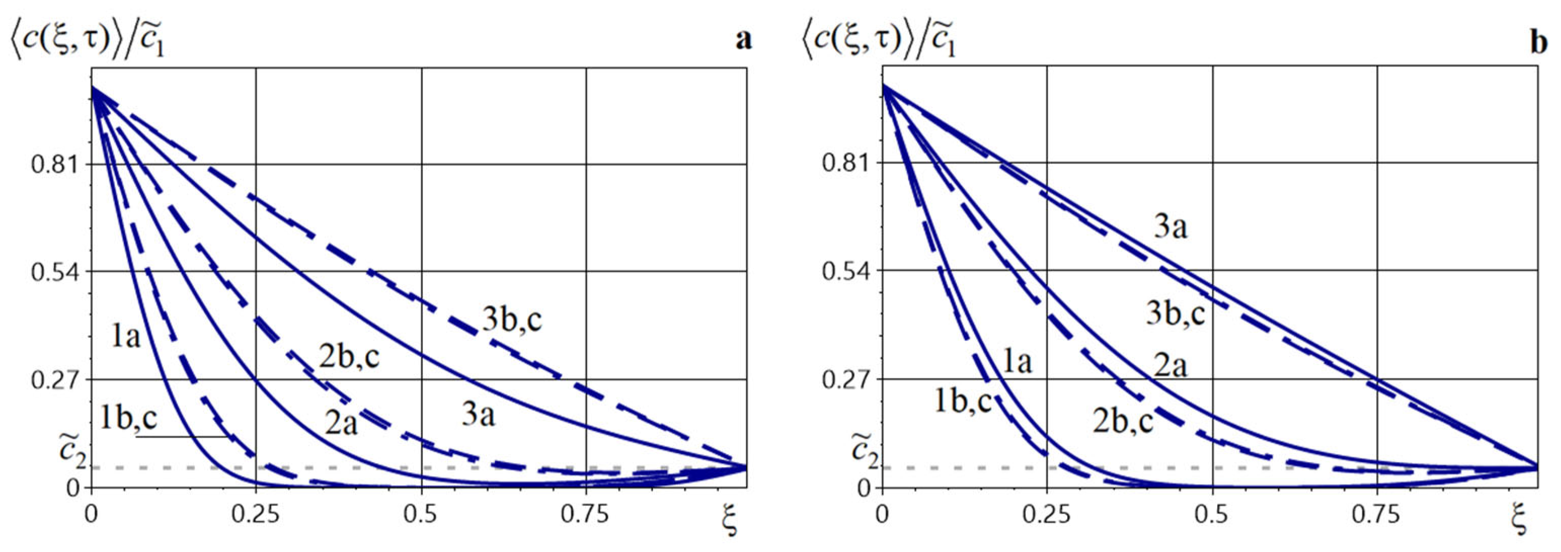
Figure 4 illustrates the distributions of concentration $〈c(\xi ,\tau )〉/{\tilde{c}}_1$ averaged over the ensemble of phase configurations (curves a, solid lines), concentrations in a layer with volume-averaged characteristics (curves b, dash-dotted lines), and concentrations in a homogeneous layer with matrix characteristics (c curves, dashed lines) at the moments of time $\tau =0.01$ (curves 1), $\tau =0.05$ (curves 2), and $\tau =0.25$ (curves 3). Here, Figure 4a is constructed for $d_1=0.5$ and Figure 4b for $d_1=1.5$. The same applies to the figures a and b below unless stated otherwise.

Figure 5 presents the graphs of the average particle concentration for different values of the kinetic coefficient in inclusions $d_1$ = 0.01, 0.5, 1.5, 5, and 20 (curves 1–5, respectively) for $\tau =0.05$ (Figure 5a) and $\tau =0.25$ (Figure 5b). Here, and further on, the dashed lines correspond to the impurity concentration in the body possessing the characteristics of the base phase.

Figure 6 demonstrates the behavior of the function $〈c(\xi ,\tau )〉/{\tilde{c}}_1$ depending on different values of the inclusion’s volume fraction of $v_1=$0.01, 0.05, 0.1, 0.2, and 0.3 (curves 1–5) for $d_1=0.5$ (Figure 6a) and $d_1=1.5$ (Figure 6b). Figure 7 illustrates the graphs of the averaged concentration $〈c(\xi ,\tau )〉/{\tilde{c}}_1$ and particle concentrations in the matrix $c^{(0)}(\xi ,\tau )/{\tilde{c}}_1$ for different values of the searched function on the bottom surface of the layer ${\tilde{c}}_2=$ 0.01, 0.05, 0.25, and 0.5 (curves 1–4), $d_1=0.5$ (Figure 7a), and $d_1=1.5$ (Figure 7b).

It should be noted that the use of the impurity diffusion model to calculate the concentration averaged over the ensemble of phase configurations in a two-phase layer in which the phases are uniformly distributed leads to results that are significantly different from those obtained using diffusion models with volume-averaged characteristics and with matrix characteristics (Figure 4). At the same time, the difference between the solutions of problems, (64), (65) and (64), (66) is insignificant and amounts to 7% for the time moment $\tau =0.05$. With increasing diffusion time, the concentration functions in all models increase until they reach a steady state (curves 3b, c in Figure 4a and curves 3a in Figure 4b), and the difference between them is decreasing. If the values of the diffusion coefficient in inclusions are smaller than in the matrix, i.e., $d_1<d_0$, the values of the function $〈c(\xi ,\tau )〉$ are always smaller than those of the concentration functions calculated using other models (Figure 4a,b). For $d_1>d_0$, the opposite situation is observed—the values of the concentration averaged over the ensemble of phase configurations are always higher than the solutions of problems (64), (65) and (64), (66) (Figure 4b).

Let us also remark that the greater the ratio $d_1/d_0$, the faster the function $〈c(\xi ,\tau )〉$ reaches a steady state (Figure 5). Thus, the time needed to reach the steady state regime of the concentration function for $d_1/d_0=20$ is ${\tau }_{st}=0.02$ and for $d_1/d_0=0.5$ is ${\tau }_{st}=1.1$.

Changing the volume fraction of inclusions has a negligible effect on the value of the function $〈c(\xi ,\tau )〉$ (Figure 6). Therefore, the difference between ${\left.〈c(\xi ,\tau )〉\right|}_{v_1=0.01}$ and ${\left.〈c(\xi ,\tau )〉\right|}_{v_1=0.3}$, that is, when $v_1$ is increased by 30 times, reaches 25%. The value of the concentration function ${\tilde{c}}_2$ at the bottom surface of the layer affects its behavior in the lower half of the body (Figure 7).The largest differences between the average impurity concentration in the layer and the matrix characteristics are observed in the interval $\xi \in [0.6,\hspace{0.17em}0.7]$ (Figure 7).

As an example of a real diffusion process that can be simulated by the methods developed in this article, we present graphs of the averaged hydrogen concentration field in a two-phase iron–copper body. Consider the problem of hydrogen migration in the composite material $Fe-Cu$, taking iron as the base phase. The diffusion coefficients of hydrogen were assumed as [36,37]: in iron $d_{Fe}=1.8\times {10}^{-11}$ m²/s, in copper $d_{Cu}=4.34\times {10}^{-10}$ m²/s; the densities of iron ${\rho }_{Fe}=7.8\times {10}^3$ kg/m³ and copper ${\rho }_{Cu}=8.39\times {10}^3$ kg/m³ From these values, one obtains the dimensionless parameters ${\widehat{d}}_1=d_{Cu}/d_{Fe}=24.11$ and ${\widehat{\rho }}_1={\rho }_{Cu}/{\rho }_{Fe}=1.145$.

Illustrated in Figure 8 is the behavior of the averaged hydrogen-concentration field for $v_{Cu}=0.05$ (Figure 8a) and $v_{Cu}=0.15$ (Figure 8b) in the composite material $Fe-Cu$. Curves 1–3 correspond to the dimensionless times $\tau =0.01,\hspace{0.17em}0.05,\hspace{0.17em}0.25$, respectively.

It should be noted that, as the volume fraction of copper increases, the averaged hydrogen-concentration field reaches its steady-state regime more rapidly (Figure 8).

8. Conclusions

The modeling of the process of impurity particle diffusion in a multiphase randomly inhomogeneous body is presented in this paper. The diffusion process is described with the help of mass balance equations for components of a thermodynamic system. Non-ideal contact conditions in terms of impurity concentration are set at interphase boundaries. Based on the mass balance equation for the entire body, a stochastic partial differential equation of the impurity mass transfer for the entire body is obtained. The equation operator contains jump discontinuities of the searched function and its derivative at random interfaces.

The resulting boundary value problem is assigned an integro-differential equation featuring a random kernel, the solution of which is obtained as an integral Neumann series. To study its structure, a graphical representation of the series elements in the form of R. Feynman diagrams is introduced. The physical interpretation of these diagrams is given.

The random concentration field is averaged over an ensemble of phase configurations. Employing the topological properties of diagrams, the averaged Neumann series is expressed as the sum of a certain infinite subsequence of the same series. A classification of diagrams is proposed, with grouping into two types: strongly and weakly connected. The kernel of the mass operator is constructed based on the sum of all strongly connected diagrams.

Usage of the Feynman diagram technique enabled us to obtain the Dyson integro-differential equation for the averaged concentration field in graphical and analytical forms. A simplified operator of the Dyson equation in the case of the Bourret approximation was constructed. However, for a more accurate description of the processes, it is advisable to consider the case with two terms in the mass operator kernel approximation. This approach will allow for corrections of the results that consider a more complex structure of interactions and can provide higher accuracy of calculations.

A partial differential equation for the averaged concentration field is specified for the case of N phases uniformly distributed in the body region. The differential equation of mass transfer is detailed for two- and three-phase bodies.

The behavior of the averaged impurity concentration in a two-phase stochastically inhomogeneous layer with a uniform distribution of phases under initial and boundary conditions of the first kind is investigated. The found averaged concentration field was compared with solutions of similar mass transfer problems in a homogeneous layer with base phase coefficients and in a homogeneous layer with characteristics averaged over the body volume. It is shown that the values of the averaged concentration field differ significantly from the solutions to homogeneous initial-boundary value problems, but this difference decreases over time as the diffusion process progresses. It has been found that, if the inclusions’ kinetic diffusion coefficient is greater than in the base phase, the values of the concentration averaged over the ensemble of phase configurations are always higher than the solutions of homogeneous problems. Otherwise, the values of the averaged concentration field are always lower than the concentrations calculated using other models.

It is advisable to use this approach in the future to investigate the correlations of stochastic concentration fields, obtain nonlocal equations for coherence functions, and investigate mass transfer processes in stochastically inhomogeneous bodies under the theory of binary systems for different probability distributions of phases. This will allow for an assessmentof the sensitivity of the obtained results to assumptions regarding the distribution of parameters and make the model more general and suitable for a wide class of problems.

References

1. Harlander, R.V.; Martinez, J.-P. The development of computational methods for Feynman diagrams. Eur. Phys. J. H 2024, 49, 4. [Google Scholar] [CrossRef]
2. Dorato, M.; Rossanese, E. The nature of representation in Feynman diagrams. Perspect. Sci. 2018, 26, 443–458. [Google Scholar] [CrossRef]
3. Stöltzner, M. Feynman diagrams: Modeling between physics and mathematics. Perspect. Sci. 2018, 26, 482–500. [Google Scholar] [CrossRef]
4. Brown, J.R. How do feynman diagrams work? Perspect. Sci. 2018, 26, 423–442. [Google Scholar] [CrossRef]
5. Stöltzner, M. Feynman Diagrams as Models. Math. Intell. 2017, 39, 46–51. [Google Scholar] [CrossRef]
6. Cangiotti, N.; Nappo, F. Reasoning by Analogy in Mathematical Practice. Philos. Math. 2023, 31, 176–215. [Google Scholar] [CrossRef]
7. Forgione, M. Feynman diagrams: Visualization of phenomena and diagrammatic representation. Eur. J. Philos. Sci. 2024, 14, 48. [Google Scholar] [CrossRef]
8. Zajac, S.; Geary, C.; Andersen, E.S.; Dabrowski-Tumanski, P.; Sulkowska, J.I.; Sułkowski, P. Genus trace reveals the topological complexity and domain structure of biomolecules. Sci. Rep. 2018, 8, 17537. [Google Scholar] [CrossRef]
9. Antczak, M.; Popenda, M.; Zok, T.; Zurkowski, M.; Adamiak, R.W.; Szachniuk, M. New algorithms to represent complex pseudo knotted RNA structures in dot-bracket notation. Bioinformatics 2017, 34, 1304–1312. [Google Scholar] [CrossRef]
10. Pal, A.; Bhattacharjee, J.K. Perturbation theory for stochastic nonlinear oscillators and Feynman diagram. Ann. Phys. 2023, 459, 169495. [Google Scholar] [CrossRef]
11. Yamazaki, K. A note on the applications of Wick products and Feynman diagrams in the study of singular partial differential equations. J. Comput. Appl. Math. 2021, 388, 113338. [Google Scholar] [CrossRef]
12. Mahajan, R.; Singh, V.A. Feynman Diagrams: A Toy Example. Resonance 2019, 24, 653–659. [Google Scholar] [CrossRef]
13. Gopalakrishna, K.; Labelle, P.; Shramchenko, V. Feynman diagrams, ribbon diagrams, and topological recursion of Eynard-Orantin. J. High Energy Phys. 2018, 2018, 162. [Google Scholar] [CrossRef]
14. Thomas, P.; Fleck, C.; Grima, R.; Popović, N. System size expansion using Feynman rules and diagrams. J. Phys. A Math. Theor. 2014, 47, 455007. [Google Scholar] [CrossRef]
15. Kalmykov, M.Y.; Kniehl, B.A. Mellin-Barnes representations of Feynman diagrams, linear systems of differential equations, and polynomial solutions. Phys. Lett. Sect. B Nucl. Elem. Part. High-Energy Phys. 2012, 714, 103–109. [Google Scholar] [CrossRef]
16. Ogreid, O.M.; Osland, P. Some infinite series related to Feynman diagrams. J. Comput. Appl. Math. 2002, 140, 659–671. [Google Scholar] [CrossRef]
17. Teodorovich, E.V. On Functional Formulation of the Statistical Theory of Homogeneous Turbulence and the Method of Sceleton Feynman Diagrams. Fluid Dyn. 2019, 54, 1059–1072. [Google Scholar] [CrossRef]
18. Chaplya, Y.; Chernukha, O.; Bilushchak, Y.; Chuchvara, A.; Greguš, M.; Pukach, P. Advanced approach to mathematical modeling of the impurities diffusion in the process of water softening with limited particles sorption. Sci. Rep. 2025, 15, 5269. [Google Scholar] [CrossRef]
19. Castro, E. Equivalence between the Arquès-Walsh sequence formula and the number of connected Feynman diagrams for every perturbation order in the fermionic many-body problem. J. Math. Phys. 2018, 59, 023503. [Google Scholar] [CrossRef]
20. Jacoboni, C. Perturbation Expansion of Green Functions: Feynman Diagrams and Dyson Equation. In Theory of Electron Transport in Semiconductors; Springer Series in Solid-State Sciences; Springer: Berlin/Heidelberg, Germany, 2010; Volume 165. [Google Scholar] [CrossRef]
21. Chaplya, E.Y.; Chernukha, O.Y.; Pelekh, P.R. Mathematical modeling of heat-conduction processes in randomly inhomogeneous bodies using Feynman diagrams. J. Math. Sci. 2009, 160, 503–510. [Google Scholar] [CrossRef]
22. Chaplia, Y.; Chernukha, O. Physical-mathematical modelling diffusion processes in bodies of random structure using generalized functions and Feynman diagrams. Int. J. Eng. Sci. 2005, 43, 1337–1348. [Google Scholar] [CrossRef]
23. Li, C.; Li, J.; Yang, Y. A Feynman Path Integral-like Method for Deriving Reaction—Diffusion Equations. Polymers 2022, 14, 5156. [Google Scholar] [CrossRef] [PubMed]
24. Chernukha, O.; Pukach, P.; Bilushchak, H.; Bilushchak, Y.; Vovk, M. Advanced Statistical Approach for the Mathematical Modeling of Transfer Processes in a Layer Based on Experimental Data at the Boundary. Symmetry 2024, 16, 802. [Google Scholar] [CrossRef]
25. Crank, J. The Mathematics of Diffusion, 2nd ed.; Clarendon Press: Oxford, UK, 1975. [Google Scholar]
26. Evans, L.C. Partial Differential Equations; American Mathematical Society: Providence, RI, USA, 2010. [Google Scholar]
27. Munster, A. Chemische Thermodynamik; De Gruyter: Berlin, Germany, 1970. [Google Scholar]
28. Chernukha, O.; Chuchvara, A.; Bilushchak, Y.; Pukach, P.; Kryvinska, N. Mathematical Modelling of Diffusion Flows in Two-Phase Stratified Bodies with Randomly Disposed Layers of Stochastically Set Thickness. Mathematics 2022, 10, 3650. [Google Scholar] [CrossRef]
29. Wladimirov, V. Gleichungen der Mathematischen Physik; Deutscher Verlag der Wissenschaften: Berlin, Germany, 1972. [Google Scholar]
30. Chernukha, O.; Pelekh, P. Stationary heat conduction processes in bodies of randomly inhomogeneous structure. J. Math. Sci. 2013, 190, 848–858. [Google Scholar] [CrossRef]
31. Feynman, R.P.; Hibbs, A.R. Quantum Mechanics and Path Integrals; McGraw-Hill Companies: London, UK, 1965. [Google Scholar]
32. Rytov, S.M.; Kravtsov, Y.A.; Tatarskii, V.I. Principles of Statistical Radiophysics 2: Correlation Theory of Random Processes; Springer: Berlin, Germany, 1988. [Google Scholar]
33. Born, M.; Wolf, E. Principles of Optics; Pergamon Press Ltd.: Oxford, UK, 1970. [Google Scholar]
34. Feller, W. An Introduction to Probability Theory and Its Applications, Vol. II.; Wiley: New York, NY, USA, 1971. [Google Scholar]
35. Korolyuk, V.S.; Portenko, N.I.; Skorokhod, A.V.; Turbin, A.F. Handbook on Probability Theory and Mathematical Statistics; Nauka: Moscow, Union of Soviet Socialist Republics, 1985. [Google Scholar]
36. Larikov, L.N.; Isaichev, V.I. Diffusion in Metals and Alloys. Structure and Properties of Metals and Alloys; Naukova Dumka: Kyiv, Ukraine, 1990. [Google Scholar]
37. Felberbaum, M.; Landry-De`sy, E.; Weber, L.; Rappaz, M. Effective hydrogen diffusion coefficient for solidifying aluminium alloys. Acta Mater. 2011, 59, 2302–2308. [Google Scholar] [CrossRef]
38. Fredholm, I. Sur une classe d’equations fonctionnelles. Acta Math. 1903, 27, 365–390. [Google Scholar] [CrossRef]
39. Mathews, J.; Walker, R. Mathematical Method of Physics, 2nd ed.; W.A. Benjamin.: New York, NY, USA, 1970. [Google Scholar]
Figure 1. Sample elements of a multiphase body with a randomly inhomogeneous structure.
Symmetry 17 00920 g001
Figure 2. Single and double perturbations of the concentration field: (a) single perturbation in one inclusion; (b) single perturbation in the first inclusion, single perturbation in the second inclusion; (c) double perturbation in one inclusion.
Symmetry 17 00920 g002
Figure 3. Triple perturbations of the concentration field. (a) single perturbation in each of the three inclusions; (b) double perturbation in the first inclusion, single perturbation in the second inclusion; (c) single perturbation in the first inclusion, double perturbation in the second inclusion; (d) double perturbation in the first inclusion, single perturbation in the second inclusion, different arrangement of inclusions; (e) triple perturbation in one inclusion.
Symmetry 17 00920 g003aSymmetry 17 00920 g003b
Figure 4. Concentration distributions of diffusing particles for various model variants at different moments of time for d 1 = 0 . 5   (a) and d 1 = 1.5 ; (b) Curves 1–3 correspond to τ = 0.01 , 0.05 , 0.25 .
Symmetry 17 00920 g004
Figure 5. Distributions of the averaged impurity concentration for different values of the diffusion coefficient in inclusions for τ = 0.05 (a) and τ = 0.25 ; (b) Curves 1–5 correspond to d 1 = 0.01, 0.5, 1.5, 5, 20.
Symmetry 17 00920 g005
Figure 6. Distributions of the averaged particle concentration for various values of the volume fraction of inclusions for d 1 = 0 . 5   (a) and d 1 = 1.5 ; (b) Curves 1–5 correspond to v 1 = 0.01, 0.05, 0.1, 0.2, 0.3.
Symmetry 17 00920 g006
Figure 7. Distributions of the averaged concentration and the particle concentration in the base phase for various values of c ˜ 2 for d1 = 0.5 (a) and d 1 = 1.5 ; (b) Curves 1–5 correspond to c ˜ 2 = 0.01, 0.05, 0.25, 0.5.
Symmetry 17 00920 g007
Figure 8. Distributions of the averaged concentration of H in F e C u structure and the concentration of H in Fe at different times for v C u = 0 . 05 (a) and v C u = 0 . 15 ; (b) Curves 1–3 correspond to τ = 0.01 , 0.05 , 0.25 .
Symmetry 17 00920 g008
Disclaimer/Publisher’s Note: The statements, opinions and data contained in all publications are solely those of the individual author(s) and contributor(s) and not of MDPI and/or the editor(s). MDPI and/or the editor(s) disclaim responsibility for any injury to people or property resulting from any ideas, methods, instructions or products referred to in the content.