Analytical Approach to Convergence, Stability, and Data-Dependence of Jungck-KF Iterative Scheme with Applications in Dynamic Market Equilibrium Analysis

Abstract

In this work, we employ a more thorough contractive condition to examine the stability and convergence behavior of an Jungck-type iterative scheme for a pair of non-self mappings in a Banach space. Our results show that this iterative scheme has a better rate of convergence as compared to all existing Jungck-type iterative schemes. The norm of a Banach space is symmetric with respect to the origin. Symmetry can significantly influence both the theoretical underpinnings and practical convergence behavior of iterative schemes. Furthermore, we show the convergence behaviour of various Jungck-type iterative schemes with an Jungck-KF iterative scheme through an example. We also prove the data-dependence result for our proposed iterative scheme for non-self-mapping. Additionally, we provide an application of the Jungck-KF iterative scheme related to Dynamic Market Equilibrium.

1. Introduction

Fixed-point theory focuses on finding fixed points of operators and proving their uniqueness and convergence through iterative methods. In recent years, the exploration of iterative schemes has gained significant attention in mathematical research.

The field of fixed-point iterative methods has gradually become a valuable field of study because many problems in math, engineering, physics, economics, etc., can be converted to fixed-point problems [1,2]. Iterative schemes with fixed points are used to solve variational inequality and equilibrium problems in Hilbert spaces and Banach spaces [3,4,5,6,7,8,9].

Over the years, mathematicians have developed several iterative methods for approximating fixed-point solutions. These iterative methods are crucial for solving various mathematical problems, especially in the context of fixed-point theory. A pivotal result in this field is the Banach Contraction Theorem, established in 1922, which asserts the existence and uniqueness of fixed points for contraction mappings in metric spaces [10].

The success of fixed-point theorems like the Banach Contraction Principle, Browder-Gohde–Kirk Theorem, and Reich’s Theorem often hinges on the underlying geometrical structure of the space. Banach’s Contraction Principle works in complete metric spaces, but does not require symmetry. The Browder-Gohde–Kirk theorem, however, specifically requires the space to be uniformly convex (a symmetric property) for nonexpansive mappings to guarantee the existence of fixed points in closed, convex, and bounded subsets. In more general iterative schemes (e.g., Mann, Ishikawa, Noor iterations), the symmetry of the space affects not only the existence of fixed points but also the rate and stability of convergence.

While extensive research has addressed fixed points of contractive maps [11,12,13,14], relatively less attention has been given to investigating the convergence of iterative approximations to these common fixed points. In cases where exact solutions to fixed-point problems are challenging or impossible to obtain, the Banach Contraction Theorem’s use of the Picard iteration method offers an effective approach. However, to address the need for approximations, a variety of iterative algorithms have been developed and studied, aiming to provide approximate solutions to fixed-point problems [15,16,17,18,19,20,21,22,23].

Building on these foundational concepts, Jungck [24] introduced an iterative scheme that satisfies the Jungck contraction condition, aimed at approximating common fixed points of two coupled mappings. This framework has been further developed by various researchers who have extended its applications to different types of mappings and iterative processes.

Jungck [24] introduced an iterative scheme that satisfies the Jungck contraction condition to approximate the common fixed points of two coupled mappings, denoted by $\xi$ and $\zeta$. The contraction condition is

$$\widehat{d}(\zeta \underline{a},\zeta \underline{b})\le \kappa \widehat{d}(\xi \underline{a},\xi \underline{b}),0\le \kappa <1.$$

for all $\underline{a},\underline{b}\in Y$. Building upon the concept of stability, Ostrowski [25] applied contraction mappings to discuss the consistency of the Picard iteration. Further, Harder [22] demonstrated how first-order differential equations could be resolved by utilizing this stability analysis. This approach has been extended by other researchers, including Berinde [20], and Imoru and Olatinwo [26], to address various problems within fixed-point theory and related fields.

In 2005, Singh et al. [27] introduced and discussed the Jungck–Mann iteration scheme and its stability for two contractive maps. Subsequently, Olatinwo and Imoru [28], as well as Olatinwo [26,28], extended this framework by proposing the Jungck Ishikawa and Noor iteration schemes. They demonstrated how these schemes’ convergence could be applied to pairs of generalized contractive operators for approximating common fixed points. Chugh and Kumar presented the Jungck-SP iterative scheme in [8], and Hussain et al. [23] presented the Jungck-CR iterative scheme, which converges faster than all the previous schemes and is defined as follows:

$$\left\{\begin{array}{c}\xi a_{n+1}=(1-{\eta }_n)\xi b_n+{\eta }_n\zeta b_n\hfill \\ \xi b_n=(1-{\sigma }_n)\zeta a_n+{\sigma }_n\zeta c_n,\forall n\ge 1\hfill \\ \xi c_n=(1-{\gamma }_n)\xi a_n+{\gamma }_n\zeta a_n\hfill \end{array}\right.$$

(1)

where ${\eta }_n$, ${\sigma }_n$, and ${\gamma }_n\in (0,1]$.

In 2023, motivated by the Jungck-CR, Guran et al. [21] introduced the Jungck-DK iterative scheme and discussed the convergence, stability, and data-dependence of the iterative scheme. The sequence of the Jungck-DK iterative scheme is defined as follows:

$$\left\{\begin{array}{c}\xi a_{n+1}=(1-{\eta }_n)\xi c_n+{\eta }_n\zeta b_n\hfill \\ \xi b_n=(1-{\sigma }_n)\xi a_n+{\sigma }_n\zeta c_n,\forall n\ge 1\hfill \\ \xi c_n=\zeta a_n\hfill \end{array}\right.$$

(2)

where ${\eta }_n$ and ${\sigma }_n\in (0,1]$.

In 2022, Ullah [29] developed a new faster iterative scheme, which they called the $KF$-iterative scheme for generalized $\alpha$-nonexpansive mappings on nonempty convex subsets of a Banach space. The sequence of the $KF$ iterative scheme is defined as follows:

$$\left\{\begin{array}{c}{a}_1\in Y\hfill \\ c_c=\xi ((1-{\eta }_n)a_n+{\eta }_n\xi a_n),\forall n\ge 1\hfill \\ b_n=\xi c_n,\hfill \\ a_{n+1}=\xi ((1-{\sigma }_n)\xi a_n+{\sigma }_n\xi b_n)\hfill \end{array}\right.$$

(3)

where $\left\{{\eta }_n\right\}$ and $\left\{{\sigma }_n\right\}$ are real sequence in $(0,1]$.

In this paper, we study the convergence, stability, and data-dependence of the Jungck version of the $KF$ iterative scheme, called the Jungck-$KF$ iterative scheme, defined as

$$\left\{\begin{array}{c}\xi a_{n+1}=\zeta b_n\hfill \\ \xi b_n=(1-{\sigma }_n)\xi a_n+{\sigma }_n\xi c_n\forall n\ge 1\hfill \\ \xi c_n=\zeta d_n\hfill \\ \xi d_n=\zeta e_n\hfill \\ \xi e_n=(1-{\eta }_n)\xi a_n+{\eta }_n\zeta a_n\hfill \end{array}\right.$$

(4)

where $\left\{{\eta }_n\right\}$ and $\left\{{\sigma }_n\right\}$ are real sequences in $(0,1]$.

Motivated by previous studies in this field, we propose a new, faster Jungck-type iterative scheme, the Jungck-KF iterative scheme. We study the convergence behavior of our proposed iterative scheme in comparison with other leading Jungck-type iterative schemes. Further, we present an example to show the convergence of the Jungck-KF iteration scheme. We will also provide a few arguments to support the data-dependence result and will provide an application related to Dynamic Market Equilibrium.

2. Preliminaries

In this section, we discuss first some lemmas, propositions, and definitions that are used in our research.

Jungck [30] utilize iterative schemes to approximate the common fixed points of two mappings $\xi$ and $\zeta$ satisfying the Jungck-contraction mapping.

For the convergence behavior of a Jungck–Ishikawa iterative scheme, Olatinwo [26] uses the generalized version of the Jungck contraction mapping, which is as follows:

$$\parallel \zeta \underline{a}-\zeta \underline{b}\parallel \le \upsilon (\parallel \xi \underline{a}-\zeta \underline{a}\parallel )+\widehat{\kappa }\parallel \xi \underline{a}-\xi \underline{b}\parallel ,$$

(5)

where $\forall \underline{a},\underline{b}\in Y$ and $\kappa \in [0,1)$ and $\upsilon$ is an increasing monotone self-function on ${\mathbb{R}}^{+}$ such that $\upsilon \left(0\right)=0$.

Definition 1

([9]). Let $\left\{{\ell }_n\right\}$ and $\left\{{\kappa }_n\right\}\subseteq \mathbb{R}$ are convergent sequences with the limits on ℓ and κ, respectively. Then, $\left\{{\ell }_n\right\}$ converges faster than $\left\{{\kappa }_n\right\}$ if

$$\underset{n\to \infty }{lim}{\displaystyle \frac{{\ell }_n-\ell }{{\kappa }_n-\kappa }}\to 0.$$

Definition 2

([9]). Let ${\pi }_1$ and ${\pi }_2$ be the self-mapping on $\mathcal{A}$. Then the element ${\alpha }^{*}$ is known to be a coincidence point in $\mathcal{A}$ of $({\pi }_1,p{i}_2)$ if ${\pi }_1\left({\alpha }^{*}\right)={\pi }_2\left({\alpha }^{*}\right)$.

Definition 3

([9,30]). Let ${\pi }_1$ and ${\pi }_2$ be as in Definition 2. The point ${\alpha }^{*}$ is called a common fixed point of $({\pi }_1,{\pi }_2)$ in $\mathcal{A}$ if ${\pi }_1\left({\alpha }^{*}\right)={\pi }_2\left({\alpha }^{*}\right)=\left({\alpha }^{*}\right)$.

Definition 4

([9]). The pair of mappings ${\pi }_1$ and ${\pi }_2$ is commuting if ${\pi }_1\left({\pi }_2\right)\ell ={\pi }_2\left({\pi }_1\right)\ell$, ∀ $\ell \in \mathcal{A}$.

Definition 5

([9]). The mappings ${\pi }_1$ and ${\pi }_2$ are called K-weakly commuting if ∀ $\ell \in \mathcal{A}$, ∃K greater than 0 such that

$$\begin{array}{c}\hfill \parallel {\pi }_1\left({\pi }_2\right)\ell -{\pi }_2\left({\pi }_1\right)\ell \parallel \le K\parallel {\pi }_1\ell -{\pi }_2\ell \parallel .\end{array}$$

If $K>1$, then the mappings are called weakly commuting.

Definition 6

([9]). The mappings ${\pi }_1,{\pi }_2$ is compatible if

$$\begin{array}{c}\hfill \underset{n\to \infty }{lim}\parallel {\pi }_1{\pi }_2{\ell }_n-{\pi }_2{\pi }_1{\ell }_n\parallel =0,\end{array}$$

where ${\ell }_n$ is a sequence with $\underset{n\to \infty }{lim}{\pi }_1{\ell }_n=\underset{n\to \infty }{lim}{\pi }_2{\ell }_n=\ell$ for some $\ell \in \mathcal{A}$ and $n\in \mathbb{N}$.

The mappings ${\pi }_1$ and ${\pi }_2$ are weakly compatible if they commute at their coincidence points—i.e., if ${\pi }_1\left({\pi }_2\right)\ell ={\pi }_2\left({\pi }_1\right)\ell$ whenever ${\pi }_1\ell ={\pi }_2\ell$.

Lemma 1

([19,21]). Let ${\ell }_n$ be a positive sequence with $\underset{n\to \infty }{lim}\left\{{\ell }_n\right\}=0$ and $\rho \in \mathbb{R}$, such that $\rho \in [0,1)$. Then for any $\left\{{\vartheta }_n\right\}\subset {\mathbb{R}}^{+}$ that satisfies

$$\begin{array}{c}\hfill {\vartheta }_{n+1}\le \rho {\vartheta }_n+{\ell }_n,n=0,1,2,3,\dots ,\end{array}$$

(6)

one has $\underset{n\to \infty }{lim}{\ell }_n=0$.

Definition 7

([21,27]). Define two operators ζ and ξ defined in $\mathcal{A}$ such that $\xi ,\zeta :\mathcal{S}\to \mathcal{A}$, where $\mathcal{S}$ is an arbitrary set such that $\zeta \left(\mathcal{S}\right)\subseteq \xi \left(\mathcal{S}\right)$ and ${\pi }^{*}$ is the coincidence point of ξ and ζ. Let $\xi {\ell }_n\subset \mathcal{A}$ be the sequence given by

$$\begin{array}{c}\hfill \xi {\ell }_{n+1}=\mathcal{f}(\zeta ,{\ell }_n),n=N,\end{array}$$

where ${\ell }_0\in \mathcal{A}$ is the first guess and $\mathcal{f}$ is any function. Suppose that $\left\{\xi {\ell }_n\right\}$ converges to ${\pi }^{*}$. If $\xi m_n\subset \mathcal{S}$ is any sequence and if ${\phi }_n=\widehat{d}(\xi m_n,\mathcal{f}(\zeta ,{\ell }_n))$, n=,1,2,3, …, then the newly defined Jungck-KF scheme is said to be stable if and only if $\underset{n\to \infty }{lim}{\phi }_n=0$⇒$\underset{n\to \infty }{lim}\xi m_n={\pi }^{*}$.

Definition 8

([21,31]). Let χ and ${\chi }_1$ be two self-mappings on $\mathcal{A}$. Then ${\chi }_1$ is an appropriate operator $\mathcal{A}$ if for all $\beta \in \mathcal{A}$ and for a fixed $\sigma >0$

$$\parallel \chi \left(\beta \right)-{\chi }_1\left(\beta \right)\parallel \le \sigma .$$

Lemma 2

([21,31]). Let $m_n$ be a sequence in $R^{+}\cup \left\{0\right\}$ and let $n\in \mathbb{N}$ be a natural number such that, for each $n\ge n_0$, the following inequality is true:

$$(1-{\varrho }_n)m_n+{\varrho }_n{r}_n\ge m_{n+1},\forall n\in \mathbb{N},$$

where ${\varrho }_n\in (0,1)$, ${\Sigma }_{n=1}^{\infty }{\varrho }_n=\infty$ and $r_n\ge 0$, for every $n\in \mathbb{N}$. Then,

$$\underset{n\to \infty }{lim\; sup}{r}_n\ge \underset{n\to \infty }{lim\; sup}{m}_n\ge 0$$

Definition 9

([21]). Let $\mathcal{A}$ be any arbitrary subset of Banach space $\mathcal{B}$ equipped with norm $\parallel .\parallel$. Define a pair of two mappings $(\xi ,\zeta )$ and $({\xi }_1,{\zeta }_1)$ from $\mathcal{A}$ to $\mathcal{B}$ such that $\zeta \left(\mathcal{A}\right)\subseteq \xi \left(\mathcal{A}\right)$ and ${\zeta }_1\left(\mathcal{A}\right)\subseteq {\xi }_1\left(\mathcal{A}\right)$. Then $(\xi ,\zeta )$ is an approximate operator of $({\xi }_1,x{i}_1)$ if, for every $\ell \in \mathcal{B}$ and some fixed ${\ell }_1>0$ and ${\ell }_2>0$, we have

$$\begin{array}{c}\hfill \parallel \zeta ell-{\zeta }_{1}ell\parallel \le {\ell }_1\\ \hfill \parallel \xi \ell -{\xi }_1\ell \parallel \le {\ell }_2.\end{array}$$

(7)

3. Convergence, Data-Dependence, and Stability in an Arbitrary Banach Space

We will study in this section the convergence, some stability conditions, and the data-dependence of the Jungck-KF-type iterative scheme. Symmetry is an important property of the norm of a Banach space. It is important to distinguish this basic symmetry of the norm from more advanced notions of geometric symmetry in Banach spaces, such as strict convexity, uniform convexity, and smoothness. These properties concern the shape of the unit ball and the behavior of dual spaces, and they play a more nuanced role in advanced results, such as the convergence of iterative schemes and fixed-point theorems.

Next, we will give the first main result of this section, the convergence theorem.

Theorem 1.

Let A be any subset of a Banach space $(S,\parallel ·\parallel )$. Assume there exist two mappings $\xi ,\zeta :A\to S$, which are not necessarily self-maps, that satisfy Condition (5). Suppose $\zeta \left(A\right)\subseteq \xi \left(A\right)$, with $\zeta \left(A\right)$ being a closed subspace relative to $\xi \left(A\right)$, and that for some $\gamma \in A$, it holds that $\xi \left(\gamma \right)=\zeta \left(\gamma \right)={\underline{p}}^{*}$. Given an initial point $a_0\in A$, the sequence $\left\{\xi \left(a_n\right)\right\}$ corresponds to the Jungck–Kirk-type iterative method specified by (4), where the control parameters $0\le {\eta }_n,{\sigma }_n\le 1$ for all n and the sequence $\left\{{\eta }_n\right\}$ satisfies ${\sum }_{n=0}^{\infty }{\eta }_n<\infty$. As a result, the process defined by (4) converges strongly to ${\underline{p}}^{*}$. Moreover, when $A=S$ and the operators ξ and ζ are weakly compatible, the point ${\underline{p}}^{*}$ serves as a unique common fixed point of both ξ and ζ.

Proof. 

In the beginning, we want to prove that the Jungck-KF iterative scheme (4) converges to ${\underline{p}}^{*}$, where ${\underline{p}}^{*}$ is a common fixed point of the mappings $\xi$ and $\zeta$. Using (5), we obtain

$$\parallel \xi e_n-{\underline{p}}^{*}\parallel \le (1-{\eta }_n)\parallel \xi a_n-{\underline{p}}^{*}\parallel +{\eta }_n\parallel \zeta a_n-{\underline{p}}^{*}\parallel .$$

(8)

Then,

$$\begin{array}{cc}\hfill \parallel \zeta a_n-{\underline{p}}^{*}\parallel & =\parallel \zeta a_n-\zeta \gamma \parallel \hfill \\ \hfill & \le \kappa \parallel \xi \gamma -\xi a_n\parallel \hfill \\ \hfill & =\kappa \parallel \xi a_n-{\underline{p}}^{*}\parallel .\hfill \end{array}$$

(9)

And according to the condition (5),

$$\begin{array}{cc}\hfill \parallel \xi d_n-{\underline{p}}^{*}\parallel & =\parallel \zeta e_n-{\underline{p}}^{*}\parallel =\parallel \zeta e_n-\zeta \gamma \parallel \hfill \\ \hfill & \le \upsilon (\parallel \xi \gamma -\zeta \gamma \parallel )+\kappa \parallel \xi \gamma -\xi e_n\parallel \hfill \\ \hfill & \le \kappa \parallel \xi \gamma -\xi e_n\parallel \hfill \\ \hfill & =\kappa \parallel \xi e_n-{\underline{p}}^{*}\parallel .\hfill \end{array}$$

(10)

According to the condition (5) we get

$$\begin{array}{cc}\hfill \parallel \xi c_n-{\underline{p}}^{*}\parallel & =\parallel \zeta d_n-{\underline{p}}^{*}\parallel =\parallel \zeta d_n-\zeta \gamma \parallel \hfill \\ \hfill & \le \upsilon (\parallel \xi \gamma -\zeta \gamma \parallel )+\kappa \parallel \xi \gamma -\xi d_n\parallel \hfill \\ \hfill & \le \kappa \parallel \xi \gamma -\xi d_n\parallel \hfill \\ \hfill & =\kappa \parallel \xi d_n-{\underline{p}}^{*}\parallel .\hfill \end{array}$$

(11)

Then,

$$\begin{array}{cc}\hfill \parallel \xi b_n-{\underline{p}}^{*}\parallel =& \parallel (1-{\sigma }_n)\xi a_n+{\sigma }_n\xi c_n-{\underline{p}}^{*}\parallel \hfill \\ \hfill & \le (1-{\sigma }_n)\parallel \xi a_n-{\underline{p}}^{*}\parallel +{\sigma }_n\parallel \xi c_n-{\underline{p}}^{*}\parallel .\hfill \end{array}$$

(12)

Then we have

$$\begin{array}{cc}\hfill \parallel \xi a_{n+1}-{\underline{p}}^{*}\parallel & =\parallel \zeta b_n-{\underline{p}}^{*}\parallel =\parallel \zeta b_n-\zeta \gamma \parallel \hfill \\ \hfill & \le \upsilon (\parallel \xi \gamma -T\gamma \parallel )+\kappa \parallel \xi \gamma -\xi b_n\parallel \hfill \\ \hfill & \le \kappa \parallel \xi \gamma -\xi b_n\parallel \hfill \\ \hfill & =\kappa \parallel \xi b_n-{\underline{p}}^{*}\parallel .\hfill \end{array}$$

(13)

From (13) and (12) we have

$$\begin{array}{cc}\hfill \parallel \xi a_{n+1}-{\underline{p}}^{*}\parallel & \le \kappa (1-{\sigma }_n)\parallel \xi a_n-{\underline{p}}^{*}\parallel +\kappa {\sigma }_n\parallel \xi c_n-{\underline{p}}^{*}\parallel .\hfill \end{array}$$

(14)

From (8) and (9) we have

$$\begin{array}{cc}\hfill \parallel \xi e_n-{\underline{p}}^{*}\parallel & \le (1-{\eta }_n)\parallel \xi a_n-{\underline{p}}^{*}\parallel +\kappa {\eta }_n\parallel \xi a_n-{\underline{p}}^{*}\parallel \hfill \\ \hfill & \le (1-{\eta }_n(1-\kappa ))\parallel \xi a_n-{\underline{p}}^{*}\parallel ).\hfill \end{array}$$

(15)

From (10) and (15) we have

$$\begin{array}{cc}\hfill \parallel \xi d_n-{\underline{p}}^{*}\parallel & \le \kappa \parallel \xi e_n-{\underline{p}}^{*}\parallel \hfill \\ \hfill & \le \kappa (1-{\eta }_n(1-\kappa ))\parallel \xi a_n-{\underline{p}}^{*}\parallel ).\hfill \end{array}$$

(16)

From (11) and (16) we have

$$\begin{array}{cc}\hfill \parallel \xi c_n-{\underline{p}}^{*}\parallel & \le \kappa \parallel \xi d_n-{\underline{p}}^{*}\parallel \hfill \\ \hfill & \le {\kappa }^2(1-{\eta }_n(1-\kappa ))\parallel \xi a_n-{\underline{p}}^{*}\parallel ).\hfill \end{array}$$

(17)

By putting (17) into (14) we get

$$\begin{array}{cc}\hfill \parallel \xi a_{n+1}-{\underline{p}}^{*}\parallel & \le \kappa (1-{\sigma }_n)\parallel \xi a_n-{\underline{p}}^{*}\parallel +\kappa {\sigma }_n{\kappa }^2(1-{\eta }_n(1-\kappa ))\parallel \xi a_n-{\underline{p}}^{*}\parallel \hfill \\ \hfill & \le \kappa (1-{\sigma }_n)+{\kappa }^3{\sigma }_n(1-{\eta }_n(1-\kappa ))\parallel \xi a_n-{\underline{p}}^{*}\parallel \hfill \\ \hfill & \le \kappa (1-{\sigma }_n(1-{\kappa }^2(1-{\eta }_n(1-\kappa ))))\parallel \xi a_n-{\underline{p}}^{*}\parallel \hfill \\ \hfill & \le \kappa \prod _{k=0}^n(1-{\sigma }_n(1-{\kappa }^2(1-{\eta }_n(1-\kappa ))))\parallel \xi a_n-{\underline{p}}^{*}\parallel \hfill \\ \hfill & =e^{-(1-(1-{\kappa }^2)(1-{\eta }_k)(1-\kappa )){\sum }_{k=0}^{\infty }{\sigma }_k\parallel \xi a_n-{\underline{p}}^{*}\parallel }.\hfill \end{array}$$

(18)

As we know $0\le \kappa <1$ and ${\sigma }_k$ belong to $[0,1]$ with ${\displaystyle \sum _{k=0}^{\infty }}{\sigma }_k=\infty$,

$$e^{-(1-(1-{\kappa }^2)(1-{\eta }_k)(1-\kappa )){\displaystyle \sum _{k=0}^{\infty }}{\sigma }_k}\to 0 when n\to \infty .$$

(19)

As a consequence, it follows from (15) that

$$\underset{n\to \infty }{lim}\parallel \xi a_{n+1}-{\underline{p}}^{*}\parallel =0.$$

Thus, $\left\{\xi a_n\right\}\to {\underline{p}}^{*}$.

Our next objective is to establish that ${\underline{p}}^{*}$ acts as a unique common fixed point for the mappings $\xi$ and $\zeta$. To proceed, we assume that ${\underline{p}}^{**}$ is another candidate limit point.

Consequently, there exists a $b^{*}\in S$ such that $\xi b^{*}=\zeta b^{*}=\underline{{\underline{p}}^{**}}$. However, according to the contraction condition (5), we have

$$\begin{array}{cc}\hfill 0\le \parallel \underline{{\underline{p}}^{*}}-\underline{{\underline{p}}^{**}}\parallel & =\parallel \zeta b-\zeta b^{*}\parallel \hfill \\ \hfill & \le \upsilon (\parallel \xi b-\zeta b\parallel )+\kappa \parallel \xi b-\xi b^{*}\parallel \hfill \\ \hfill & \le \kappa \parallel \xi b^{*}-{\underline{p}}^{*}\parallel \hfill \\ \hfill & =\kappa \parallel \underline{{\underline{p}}^{**}}-\underline{{\underline{p}}^{*}}\parallel .\hfill \end{array}$$

Then $\underline{{\underline{p}}^{*}}=\underline{{\underline{p}}^{**}}$ as $0\le \kappa <1$.

Since $\xi$ and $\zeta$ are compatible weakly with $\underline{{\underline{p}}^{*}}=\zeta b=\xi b$ (so, $\zeta \underline{{\underline{p}}^{*}}=\zeta \zeta b=\zeta \xi b=\xi \zeta b$ and hence $\zeta \underline{{\underline{p}}^{*}}=\xi \underline{{\underline{p}}^{*}}$), $\zeta \underline{{\underline{p}}^{*}}$ is a coincidence point of $\xi$ and $\zeta$, which is unique. Then, $\underline{{\underline{p}}^{*}}=\zeta \underline{{\underline{p}}^{*}}$. Thus, $\xi \underline{{\underline{p}}^{*}}=\zeta \underline{{\underline{p}}^{*}}=\underline{{\underline{p}}^{*}}$, and both $\xi$ and $\zeta$ share a common fixed point $\underline{{\underline{p}}^{*}}$. □

Next, we will discuss the stability property of the Jungck-KF-type iterative scheme (4).

Theorem 2.

If the mappings ξ and ζ and the sequence $\left\{a_n\right\}$ fulfill the conditions and assumptions outlined in Theorem 1, then the Jungck-KF iteration (4) can be considered $(\xi ,\zeta )$-stable.

Proof. 

Consider a sequence $j_n\in S$, ${ϵ}_n=\parallel \xi j_{n+1}-\zeta d_n\parallel$ for $n=0,1,2,\dots ,$ where $\xi d_n=(1-{\eta }_n)\xi j_n+{\eta }_n\xi e_n$ and $\xi e_n=(1-{\sigma }_n)\xi j_n+{\sigma }_n\zeta j_n$. Let $\underset{n\to \infty }{lim}{ϵ}_n=0$.

By Jungck-KF iterative scheme (4), we have

$$\begin{array}{cc}\hfill {ϵ}_n=& \parallel \xi j_{n+1}-\zeta b_n\parallel =\parallel \xi j_{n+1}-\zeta b_n+\zeta b_n-{\underline{p}}^{*}\parallel \hfill \\ \hfill & \le \parallel \xi j_{n+1}-\zeta b_n\parallel +\parallel \zeta b_n-{\underline{p}}^{*}\parallel \hfill \\ \hfill & \le {ϵ}_n+\parallel \zeta b_n-{\underline{p}}^{*}\parallel ,\hfill \end{array}$$

(20)

and

$$\begin{array}{cc}\hfill \parallel \zeta b_n-{\underline{p}}^{*}\parallel & =\parallel \zeta b_n-\zeta \gamma \parallel \hfill \\ \hfill & \le \upsilon (\parallel \xi \gamma -\zeta \gamma \parallel )+\kappa \parallel \xi \gamma -\xi b_n\parallel \hfill \\ \hfill & \le \kappa \parallel \xi \gamma -\xi b_n\parallel \hfill \\ \hfill & =\kappa \parallel \xi b_n-{\underline{p}}^{*}\parallel .\hfill \end{array}$$

(21)

Then, we have further

$$\begin{array}{cc}\hfill \parallel \xi j_{n+1}-{\underline{p}}^{*}\parallel =& \kappa \parallel \zeta b_n-{\underline{p}}^{*}\parallel \hfill \\ \hfill & \le {ϵ}_n+\kappa \parallel \xi b_n-{\underline{p}}^{*}\parallel ,\hfill \end{array}$$

(22)

$$\begin{array}{cc}\hfill \parallel \xi b_n-{\underline{p}}^{*}\parallel & =\parallel (1-{\sigma }_n)\xi j_n+{\sigma }_n\xi c_n-{\underline{p}}^{*}\parallel \hfill \\ \hfill & \le (1-{\sigma }_n)\parallel \xi j_n-{\underline{p}}^{*}\parallel +{\sigma }_n\parallel \xi c_n-{\underline{p}}^{*}\parallel ,\hfill \end{array}$$

(23)

$$\begin{array}{cc}\hfill \parallel \xi c_n-{\underline{p}}^{*}\parallel =& \parallel \zeta d_n-{\underline{p}}^{*}\parallel =\parallel \zeta d_n-\zeta \gamma \parallel \hfill \\ \hfill & \le \upsilon (\parallel \xi \gamma -\zeta \gamma \parallel )+\kappa \parallel \xi \gamma -\xi d_n\parallel \hfill \\ \hfill & \le \kappa \parallel \xi \gamma -\xi d_n\parallel \hfill \\ \hfill & =\kappa \parallel \xi d_n-{\underline{p}}^{*}\parallel .\hfill \end{array}$$

(24)

We estimate again

$$\begin{array}{cc}\hfill \parallel \xi d_n-{\underline{p}}^{*}\parallel =& \parallel \zeta e_n-{\underline{p}}^{*}\parallel =\parallel \zeta e_n-\zeta \gamma \parallel \hfill \\ \hfill & \le \upsilon (\parallel \xi \gamma -\zeta \gamma \parallel )+\kappa \parallel \xi \gamma -\xi e_n\parallel \hfill \\ \hfill & \le \kappa \parallel \xi \gamma -\xi e_n\parallel \hfill \\ \hfill & =\kappa \parallel \xi e_n-{\underline{p}}^{*}\parallel ,\hfill \end{array}$$

(25)

$$\begin{array}{cc}\hfill \parallel \xi e_n-{\underline{p}}^{*}\parallel =& \parallel (1-{\eta }_n)\xi j_n+{\eta }_n\zeta j_n-{\underline{p}}^{*}\parallel \hfill \\ \hfill & \le (1-{\eta }_n)\parallel \xi j_n-{\underline{p}}^{*}\parallel +{\eta }_n\parallel \zeta j_n-{\underline{p}}^{*}\parallel ,\hfill \end{array}$$

(26)

$$\begin{array}{cc}\hfill \parallel \zeta j_n-{\underline{p}}^{*}\parallel =& \parallel \zeta j_n-\zeta \gamma \parallel \hfill \\ \hfill & \le \upsilon (\parallel \xi \gamma -\zeta \gamma \parallel )+\kappa \parallel \xi \gamma -\xi j_n\parallel \hfill \\ \hfill & \le \kappa \parallel \xi \gamma -\xi j_n\parallel \hfill \\ \hfill & =\kappa \parallel \xi j_n-{\underline{p}}^{*}\parallel .\hfill \end{array}$$

(27)

Replacing (23) to (27) in (22), we get

$$\begin{array}{cc}\hfill \parallel \xi j_{n+1}-{\underline{p}}^{*}\parallel & \le {ϵ}_n+\kappa ((1-{\sigma }_n)\parallel \xi j_n-{\underline{p}}^{*}\parallel +{\sigma }_n{\kappa }^2((1-{\eta }_n)\parallel \xi j_n-{\underline{p}}^{*}\parallel +{\eta }_n\kappa \parallel \xi j_n-{\underline{p}}^{*}\parallel \left)\right)\hfill \\ \hfill & \le {ϵ}_n+\kappa (1-{\sigma }_n)+{\kappa }^3{\sigma }_n(1-{\eta }_n(1-\kappa ))\parallel \xi j_n-{\underline{p}}^{*}\parallel \hfill \\ \hfill & \le {ϵ}_n+\kappa (1-{\sigma }_n(1-{\kappa }^2(1-{\eta }_n(1-\kappa ))))\parallel \xi j_n-{\underline{p}}^{*}\parallel .\hfill \end{array}$$

Using $\sigma \le {\sigma }_n$ with $\kappa$ belong to $[0,1)$, we obtain

$$\begin{array}{c}\hfill \left[\kappa (1-{\sigma }_n(1-{\kappa }^2(1-{\eta }_n(1-\kappa ))))\right]<1.\end{array}$$

Recalling Lemma 1 we get $j_{n+1}<\zeta j_n+{ϵ}_n$; n=0,1,2,3,..,

$$\begin{array}{c}\hfill \Rightarrow \underset{n\to \infty }{lim}\xi j_{n+1}={\underline{p}}^{*}.\end{array}$$

(28)

Conversely, let us consider that $\underset{n\to \infty }{lim}\xi j_{n+1}={\underline{p}}^{*}$. Then, according to the condition (5) and utilizing triangular inequality, we have that

$$\begin{array}{cc}\hfill {ϵ}_n& =\parallel \xi j_{n+1}-\zeta b_n\parallel \hfill \\ \hfill & \le \parallel \xi j_{n+1}-{\underline{p}}^{*}\parallel +\parallel \zeta b_n-{\underline{p}}^{*}\parallel .\hfill \end{array}$$

From (21) and (27) we have

$$\begin{array}{c}\hfill {ϵ}_n\le \parallel \xi j_{n+1}-{\underline{p}}^{*}\parallel +\left[\kappa (1-{\sigma }_n(1-{\kappa }^2(1-{\eta }_n(1-\kappa ))))\right]\parallel \xi j_n-{\underline{p}}^{*}\parallel .\end{array}$$

Hence, $\underset{n\to \infty }{lim}{ϵ}_n=0$.

The resulting Jungck-KF scheme exhibits $(\xi ,\zeta )$-stability. □

The following theorem is devoted to studying the convergence behavior of the proposed Jungck-KF iteration in relation with the Jungck-DK iteration and other iterations. It is noteworthy that among all Jungck-type iterative methods, the Jungck-KF scheme is recognized for achieving a superior rate of convergence.

Theorem 3.

Let $\xi ,\zeta$, and $\left\{a_n\right\}$ all satisfy the hypothesis of Theorem 1. Then, for a given $a_0\in A$, the Jungck-KF iterative scheme (4) compared to the iterative scheme based on Jungck-DK has a higher rate of convergence, converging to a fixed point ${\underline{p}}^{*}$.

Proof. 

Consider ${\underline{p}}^{*}=\xi \left(\gamma \right)=\zeta \left(\gamma \right)$. By utilizing the contractive condition given in (5), from the Jungck-KF iterative scheme,

$$\begin{array}{cc}\hfill \parallel \xi a_{n+1}-{\underline{p}}^{*}\parallel & \le \kappa (1-{\sigma }_n(1-(1-{\eta }_n(1-{\kappa }^2))))\parallel \xi a_n-{\underline{p}}^{*}\parallel =b_n.\hfill \end{array}$$

Additionally, from the Jungck-KF iterative scheme, we have

$$\begin{array}{cc}\hfill \parallel \xi a_{n+1}-{\underline{p}}^{*}\parallel & \le \kappa (1-{\sigma }_n(1-{\kappa }^2(1-{\eta }_n(1-\kappa ))))\parallel \xi a_n-{\underline{p}}^{*}\parallel =a_n.\hfill \end{array}$$

Then, it follows that

$$\begin{array}{cc}\hfill {\displaystyle \frac{a_n}{b_n}}& =\prod _{i=0}^n\left[{\displaystyle \frac{\kappa (1-{\sigma }_n(1-{\kappa }^2(1-{\eta }_n(1-\kappa ))))}{\kappa (1-{\sigma }_n(1-(1-{\eta }_n(1-{\kappa }^2))))}}\right]\parallel \xi a_n-{\underline{p}}^{*}\parallel \hfill \\ \hfill {\displaystyle \frac{a_n}{b_n}}& =\prod _{i=0}^n\left[{\displaystyle \frac{(1-{\sigma }_n(1-{\kappa }^2(1-{\eta }_n(1-\kappa ))))}{(1-{\sigma }_n(1-(1-{\eta }_n(1-{\kappa }^2))))}}\right]\parallel \xi a_n-{\underline{p}}^{*}\parallel \hfill \end{array}$$

(29)

Since $\kappa \in [0,1)$, $\underset{n\to \infty }{lim}{\sigma }_n=0=\underset{n\to \infty }{lim}{\eta }_n$.

From (29), we have

$$\begin{array}{c}\hfill \underset{n\to \infty }{lim}\parallel {\displaystyle \frac{a_n}{b_n}}\parallel \to 0.\end{array}$$

As a consequence, our proposed Jungck-KF iterative scheme is quicker than the Jungck-DK iterative scheme. □

The Jungck-KF scheme requires that the data-dependence result be provided.

Theorem 4.

Let $(\xi ,\zeta ),({\xi }_1,{\zeta }_1):A\to S$ be two mappings satisfying the condition (5), where $\zeta \left(A\right)\subseteq \xi \left(A\right)$, ${\zeta }_1\left(A\right)\subseteq {\xi }_1\left(A\right)$, and $(S,\parallel .\parallel )$ is an arbitrary Banach space. ${\xi }_1\left(A\right)$ is a complete subspace in S. There exists a $\gamma \in C(\xi ,\zeta )$ and $\gamma \in C({\xi }_1,{\zeta }_1)$ such that $\xi \gamma =\zeta \gamma ={\underline{p}}^{*}$ and ${\xi }_1\gamma ={\zeta }_1\gamma =\underline{{\underline{p}}^{**}}$. Let $\left\{\xi a_{n+1}\right\}$ be an iterative sequence $(K.F.)$ where $\left\{{\eta }_n\right\}$ and $\left\{{\sigma }_n\right\}$ are two improper subsets of $[0,1]$ satisfying ${\displaystyle \sum _{n=0}^{\infty }}{\eta }_n{\sigma }_n=\infty$, and let $\left\{{\xi }_1{f}_{n+1}\right\}$ be a new sequence, given as

$$\left\{\begin{array}{c}{\xi }_1{f}_{n+1}={\zeta }_1{g}_n\hfill \\ {\xi }_1{g}_n=(1-{\sigma }_n){\xi }_1{f}_n+{\sigma }_n{\xi }_1{h}_n\hfill \\ {\xi }_1{h}_n={\zeta }_1{j}_n\hfill \\ {\xi }_1{j}_n={\zeta }_1{O}_n\hfill \\ {\xi }_1{O}_n=(1-{\eta }_n){\xi }_1{f}_n+{\eta }_n{\zeta }_1{f}_n.\hfill \end{array}\right.$$

(30)

Suppose that $\left\{\xi a_{n+1}\right\}$ and $\left\{{\xi }_1{f}_{n+1}\right\}$ converge to ${\underline{p}}^{*}$ and $\underline{{\underline{p}}^{**}}$. Then, we have

$\parallel {\underline{p}}^{*}-\underline{{\underline{p}}^{**}}\parallel ={\displaystyle \frac{2ϵ}{1-{\kappa }^2}}$, where $ϵ=max\{{ϵ}_1,{ϵ}_2\}$.

Proof. 

By using iterative scheme Jungck-KF (4) and iterative scheme (30), the condition (1) and Definition 9, we have

$$\begin{array}{cc}\hfill \parallel \zeta b_n-{\xi }_1{f}_{n+1}\parallel & =\parallel \zeta b_n-{\zeta }_1{g}_n\parallel \hfill \\ \hfill & =\parallel \zeta b_n-\zeta g_n+\zeta g_n-{\zeta }_1{g}_n\parallel \hfill \\ \hfill & \le \parallel \zeta b_n-\zeta g_n\parallel +\parallel \zeta g_n-{\zeta }_1{g}_n\parallel \hfill \\ \hfill & \le \upsilon (\parallel \xi b_n-\zeta b_n\parallel )+\kappa \parallel \xi b_n-\xi g_n\parallel +{ϵ}_1\hfill \\ \hfill & \le \upsilon (\parallel \xi b_n-\zeta b_n\parallel )+\kappa \parallel \xi b_n-{\xi }_1{g}_n+{\xi }_1{g}_n-\xi g_n\parallel +{ϵ}_1\hfill \\ \hfill & \le \upsilon (\parallel \xi b_n-\zeta b_n\parallel )+\kappa \{\parallel \xi b_n-{\xi }_1{g}_n\parallel +\parallel {\xi }_1{g}_n-\xi g_n\parallel \}+{ϵ}_1\hfill \\ \hfill & \le \upsilon (\parallel \xi b_n-\zeta b_n\parallel )+\kappa \{\parallel \xi b_n-{\xi }_1{g}_n{\parallel \}+\kappa ϵ|}_2+{ϵ}_1.\hfill \end{array}$$

Then, we get

$$\begin{array}{cc}\hfill \parallel \xi b_n-\zeta b_n\parallel & =\parallel \xi b_n-\xi \gamma +\xi \gamma -\zeta b_n\parallel \hfill \\ \hfill & \le \parallel \xi b_n-\xi \gamma \parallel +\parallel \xi \gamma -\zeta b_n\parallel \hfill \\ \hfill & \le \parallel \xi b_n-{\underline{p}}^{*}\parallel +\parallel \xi \gamma -\zeta b_n\parallel \hfill \\ \hfill & \le \parallel \xi b_n-{\underline{p}}^{*}\parallel +\upsilon (\parallel \xi \gamma -\zeta \gamma \parallel )+\kappa \parallel \xi \gamma -\xi b_n\parallel \hfill \\ \hfill & \le \parallel \xi b_n-{\underline{p}}^{*}\parallel +\kappa \parallel \xi b_n-{\underline{p}}^{*}\parallel \hfill \\ \hfill & \le (1-\kappa )\parallel \xi b_n-{\underline{p}}^{*}\parallel .\hfill \end{array}$$

It can be shown that

$$\begin{array}{cc}\hfill \parallel \xi b_n-{\underline{p}}^{*}\parallel & \le \parallel \xi a_n-{\underline{p}}^{*}\parallel ,\hfill \end{array}$$

which implies

$$\parallel \xi b_n-\zeta b_n\le (1-\kappa )\parallel \xi b_n-{\underline{p}}^{*}\parallel .$$

(31)

Next, we consider

$$\begin{array}{cc}\hfill \parallel \xi b_n-{\xi }_1{g}_n\parallel & =\parallel (1-{\sigma }_n)\xi a_n+{\sigma }_n\xi c_n-(1-{\sigma }_n){\xi }_1{f}_n-{\sigma }_n{\xi }_1{h}_n\parallel \hfill \\ \hfill & =\parallel (1-{\sigma }_n)(\xi a_n-{\xi }_1{f}_n)+{\sigma }_n(\xi c_n-{\xi }_1{h}_n)\parallel \hfill \\ \hfill & \le (1-{\sigma }_n)\parallel \xi a_n-{\xi }_1{f}_n\parallel +{\sigma }_n\parallel \xi c_n-{\xi }_1{h}_n\parallel .\hfill \end{array}$$

Since

$$\begin{array}{c}\hfill \xi c_n=\zeta d_n\\ \hfill {\xi }_1{h}_n={\zeta }_1{j}_n.\end{array}$$

Then, it follows that

$$\begin{array}{cc}\hfill & \le (1-{\sigma }_n)\parallel \xi a_n-{\xi }_1{f}_n\parallel +{\sigma }_n\parallel \zeta d_n-{\zeta }_1{j}_n\parallel \hfill \\ \hfill & \le (1-{\sigma }_n)\parallel \xi a_n-{\xi }_1{f}_n\parallel +{\sigma }_n\parallel \zeta d_n-\zeta j_n+\zeta j_n-{\zeta }_1{j}_n\parallel \hfill \\ \hfill & \le (1-{\sigma }_n)\parallel \xi a_n-{\xi }_1{f}_n\parallel +{\sigma }_n\parallel \zeta d_n-\zeta j_n\parallel +{\sigma }_n\parallel \zeta j_n-{\zeta }_1{j}_n\parallel \hfill \\ \hfill & \le (1-{\sigma }_n)\parallel \xi a_n-{\xi }_1{f}_n\parallel +{\sigma }_n\parallel \zeta d_n-\zeta j_n\parallel +{\sigma }_n{ϵ}_1\hfill \\ \hfill & \le (1-{\sigma }_n)\parallel \xi a_n-{\xi }_1{f}_n\parallel +{\sigma }_n\left\{\upsilon \right(\parallel \xi d_n-\zeta d_n\parallel )+\kappa \parallel \xi d_n-\xi j_n\parallel \}+{\sigma }_n{ϵ}_1\hfill \end{array}$$

$$\begin{array}{cc}\hfill & \le (1-{\sigma }_n)\parallel \xi a_n-{\xi }_1{f}_n\parallel +{\sigma }_n\left\{\upsilon \right(\parallel \xi d_n-\zeta d_n\parallel )+\kappa \parallel \xi d_n-{\xi }_1{j}_n+{\xi }_1{j}_n-\xi j_n\parallel \}+{\sigma }_n{ϵ}_1\hfill \\ \hfill & \le (1-{\sigma }_n)\parallel \xi a_n-{\xi }_1{f}_n\parallel +{\sigma }_n\left\{\upsilon \right(\parallel \xi d_n-\zeta d_n\parallel )+\kappa \parallel \xi d_n-{\xi }_1{j}_n\parallel +\kappa \parallel {\xi }_1{j}_n-\xi j_n\parallel \}+{\sigma }_n{ϵ}_1\hfill \\ \hfill & \le (1-{\sigma }_n)\parallel \xi a_n-{\xi }_1{f}_n\parallel +{\sigma }_n\left\{\upsilon \right(\parallel \xi d_n-\zeta d_n\parallel )+\kappa \parallel \xi d_n-{\xi }_1{j}_n\parallel +\kappa {ϵ}_2\}+{\sigma }_n{ϵ}_1\hfill \\ \hfill & \le (1-{\sigma }_n)\parallel \xi a_n-{\xi }_1{f}_n\parallel +{\sigma }_n\upsilon (\parallel \xi d_n-\zeta d_n\parallel )+\kappa {\sigma }_n\parallel \xi d_n-{\xi }_1{j}_n\parallel +\kappa {\sigma }_n{ϵ}_2+{\sigma }_n{ϵ}_1\hfill \\ \hfill & \le (1-{\sigma }_n)\parallel \xi a_n-{\xi }_1{f}_n\parallel +{\sigma }_n\upsilon \parallel \xi d_n-\zeta d_n\parallel +\kappa {\sigma }_n\parallel \xi d_n-{\xi }_1{j}_n\parallel +{\sigma }_n(\kappa {ϵ}_2+{ϵ}_1),\hfill \end{array}$$

Next, we estimate

$$\begin{array}{cc}\hfill \parallel \xi d_n-{\xi }_1{j}_n\parallel & =\parallel \zeta e_n-{\zeta }_1{O}_n\parallel \hfill \\ \hfill & =\parallel \zeta e_n-\zeta O_n+\zeta O_n-{\zeta }_1{O}_n\parallel \hfill \\ \hfill & \le \parallel \zeta e_n-\zeta O_n\parallel +\parallel \zeta O_n-{\zeta }_1{O}_n\parallel \hfill \\ \hfill & \le \parallel \zeta e_n-\zeta O_n\parallel +{ϵ}_1\hfill \\ \hfill & \le \upsilon (\parallel \xi e_n-\zeta e_n\parallel )+\kappa \parallel \xi e_n-\xi O_n\parallel +{ϵ}_1\hfill \\ \hfill & \le \upsilon \parallel \xi e_n-\zeta e_n\parallel +\kappa \parallel \xi e_n-{\xi }_1{O}_n+{\xi }_1{O}_n-\xi O_n\parallel +{ϵ}_1\hfill \\ \hfill & \le \upsilon \parallel \xi e_n-\zeta e_n\parallel +\kappa \parallel \xi e_n-{\xi }_1{O}_n\parallel +\kappa \parallel {\xi }_1{O}_n-\xi O_n\parallel +{ϵ}_1\hfill \\ \hfill & \le \upsilon \parallel \xi e_n-\zeta e_n\parallel +\kappa \parallel \xi e_n-{\xi }_1{O}_n\parallel +\kappa {ϵ}_2+{ϵ}_1\hfill \\ \hfill & \le \upsilon \parallel \xi e_n-{\underline{p}}^{*}+{\underline{p}}^{*}-\zeta e_n\parallel +\kappa \parallel \xi e_n-{\xi }_1{O}_n\parallel +\kappa {ϵ}_2+{ϵ}_1\hfill \\ \hfill & \le \upsilon (\parallel \xi e_n-{\underline{p}}^{*}\parallel +\parallel \zeta \gamma -\zeta e_n\parallel )+\kappa \parallel \xi e_n-{\xi }_1{O}_n\parallel +\kappa {ϵ}_2+{ϵ}_1\hfill \\ \hfill & \le \upsilon (\parallel \xi e_n-{\underline{p}}^{*}\parallel +\upsilon \parallel \xi \gamma -\zeta \gamma \parallel +\kappa \parallel \xi \gamma -\xi e_n\parallel )+\kappa \parallel \xi e_n-{\xi }_1{O}_n\parallel +\kappa {ϵ}_2+{ϵ}_1\hfill \\ \hfill & \le \upsilon (1+\kappa )\parallel \xi e_n-{\underline{p}}^{*}\parallel +\kappa \parallel \xi e_n-{\xi }_1{O}_n\parallel +\kappa {ϵ}_2+{ϵ}_1.\hfill \end{array}$$

Next, we evaluate

$$\begin{array}{cc}\hfill \parallel \xi d_n-\zeta d_n\parallel & =\parallel \xi d_n-\xi \gamma +\zeta \gamma -\zeta d_n\parallel \hfill \\ \hfill & \le \parallel \xi d_n-{\underline{p}}^{*}\parallel +\parallel \zeta \gamma -\zeta d_n\parallel \hfill \\ \hfill & \le \parallel \xi d_n-{\underline{p}}^{*}\parallel +\upsilon \parallel \xi \gamma -\zeta \gamma \parallel +\kappa \parallel \xi \gamma -\xi d_n\parallel \hfill \\ \hfill & \le \parallel \xi d_n-{\underline{p}}^{*}\parallel +\kappa \parallel \xi d_n-{\underline{p}}^{*}\parallel \hfill \\ \hfill & \le (1+\kappa )\parallel \xi d_n-{\underline{p}}^{*}\parallel \hfill \\ \hfill & \le (1+\kappa )\parallel \zeta e_n-{\underline{p}}^{*}\parallel \hfill \\ \hfill & \le (1+\kappa )(\upsilon \parallel \xi \gamma -\zeta \gamma \parallel +\kappa \parallel \xi \gamma -\xi e_n\parallel )\hfill \\ \hfill & \le (1+\kappa )(\kappa \parallel \xi \gamma -\xi e_n\parallel )\hfill \\ \hfill & \le \kappa (1+\kappa )\parallel \xi e_n-{\underline{p}}^{*}\parallel ),\hfill \end{array}$$

and

$$\begin{array}{cc}\hfill \parallel \xi e_n-{\underline{p}}^{*}\parallel & =\parallel (1-{\eta }_n)\xi a_n+{\eta }_n\zeta a_n-{\underline{p}}^{*}\parallel \hfill \\ \hfill & \le (1-{\eta }_n)\parallel \xi a_n-{\underline{p}}^{*}\parallel +{\eta }_n\parallel \zeta a_n-{\underline{p}}^{*}\parallel .\hfill \end{array}$$

Since

$$\begin{array}{cc}\hfill \parallel \zeta a_n-{\underline{p}}^{*}\parallel & =\parallel \zeta a_n-\zeta \gamma \parallel \hfill \\ \hfill & \le \upsilon \parallel \xi {\gamma }_n-\zeta {\gamma }_n\parallel +\kappa \parallel \xi {\gamma }_n-\xi a_n\parallel \hfill \\ \hfill & \le \kappa \parallel \xi a_n-{\underline{p}}^{*}\parallel ,\hfill \end{array}$$

we have

$$\begin{array}{cc}\hfill \parallel \xi e_n-{\underline{p}}^{*}\parallel & \le (1-{\eta }_n)\parallel \xi a_n-{\underline{p}}^{*}\parallel +\kappa {\eta }_n\parallel \xi a_n-{\underline{p}}^{*}\parallel \hfill \\ \hfill & \le (1-{\eta }_n(1-\kappa ))\parallel \xi a_n-{\underline{p}}^{*}\parallel .\hfill \end{array}$$

We obtain then

$$\begin{array}{cc}\hfill \parallel \xi e_n-\zeta e_n\parallel & =\parallel \xi e_n-\xi \gamma +\xi \gamma -\zeta e_n\parallel \hfill \\ \hfill & \le \parallel \xi e_n-{\underline{p}}^{*}\parallel +\parallel \zeta \gamma -\zeta e_n\parallel \hfill \\ \hfill & \le \parallel \xi e_n-{\underline{p}}^{*}\parallel +\upsilon \parallel \xi \gamma -\zeta \gamma \parallel +\kappa \parallel \xi \gamma -\xi e_n\parallel \hfill \\ \hfill & \le \parallel \xi e_n-{\underline{p}}^{*}\parallel +\kappa \parallel \xi e_n-{\underline{p}}^{*}\parallel \hfill \\ \hfill & \le (1+\kappa )\parallel \xi e_n-{\underline{p}}^{*}\parallel \hfill \\ \hfill & \le (1+\kappa )(1-{\eta }_n(1-\kappa ))\parallel \xi a_n-{\underline{p}}^{*}\parallel .\hfill \end{array}$$

Then, we get

$$\begin{array}{cc}\hfill \parallel \xi e_n-{\xi }_1{O}_n\parallel & =\parallel (1-{\eta }_n)\parallel \xi a_n+{\eta }_n\zeta a_n-(1-{\eta }_n){\xi }_1{f}_n-{\eta }_n{\zeta }_1{f}_n\parallel \hfill \\ \hfill & \le \parallel (1-{\eta }_n)(\xi a_n-{\xi }_1{f}_n)+{\eta }_n(\zeta a_n-{\zeta }_1{f}_n)\parallel \hfill \\ \hfill & \le (1-{\eta }_n)\parallel \xi a_n-{\xi }_1{f}_n\parallel +{\eta }_n\parallel \zeta a_n-{\zeta }_1{f}_n\parallel ,\hfill \end{array}$$

and

$$\begin{array}{cc}\hfill \parallel \zeta a_n-{\zeta }_1{f}_n\parallel & =\parallel \zeta a_n-\zeta f_n+\zeta f_n-{\zeta }_1{f}_n\parallel \hfill \\ \hfill & \le \parallel \zeta a_n-\zeta f_n\parallel +\parallel \zeta f_n-{\zeta }_1{f}_n\parallel \hfill \\ \hfill & \le \parallel \zeta a_n-\zeta f_n\parallel +{ϵ}_1\hfill \\ \hfill & \le \upsilon (\parallel \xi a_n-\zeta a_n\parallel )+\kappa \parallel \xi a_n-\xi f_n\parallel +{ϵ}_1\hfill \\ \hfill & \le \upsilon \parallel \xi a_n-\zeta a_n\parallel +\kappa \parallel \xi a_n-{\xi }_1{f}_n+{\xi }_1{f}_n-\xi f_n\parallel +{ϵ}_1\hfill \\ \hfill & \le \upsilon \parallel \xi a_n-\zeta a_n\parallel +\kappa \parallel \xi a_n-{\xi }_1{f}_n\parallel +\kappa \parallel {\xi }_1{f}_n-\xi f_n\parallel +{ϵ}_1\hfill \\ \hfill & \le \upsilon \parallel \xi a_n-\zeta a_n\parallel +\kappa \parallel \xi a_n-{\xi }_1{f}_n\parallel +\kappa {ϵ}_2+{ϵ}_1\hfill \\ \hfill & \le \upsilon \parallel \xi a_n-{\underline{p}}^{*}+{\underline{p}}^{*}-\zeta a_n\parallel +\kappa \parallel \xi a_n-{\xi }_1{f}_n\parallel +\kappa {ϵ}_2+{ϵ}_1\hfill \\ \hfill & \le \upsilon (\parallel \xi a_n-{\underline{p}}^{*}\parallel +\parallel \zeta \gamma -\zeta a_n\parallel )+\kappa \parallel \xi a_n-{\xi }_1{f}_n\parallel +\kappa {ϵ}_2+{ϵ}_1\hfill \\ \hfill & \le \upsilon (\parallel \xi a_n-{\underline{p}}^{*}\parallel +\upsilon \parallel \xi \gamma -\zeta \gamma \parallel +\kappa \parallel \xi \gamma -\xi a_n\parallel )+\kappa \parallel \xi a_n-{\xi }_1{f}_n\parallel +\kappa {ϵ}_2+{ϵ}_1\hfill \\ \hfill & \le \upsilon (\parallel \xi a_n-{\underline{p}}^{*}\parallel +\kappa \parallel \xi a_n-{\underline{p}}^{*}\parallel )+\kappa \parallel \xi a_n-{\xi }_1{f}_n\parallel +\kappa {ϵ}_2+{ϵ}_1\hfill \\ \hfill & \le \upsilon (1+\kappa )\parallel \xi a_n-{\underline{p}}^{*}\parallel +\kappa \parallel \xi a_n-{\xi }_1{f}_n\parallel +\kappa {ϵ}_2+{ϵ}_1.\hfill \end{array}$$

By rearranging and putting values into the required inequality, we get

$$\begin{array}{cc}\hfill \parallel \xi b_n-{\xi }_1{g}_n\parallel & \le (1-{\sigma }_n(1-{\kappa }^2(1+{\eta }_n(1+\kappa ))))\parallel \xi a_n-{\xi }_1{f}_n\parallel \hfill \\ \hfill & +(2{\sigma }_n\upsilon \kappa (1+\kappa )+{\sigma }_n{\eta }_n\upsilon \kappa (-2+3\kappa (1+\kappa )))\parallel \xi a_n-{\underline{p}}^{*}\parallel +{\sigma }_n\kappa (1+{\eta }_n\kappa )(\kappa {ϵ}_2+{ϵ}_1).\hfill \end{array}$$

(32)

Putting this into the first inequality, we get

$$\begin{array}{cc}\hfill \parallel \xi a_{n+1}-{\xi }_1{f}_{n+1}\parallel & \le \upsilon (1+\kappa )\parallel \xi a_n-{\underline{p}}^{*}\parallel +\kappa ((1-{\sigma }_n(1-{\kappa }^2(1+{\eta }_n(1+\kappa ))))\parallel \xi a_n-{\xi }_1{f}_n\parallel \hfill \\ \hfill & +(2{\sigma }_n\upsilon \kappa (1+\kappa )+{\sigma }_n{\eta }_n\upsilon \kappa (-2+3\kappa (1+\kappa )))\parallel \xi a_n-{\underline{p}}^{*}\parallel \hfill \\ \hfill & +{\sigma }_n\kappa (1+{\eta }_n\kappa )(\kappa {ϵ}_2+{ϵ}_1))\hfill \\ \hfill & \le (\upsilon (1+\kappa )+\kappa )(2{\sigma }_n\upsilon \kappa (1+\kappa )+{\sigma }_n{\eta }_n\upsilon \kappa (-2+3\kappa (1+\kappa )))\parallel \xi a_n-{\underline{p}}^{*}\parallel \hfill \\ \hfill & +\kappa (1-{\sigma }_n(1-{\kappa }^2(1+{\eta }_n(1+\kappa ))))\parallel \xi a_n-{\xi }_1{f}_n\parallel +{\sigma }_n{\kappa }^2(1+{\eta }_n\kappa )(\kappa {ϵ}_2+{ϵ}_1).\hfill \end{array}$$

(33)

Here, $v_n=\parallel \xi a_n-{\xi }_1{f}_n\parallel$,

$$l_n=\kappa (1-{\sigma }_n(1-{\kappa }^2(1+{\eta }_n(1+\kappa )))),$$

$$m_n={\sigma }_n{\kappa }^2(1+{\eta }_n\kappa )(\kappa {ϵ}_2+{ϵ}_1).$$

If we take the limit on each side, then we get $\underset{n\to \infty }{lim}\parallel \xi a_n-{\underline{p}}^{*}\parallel =0$.

Using Lemma 2 we have

$$\parallel {\underline{p}}^{*}-\underline{{\underline{p}}^{**}}\parallel ={\displaystyle \frac{2ϵ}{1-{\kappa }^2}},$$

(34)

which completes the proof. □

4. Numerical Example

We present an example to visualize (graphically and mathematically) the fact that our developed $Jungck-KF$ iterative scheme converges faster than other Jungck-type iterative schemes.

Example 1.

Let $\xi ,\zeta :[1,4]\to [1,16]$ be two mappings given as $\zeta a_n=2a_n+3$ and $\xi a_n=a_n^2$. If we choose the first approximation $a_0=2$, with ${\eta }_n={\sigma }_n={\displaystyle \frac{1}{\sqrt{2\left(n\right)+1}}}$, $n\ge 0$, we find that ${\underline{p}}^{*}=9$ is the coincidence point of the mappings defined above, ${\underline{p}}^{*}=9=\zeta \left(3\right)=\xi \left(3\right)$.

In the Table 1 we provided the values of different Jungck-type iterative schemes related to our numerical example. To illustrate graphically the behavior of the convergence of the different Jungck-type iterative schemes considered in the Table 1 we give in the following, the Figure 1. Moreover, in the Table 2 will present some comparative results for another types of Jungck iterative schemes, considering the same values as in the Table 1.

Table 1. Convergence of various Jungck-type iterative schemes to the coincidence point ${\underline{p}}^{*}=9=\zeta 3=\xi 3,$ with $a_0=2$ and ${\eta }_n={\sigma }_n={\displaystyle \frac{1}{\sqrt{2n+1}}}$.

n	Jungck–Mann			Jungck–Ishikawa			Jungck–Noor
	Iterative Scheme			Iterative Scheme			Iterative Scheme
	$\mathsf{\zeta }{\mathit{a}}_{\mathit{n}}$	$\mathsf{\xi }{\mathit{a}}_{\mathit{n}}$	${\mathit{a}}_{\mathit{n}+\mathbf{1}}$	$\mathsf{\zeta }{\mathit{a}}_{\mathit{n}}$	$\mathsf{\xi }{\mathit{a}}_{\mathit{n}}$	${\mathit{a}}_{\mathit{n}+\mathbf{1}}$	$\mathsf{\zeta }{\mathit{a}}_{\mathit{n}}$	$\mathsf{\xi }{\mathit{a}}_{\mathit{n}}$	${\mathit{a}}_{\mathit{n}+\mathbf{1}}$
0	7.00000	4.00000	2.39417	7.00000	4.00000	2.48741	7.00000	4.00000	2.50896
1	7.78834	5.73205	2.57908	7.97482	6.18720	2.66946	8.01791	6.29486	2.68722
2	8.15816	6.65165	2.68720	8.33892	7.12601	2.76556	8.37444	7.22116	2.77952
3	8.37441	7.22106	2.75781	8.53113	7.64835	2.82449	8.55903	7.72571	2.83556
4	8.51562	7.60551	2.80712	8.64898	7.97774	2.86384	8.67111	8.04039	2.87276
5	8.68633	8.08358	2.87040	8.78328	8.36157	2.91207	8.74553	8.25277	2.89894
6	8.74080	8.23921	2.89152	8.82414	8.48015	2.92754	8.79787	8.40384	2.91812
7	8.78303	8.36086	2.90822	8.85509	8.57051	2.93954	8.83624	8.51541	2.93261
8	8.81643	8.45772	2.92164	8.87908	8.64090	2.94902	8.86522	8.60021	2.94383
9	8.84328	8.53599	2.93259	8.89804	8.69673	2.95663	8.88766	8.66612	2.95268
10	8.68633	8.08358	2.87040	8.78328	8.36157	2.96207	8.90536	8.71831	2.95977

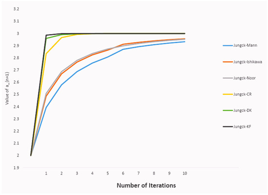
Figure 1. Comparison between Jungck-KF and other Jungck-type iterative schemes.

Table 2. Convergence of various Jungck-type iterative schemes to the coincidence point ${\underline{p}}^{*}=9=\zeta 3=\xi 3,$ with $a_0=2$ and ${\eta }_n={\sigma }_n={\displaystyle \frac{1}{\sqrt{2n+1}}}$.

n	Jungck-CR	Jungck-DK	Jungck-KF
	Iterative Scheme	Iterative Scheme	Iterative Scheme
	$\mathsf{\zeta }{\mathit{a}}_{\mathit{n}}$        $\mathsf{\xi }{\mathit{a}}_{\mathit{n}}$       ${\mathit{a}}_{\mathit{n}+\mathbf{1}}$	$\mathsf{\zeta }{\mathit{a}}_{\mathit{n}}$        $\mathsf{\xi }{\mathit{a}}_{\mathit{n}}$        ${\mathit{a}}_{\mathit{n}+\mathbf{1}}$	$\mathsf{\zeta }{\mathit{a}}_{\mathit{n}}$        $\mathsf{\xi }{\mathit{a}}_{\mathit{n}}$       ${\mathit{a}}_{\mathit{n}+\mathbf{1}}$
0	7.00000 4.00000 2.83474	7.00000 4.00000 2.95956	7.00000 4.00000 2.98649
1	8.66949 8.03578 2.96628	8.91912 8.75900 2.99051	8.97298 8.91912 2.99882
2	8.93255 8.79879 2.99238	8.98102 8.94315 2.99740	8.99854 8.99382 2.99997
3	8.98476 8.95435 2.99817	8.99480 8.98441 2.99924	8.99994 8.99982 2.99999
4	8.99634 8.98903 2.99954	8.99848 8.99544 2.99976	8.99998 8.99995 3.00000
5	8.99908 8.99725 2.99988	8.99952 8.99856 2.99993	8.99998 8.99995 3.00000
6	8.99976 8.99929 2.99997	8.99986 8.99958 2.99998	8.99998 8.99995 3.00000
7	8.99994 8.99981 2.99999	8.99996 8.99988 3.00000	8.99998 8.99995 3.00000
8	8.99998 8.99995 3.00000	8.99998 8.99998 3.00000	8.99998 8.99995 3.00000
9	9.00000 8.99999 3.00000	9.00000 9.00000 3.00000	8.99998 8.99995 3.00000
10	9.00000 9.00000 3.00000	9.00000 9.00000 3.00000	8.99998 8.99995 3.00000

5. Application in Dynamic Market Equilibrium

This section is dedicated to the analysis of Dynamic Market Equilibrium with respect to the common fixed-point result given in this paper. The role of coincident points and the Jungck sequence in the context of Dynamic Market Equilibrium was first studied by S. Shukla et. al. [32]. Then, starting with this work, we present an application to prove the practical utility of the Jungck contraction in determining the unique solution of an integral equation arising in the context of Dynamic Market Equilibrium in economics.

The concept of Dynamic Market Equilibrium lies at the intersection of economics and mathematics, particularly in economic dynamics, game theory, and mathematical optimization. It extends the classical notion of market equilibrium to systems that evolve over time, capturing how agents interact, adjust their behavior, and respond to changing market conditions.

Symmetry in an economic context may also refer to agent symmetry—where all agents are treated identically in terms of access to markets or preferences; preference symmetry—where agents have similar (e.g., homothetic or convex) preferences; or time symmetry—where future and past are treated analogously in intertemporal models.

While these are not mathematical symmetries of a norm, they influence whether the aggregated excess demand functions have properties (e.g., continuity, monotonicity, or convexity) that can be translated into functional–analytic terms for fixed-point theorems or variational inequality frameworks.

Supply ${\mathbf{M}}_s$ and demand ${\mathbf{M}}_d$ in many markets are influenced by current prices and price trends, including whether prices are rising or falling and the rate at which these changes occur (i.e., accelerating or decelerating) [33]. Consequently, an economist must consider the current price $\mathcal{P}\left(t\right)$, its first derivative ${\displaystyle \frac{d\mathcal{P}\left(t\right)}{dt}}$, and its second derivative ${\displaystyle \frac{d^2\mathcal{P}\left(t\right)}{d{t}^2}}$. Let

$$\begin{array}{cc}\hfill {\mathbf{M}}_s=& g_1+u_1\mathcal{P}\left(t\right)+e_1{\displaystyle \frac{d\mathcal{P}\left(t\right)}{dt}}+c_1{\displaystyle \frac{d^2\mathcal{P}\left(t\right)}{d{t}^2}}\hfill \\ \hfill {\mathbf{M}}_d=& g_2+u_2\mathcal{P}\left(t\right)+e_2{\displaystyle \frac{d\mathcal{P}\left(t\right)}{dt}}+c_2{\displaystyle \frac{d^2\mathcal{P}\left(t\right)}{d{t}^2}}\hfill \end{array}$$

where $g_1,g_2,u_1,u_2,e_1$, and $e_2$ are constants, and $c_1$ and $c_2$ are chosen such that $c_1-c_2\ne 0$. Equilibrium is given by ${\mathbf{M}}_s={\mathbf{M}}_d$. Therefore,

$$g_1+u_1\mathcal{P}\left(t\right)+e_1{\displaystyle \frac{d\mathcal{P}\left(t\right)}{dt}}+c_1{\displaystyle \frac{d^2\mathcal{P}\left(t\right)}{d{t}^2}}=g_2+u_2\mathcal{P}\left(t\right)+e_2{\displaystyle \frac{d\mathcal{P}\left(t\right)}{dt}}+c_2{\displaystyle \frac{d^2\mathcal{P}\left(t\right)}{d{t}^2}}$$

since

$$(c_1-c_2){\displaystyle \frac{d^2\mathcal{P}\left(t\right)}{d{t}^2}}+(e_1-e_2){\displaystyle \frac{d\mathcal{P}\left(t\right)}{dt}}+(u_1-u_2)\mathcal{P}\left(t\right)=-(g_1-g_2).$$

Letting $c=c_1-c_2$, $e=e_1-e_2,$$u=u_1-u_2$, and $g=g_1-g_2$ in the above, we have

$$c{\displaystyle \frac{d^2\mathcal{P}\left(t\right)}{d{t}^2}}+e{\displaystyle \frac{d\mathcal{P}\left(t\right)}{dt}}+u\mathcal{P}\left(t\right)=-g,$$

and dividing $\mathcal{P}\left(t\right)$ by $c\ne 0$ we get the following initial value problem:

$$\left\{\begin{array}{c}{\mathcal{P}}^{\prime \prime }+{\displaystyle \frac{e}{c}}{\mathcal{P}}^{\prime }+{\displaystyle \frac{u}{c}}\mathcal{P}\left(t\right)={\displaystyle \frac{-g}{c}};\hfill \\ \mathcal{P}\left(0\right)=0;\hfill \\ {\mathcal{P}}^{\prime }\left(0\right)=0.\hfill \end{array}\right.$$

(35)

Further, let $\mathcal{C}\left([0,\sigma ],\mathbb{R}\right)$ be the set of real continuous functions defined on $[0,\sigma ]$, with $\sigma >0$. Following the proof, it is easy to show that Problem (35) is equivalent to the integral equation

$$\begin{array}{c}\hfill \mathcal{P}\left(t\right)={\int }_0^{\sigma }\mathfrak{G}(t,v)\mathfrak{K}(t,v,\mathcal{P}\left(v\right))dv,\end{array}$$

(36)

where $\mathfrak{G}(t,v):[0,\sigma ]\times [0,\sigma ]\to [0,\sigma ]$ is a Green function defined as

$$\begin{array}{c}\hfill \mathfrak{G}(t,v)=\left\{\begin{array}{c}v·e^{{\displaystyle \frac{u}{2e}}(t-v)},\mathrm{if}0\le v\le t\le \sigma \hfill \\ t·e^{{\displaystyle \frac{u}{2e}}(v-t)},\mathrm{if}0\le t\le v\le \sigma \hfill \end{array}\right.\end{array}$$

(37)

and $\mathfrak{K}:[0,\sigma ]\times [0,\sigma ]\times C\left(\right[0,\sigma ],\mathbb{R})\to \mathbb{R}$ is a continuous and non-decreasing function.

Further, let us consider the following equation system:

$$\begin{array}{c}\hfill \left\{\begin{array}{c}{\mathcal{P}}_1\underline{x}\left(t\right)={\int }_0^{\sigma }\mathfrak{G}(t,v)\mathfrak{K}(t,v,{\mathcal{P}}_1\underline{x}\left(v\right))dv\hfill \\ {\mathcal{P}}_2\underline{y}\left(t\right)={\int }_0^{\sigma }\mathfrak{G}(t,v)\mathfrak{H}(t,v,{\mathcal{P}}_2\underline{y}\left(v\right))dv.\hfill \end{array}\right.\end{array}$$

(38)

where $\mathfrak{K},\mathfrak{H}:[0,\sigma ]\times [0,\sigma ]\times C[0,\sigma ]\to \mathbb{R}$ are two continuous and non-decreasing functions and $\mathfrak{G}(t,v)$ is a Green function defined as (37).

Let ${\parallel .\parallel }_{\infty }:X\times X\to \mathbb{R}$ be a norm defined by

$$\begin{array}{c}\hfill {\parallel \zeta a-\zeta b\parallel }_{\infty }=\underset{t\in [0,\sigma ]}{sup}|\zeta a-\zeta b|,\mathrm{for}a,b\in \mathbb{R}.\end{array}$$

(39)

It is easy to prove that $X=\left(C\left([0,\sigma ],\mathbb{R}\right),{\parallel .\parallel }_{\infty }\right)$ form a Banach space.

Theorem 5.

Let $X=\left({C([0,\sigma ],\mathbb{R}),\parallel .\parallel }_{\infty }\right)$ be a Banach space. Assume Equation (36) holds and that the following assertions are true:

(i) 

There exists an arbitrary subset A of X and $\xi ,\zeta :A\to X$, two weakly compatible mappings with the same properties as in Theorem 1, such that for $\underline{x}\left(t\right),\underline{y}\left(t\right)\in X$ we have

$$\begin{array}{cc}\hfill \zeta \underline{x}\left(t\right)=& {\int }_0^{\sigma }\mathfrak{G}(t,v)\mathfrak{K}(t,v,\zeta \underline{x}\left(v\right))dv;\hfill \end{array}$$

(40)

$$\begin{array}{cc}\hfill \xi \underline{y}\left(t\right)=& {\int }_0^{\sigma }\mathfrak{G}(t,v)\mathfrak{H}(t,v,\xi \underline{y}\left(v\right))dv,\hfill \end{array}$$

(41)

where $\mathfrak{K},\mathfrak{H}:[0,\sigma ]\times C[0,\sigma ]\to \mathbb{R}$ are two continuous and non-decreasing functions and $\mathfrak{G}(t,v):[0,\sigma ]\times [0,\sigma ]\to [0,\sigma ]$ is a Green function defined in (37) that is continuous and bounded as follows:

$$\underset{t\in [0,\sigma ]}{sup}{\int }_0^{\sigma }\left|\mathfrak{G}(t,v)\right|\le 1;$$

(ii) 

There exists a monotone increasing function $\upsilon :{\mathbb{R}}^{+}\to {\mathbb{R}}^{+}$ with the property $\upsilon \left(0\right)=0$ and $\widehat{r}\in [0,1]$ such that

$$|\mathfrak{K}(t,v,\zeta \left(a\right))-\mathfrak{H}(t,v,\zeta \left(b\right))|\le |\upsilon (\xi a-\zeta b)+\widehat{r}(\xi a-\xi b)|,\mathrm{for}\sigma >0\mathrm{and}a,b\in \mathbb{R}.$$

Then, the integral equation system (38) has a unique common solution.

Proof. 

In order to prove this Theorem, we will check the Jungck-KF condition (5) for every $\underline{x}\left(t\right),\underline{y}\left(t\right)\in C[0,\sigma ]$.

$$\begin{array}{cc}\hfill |\zeta \underline{x}\left(t\right)-\zeta \underline{y}\left(t\right)|=& \left|{\int }_0^{\sigma }\mathfrak{G}(t,v)\mathfrak{K}(t,v,\zeta \underline{x}\left(v\right))dv-{\int }_0^{\sigma }\mathfrak{G}(t,v)\mathfrak{H}(t,v,\zeta \underline{y}\left(v\right))dv\right|\hfill \\ \hfill \le & {\int }_0^{\sigma }\left|\mathfrak{G}(t,v)\right|·|\mathfrak{K}(t,v,\zeta \underline{x}\left(v\right))-\mathfrak{H}(t,v,\zeta \underline{y}\left(v\right))|dv.\hfill \end{array}$$

Using the assumption $\left(ii\right)$ we have

$$\begin{array}{cc}\hfill |\zeta \underline{x}\left(t\right)-\zeta \underline{y}\left(t\right)|& \le {\int }_0^{\sigma }\left|\mathfrak{G}(t,v)\right|·\left|\upsilon (\xi \underline{x}\left(v\right)-\zeta \underline{y}\left(v\right))+\widehat{r}(\xi \underline{x}\left(v\right)-\xi \underline{y}\left(v\right))\right|dv.\hfill \end{array}$$

Taking the supremum on both sides, and taking into account that $\upsilon :{\mathbb{R}}^{+}\to {\mathbb{R}}^{+}$ is a monotone increasing function, for $\widehat{r}\in [0,1]$, we get

$$\begin{array}{cc}\hfill & \underset{t\in [0,\sigma ]}{sup}|\zeta \underline{x}\left(t\right)-\zeta \underline{y}\left(t\right)|\le \underset{t\in [0,\sigma ]}{sup}\left({\int }_0^{\sigma }\left|\mathfrak{G}(t,v)\right|·\left|\upsilon (\xi \underline{x}\left(v\right)-\zeta \underline{y}\left(v\right))+\widehat{r}(\xi \underline{x}\left(v\right)-\xi \underline{y}\left(v\right))\right|dv\right)\hfill \\ \hfill & \le {\int }_0^{\sigma }\underset{t\in [0,\sigma ]}{sup}\left|\mathfrak{G}(t,v)\right|·\underset{t\in [0,\sigma ]}{sup}\left|\upsilon (\xi \underline{x}\left(v\right)-\zeta \underline{y}\left(v\right))+\widehat{r}(\xi \underline{x}\left(v\right)-\xi \underline{y}\left(v\right))\right|dv\hfill \\ \hfill & \le {\int }_0^{\sigma }\underset{t\in [0,\sigma ]}{sup}\left|\mathfrak{G}(t,v)\right|·\left[\underset{t\in [0,\sigma ]}{sup}\left|\upsilon (\xi \underline{x}\left(v\right)-\zeta \underline{y}\left(v\right))\right|+\widehat{r}\underset{t\in [0,\sigma ]}{sup}\left|\xi \underline{x}\left(v\right)-\xi \underline{y}\left(v\right)\right|\right]dv\hfill \\ \hfill & \le {\int }_0^{\sigma }\underset{t\in [0,\sigma ]}{sup}\left|\mathfrak{G}(t,v)\right|·\left[\upsilon \left(\underset{t\in [0,\sigma ]}{sup}\left|\xi \underline{x}\left(v\right)-\zeta \underline{y}\left(v\right)\right|\right)+\widehat{r}\underset{t\in [0,\sigma ]}{sup}\left|\xi \underline{x}\left(v\right)-\xi \underline{y}\left(v\right)\right|\right]dv.\hfill \end{array}$$

Then we have

$$\parallel \zeta \underline{x}-\zeta \underline{y}{\parallel }_{\infty }\le \left[\upsilon (\parallel \xi \underline{x}-\zeta \underline{y}{\parallel }_{\infty })+\widehat{r}{\parallel \xi \underline{x}-\xi \underline{y}\parallel }_{\infty }\right]{\int }_0^{\sigma }\underset{t\in [0,\sigma ]}{sup}\left|\mathfrak{G}(t,v)\right|dv.$$

Since the Green function is bounded as in $\left(ii\right)$, we get

$$\parallel \zeta \underline{x}-\zeta \underline{y}{\parallel }_{\infty }\le \upsilon (\parallel \xi \underline{x}-\zeta \underline{x}{\parallel }_{\infty })+\widehat{r}{\parallel \xi \underline{x}-\xi \underline{y}\parallel }_{\infty }$$

Then, the Jungck contraction condition given in (5) holds. Applying Theorem 1, for ${\mathcal{P}}_1\underline{x}=\zeta \underline{x}$ and ${\mathcal{P}}_2\underline{y}=\xi \underline{y}$, we get the existence of a unique common solution of the integral equation system (38)—$x^{*}\in \mathcal{C}[0,\sigma ]$—which is derived from the price equation (36). Meanwhile, considering that the economic problem of determining market equilibrium is seen as a boundary value problem (35), the common unique solution of the integral equation system (38) is actually the equilibrium price of the market. □

6. Conclusions

The Jungck-KF iterative scheme’s efficiency stems from its comprehensive contractive conditions, enhanced stability and data-dependence, superior convergence rates, and flexibility in operator pairing. These attributes make it a robust choice for researchers and practitioners working within fixed-point theory and related fields. Also, the implications of the data-dependence result for the Jungck-KF iterative scheme are profound, enhancing its robustness, accuracy, applicability, efficiency, and potential for algorithmic innovation. These factors collectively contribute to its growing relevance in practical applications across diverse fields.

We also explored an application to prove the practical utility of the Jungck contraction in determining the unique solution of an integral equation arising in the context of dynamic market equilibrium in economics.

Also, a strong connection between norm symmetry in Banach spaces and dynamic market equilibrium models was made evident in this study. At a foundational level, norm symmetry ensures basic mathematical consistency in equilibrium formulations. Also, geometric symmetries in Banach spaces underpin the existence, uniqueness, and convergence of equilibrium in dynamic settings. These symmetries enable the use of fixed-point theory and variational analysis, which are central to proving results in dynamic general equilibrium theory and computational economics.

References

- Ostrowski, A.M. Solution of Equations and Systems of Equation; Academic Press: New York, NY, USA, 1960; Volume IX. [Google Scholar]
- Petković, M.S.; Neta, B.; Petković, L.; Džunić, J. Multipoint Methods for Solving Nonlinear Equation; Elsevier: Amsterdam, The Netherlands, 2013. [Google Scholar]
- Bnouhachem, A.; Noor, M.A. A new iterative method for variational inequalities. Appl. Math. Comput. 2006, 182, 1673–1682. [Google Scholar] [CrossRef]
- Noor, M.A.; Noor, K.I.; Bnouhachem, A. Some new iterative methods for solving variational inequalities. Can. J. Appl. Math. 2020, 2, 1–17. [Google Scholar]
- Ceng, L.-C.; Al-Homidan, S.; Ansari, Q.H.; Yao, J.-C. An iterative scheme for equilibrium problems and fixed point problem of strict-pseudo-contraction mappings. J. Comput. Appl. Math. 2009, 223, 967–974. [Google Scholar] [CrossRef]
- Ceng, L.-C.; Petrusel, A.; Yao, J.-C. Iterative approaches to solving equilibrium problems and fixed point problems of infinitely many nonexpansive mappings. J. Optim. Theory Appl. 2009, 143, 37–58. [Google Scholar] [CrossRef]
- Jia, J.; Shabbir, K.; Ahmad, K.; Shah, N.A.; Botmart, T. Strong convergence of a new hybrid iterative scheme for nonexpensive mappings and applications. J. Funct. Spaces 2022, 1, 4855173. [Google Scholar]
- Chugh, R.; Kumar, V. Data dependence of Noor and SP iterative schemes when dealing with quasi-contractive operators. Int. J. Comput. Appl. 2011, 36, 40–46. [Google Scholar] [CrossRef]
- Qing, Y.; Rhoades, B.E. Comments on the rate of convergence between Mann and Ishikawa iterations applied to Zamfirescu operators. Fixed Point Theory Appl. 2008, 2008, 387504. [Google Scholar] [CrossRef]
- Banach, S. Sur les opérations dans les ensembles abstraits et leur application aux équations intégrales. Fundam. Math. 1922, 3, 133–181. [Google Scholar] [CrossRef]
- Abbas, M.; Jungck, G. Common fixed point results for noncommuting mappings without continuity in cone metric spaces. J. Math. Anal. Appl. 2008, 341, 416–420. [Google Scholar] [CrossRef]
- Bouhadjera, H. A unique common fixed point for contractive mappings under a new concept. Bull. Transilv. Univ. Brasov. Ser. III Math. Comput. Sci. 2022, 2, 33–46. [Google Scholar] [CrossRef]
- Kumar, S.; Aron, D. Common fixed-point theorems for non-linear non-self contractive mappings in convex metric spaces. Topol. Algebra Its Appl. 2023, 11, 20220122. [Google Scholar] [CrossRef]
- Chandok, S.; Radenović, S. Existence of solution for orthogonal F-contraction mappings via Picard–Jungck sequences. J. Anal. 2022, 30, 677–690. [Google Scholar] [CrossRef]
- Fan, H.; Wang, C. Stability and convergence rate of Jungck-type iterations for a pair of strongly demicontractive mappings in Hilbert spaces. Comput. Appl. Math. 2023, 14, 33. [Google Scholar] [CrossRef]
- Maldar, S. An examination of data dependence for Jungck-Type iteration method. Erciyes Üniv. Fen Bilim. Enstitüsü Fen Bilim. Derg. 2020, 36, 374–384. [Google Scholar]
- Jamil, Z.Z.; Hussein, Z. Common Fixed Point of Jungck Picard Itrative for Two Weakly Compatible Self-Mappings. Iraqi J. Sci. 2021, 62, 1695–1701. [Google Scholar]
- Bosede, A.O. Strong convergence results for the Jungck-Ishikawa and Jungck-Mann iteration processes. Bull. Math. Anal. Appl. 2010, 2, 65–73. [Google Scholar]
- Berinde, V. On the convergence of the Ishikawa iteration in the class of quasi contractive operators. Acta Math. Univ. Comen. New Ser. 2004, 73, 119–126. [Google Scholar]
- Berinde, V.; Takens, F. Iterative Approximation of Fixed Points; Springer: Berlin/Heidelberg, Germany, 2007; Volume 1912. [Google Scholar]
- Guran, L.; Shabbir, K.; Ahmad, K.; Bota, M.F. Stability, Data Dependence, and Convergence Results with Computational Engendering of Fractals via Jungck-DK Iterative Scheme. Fractal Fract. 2023, 7, 418. [Google Scholar] [CrossRef]
- Harder, A.M. Fixed Point Theory and Stability Results for Fixed Point Iteration Procedures. 1987. Doctoral Dissertations. 634. Available online: https://scholarsmine.mst.edu/doctoral_dissertations/634 (accessed on 27 April 2025).
- Hussain, N.; Kumar, V.; Kutbi, M.A. On rate of convergence of Jungck-type iterative schemes. Abstr. Appl. Anal. 2013, 2013, 132626. [Google Scholar] [CrossRef]
- Jungck, G. Commuting mappings and fixed points. Am. Math. Mon. 1976, 83, 261–263. [Google Scholar] [CrossRef]
- Ostrowski, A.M. The Round-off Stability of Iterations. ZAMM-J. Appl. Math. Mech./Z. Angew. Math. Mech. 1967, 47, 77–81. [Google Scholar] [CrossRef]
- Olatinwo, M.O.; Imoru, C.O. Some convergence results for the Jungck–Mann and the Jungck–Ishikawa iteration processes in the class of generalized Zamfirescu operators. Acta Math. Univ. Comen. New Ser. 2008, 27, 299–304. [Google Scholar]
- Singh, S.L.; Bhatnagar, C.; Mishra, S.N. Stability of Jungck-type iterative procedures. Int. J. Math. Math. Sci. 2005, 2005, 3035–3043. [Google Scholar] [CrossRef]
- Olatinwo, M.O. A generalization of some convergence results using the Jungck-Noor three step iteration process in arbitrary Banach space. Fasc. Math. 2008, 40, 37–43. [Google Scholar]
- Ullah, K.; Ahmad, J.; Khan, F.M. Numerical reckoning fixed points via new faster iteration process. Appl. Gen. Topol. 2022, 23, 213–223. [Google Scholar] [CrossRef]
- Jungck, G.; Hussain, N. Compatible maps and invariant approximations. J. Math. Anal. Appl. 2007, 325, 1003–1012. [Google Scholar] [CrossRef]
- Soltuz, S.M.; Grosan, T. Data dependence for Ishikawa iteration when dealing with contractive-like operators. Fixed Point Theory Appl. 2008, 2008, 242916. [Google Scholar] [CrossRef]
- Shukla, S.; Dubey, N.; Shukla, R.; Mezník, I. Coincidence Point of Edelstein Type Mappings in Fuzzy Metric Spaces and Application to the Stability of Dynamic Markets. Axioms 2023, 12, 854. [Google Scholar] [CrossRef]
- Dowling Edward, T. Introduction to Mathematical Economics; MC Graw Hill Education: New York, NY, USA, 2001. [Google Scholar]
Disclaimer/Publisher’s Note: The statements, opinions and data contained in all publications are solely those of the individual author(s) and contributor(s) and not of MDPI and/or the editor(s). MDPI and/or the editor(s) disclaim responsibility for any injury to people or property resulting from any ideas, methods, instructions or products referred to in the content. |
© 2025 by the authors. Licensee MDPI, Basel, Switzerland. This article is an open access article distributed under the terms and conditions of the Creative Commons Attribution (CC BY) license (https://creativecommons.org/licenses/by/4.0/).