A Novel Symmetrical Inertial Alternating Direction Method of Multipliers with Proximal Term for Nonconvex Optimization with Applications

Abstract

In this paper, we propose a novel alternating direction method of multipliers based on acceleration technique involving two symmetrical inertial terms for a class of nonconvex optimization problems with a two-block structure. To address the nonconvex subproblem, we introduce a proximal term to reduce the difficulty of solving this subproblem. For the smooth subproblem, we employ a gradient descent method on the augmented Lagrangian function, which significantly reduces the computational complexity. Under appropriate assumptions, we prove subsequential convergence of the algorithm. Moreover, when the generated sequence is bounded and the auxiliary function satisfies Kurdyka–Łojasiewicz property, we establish global convergence of the algorithm. Finally, effectiveness and superior performance of the proposed algorithm are validated through numerical experiments in signal processing and smoothly clipped absolute deviation penalty problems.

1. Introduction

It is well known that recovering sparse signals from incomplete observations is an important and very significant research topic in practical applications. The core objective is to find the optimal sparse solution to a system of linear equations, which can be formulated as the following model [1]:

$$minc{\parallel x\parallel }_0+{\displaystyle \frac{1}{2}}\parallel Ax-b\parallel ,$$

(1)

where $A\in {\mathbb{R}}^{m\times n}$ is the measurement matrix, $b\in {\mathbb{R}}^m$ is the observed data, $x\in {\mathbb{R}}^n$ is a sparse signal, $c>0$ is a regularization parameter, and ${\parallel ·\parallel }_0$ denotes the ${\ell }_0$-norm. However, Chartrand and Staneva [2] pointed out that (1) represents a class of problems that are fundamentally difficult to solve. To overcome this challenge, Zeng et al. [3] proposed a relaxed objective function by replacing the $l_0$ regularization with the $l_{\frac{1}{2}}$ regularization; the model (1) is transformed into a more tractable nonconvex optimization problem. Therefore, adopting this modification becomes more reasonable in signal recovery problems, which leads to the following two-block nonconvex optimization problem:

$$\begin{array}{c}\hfill minc{\parallel x\parallel }_{\frac{1}{2}}^{\frac{1}{2}}+\frac{1}{2}{\parallel Ax-b\parallel }^2,\end{array}$$

(2)

where ${\parallel x\parallel }_{\frac{1}{2}}^{\frac{1}{2}}={\sum }_{i=1}^n{\left|x_i\right|}^{\frac{1}{2}}$. Further, to mitigate feature compression and information loss in motor imagery decoding, Doostmohammadian et al. [4] proposed a Cauchy-based nonconvex sparse regularization model, which enhances feature extraction and noise reduction across datasets. In general, introducing an auxiliary variable $z\in {\mathbb{R}}^m$ such that $z=Ax-b$ in (2), we would consider reformulating the problem (2) as follows:

$$\begin{array}{c}minc{\parallel x\parallel }_{\frac{1}{2}}^{\frac{1}{2}}+\frac{1}{2}{\parallel z\parallel }^2\\ \mathrm{s}.\mathrm{t}. Ax-z=b.\end{array}$$

(3)

We notice that many scholars have investigated constrained nonconvex optimization problems of the form (3). In particular, Zeng et al. [3] pointed out that the iterative soft-thresholding algorithm can be used to solve the regularization problem, which was validated in the context of problem (3). Meanwhile, Chen and Selesnick [5] performed a performance validation of model (3) using an improved overlapping shrinkage algorithm. Further related works can be found in [6,7] and the references therein.

In order to solve (3), we will consider the general model of (3) in this paper. That is, in (3), extending the objective function, respectively, to a lower semicontinuous function $f:{\mathbb{R}}^n\to \mathbb{R}$ and a differentiable function $g:{\mathbb{R}}^m\to \mathbb{R}$ whose gradient is L-Lipschitz continuous with $L>0$, and setting ${\mathbb{R}}^m\ni y=-z$, the problem (3) is generalized as the following nonconvex optimization with linear constraints:

$$\begin{array}{c}min f\left(x\right)+g\left(y\right)\\ \mathrm{s}.\mathrm{t}. Ax+y=b,\end{array}$$

(4)

where A is the same as in (1). In recent years, nonconvex optimization problems of the form (4) have found widespread applications in science and engineering. For instance, based on a gradient tracking algorithm, Zhang et al. [8] investigated optimization of local nonconvex objective functions in time-varying networks. In addition, to ensure the effectiveness of image reconstruction, Tiddeman and Ghahremani [9] combined wavelet transforms with principal component analysis to propose a class of principal component waveform networks for solving linear inverse problems, and fully utilized the symmetry in wavelet transforms during the wavelet decomposition. For more related works, one can see [10,11,12] and the references therein.

In fact, variants of (4) have found applications in various fields, such as statistical learning [13,14,15], penalized zero-variance discriminant analysis [16] and image reconstruction [17,18]. Furthermore, if $y=-p$, $f\left(x\right)={\sum }_{i=1}^n{h}_k\left(\right|x_i\left|\right)$ for $x={(x_1,x_2,\cdots ,x_n)}^T\in {\mathbb{R}}^n$ and $g\left(y\right)={\displaystyle \frac{1}{2}}{\parallel y\parallel }^2={\displaystyle \frac{1}{2}}{\parallel p\parallel }^2$ in (4), then the nonconvex optimization degenerates to the following smoothly clipped absolute deviation (SCAD) penalty problem:

$$\begin{array}{c}min \sum _{i=1}^n{h}_k\left(\right|x_i\left|\right)+{\displaystyle \frac{1}{2}}{\parallel p\parallel }^2\\ \mathrm{s}.\mathrm{t}. Ax-p=b,\end{array}$$

(5)

with the penalty function $h_{\kappa }$ in the objective, we refer readers to (26) later. The SCAD penalty problem (5) proposed by scholars can be conceptually understood and it should be noted that in statistical optimization, certain penalty methods exhibit limitations, such as vulnerability to data circumvention and biased estimation of significant variables [19]. To address these questions, Fan and Li [20] proposed a SCAD penalty function, developed optimization algorithms to solve nonconcave penalized likelihood problems and demonstrated that this method possesses asymptotic oracle properties. Remarkably, with appropriate regularization parameter selection, the results can achieve nearly identical performance to the known true model.

It is well known that alternating direction method of multipliers (ADMM) has gained widespread attention due to its balance between performance and efficiency. When the subproblems are independent, ADMM exhibits a unique symmetry. In fact, with appropriately designed update steps, this symmetry ensures that the convergence of ADMM is independent of the order in which the subproblems are updated [21]. In recent years, as nonconvex optimization problems have gained increasing attention, convergence analysis of ADMM in nonconvex settings has become a research hotspot. Due to the lack of theoretical guarantees for ADMM in nonconvex problems, Hong et al. [22] not only established a convergence theory for ADMM in the nonconvex setting, but also overcame the limitation on the number of variable blocks. Wang et al. [23] demonstrated that incorporating the Bregman distance into ADMM can effectively simplify the computation of subproblems, emphasizing the feasibility of ADMM in nonconvex settings. Ding et al. [24] proposed a class of semi-proximal ADMM for solving low-rank matrix recovery problems. Furthermore, in the presence of noisy matrix data, by minimizing the nuclear norm, Ding et al. [24] effectively addressed the issues of Gaussian noise and related mixed noise. Guo et al. [25] provided insights into solving large-scale nonconvex optimization problems using ADMM. For more related work, readers may refer to [26,27,28,29] and the references therein.

The inertial acceleration technique, which is derived from the heavy-ball method, utilizes information from previous iterations to construct affine combinations [30]. Additionally, we observe that the inertial technique can employ different extrapolation strategies during the optimization process to enhance convergence speed. Using a general inertial proximal gradient method, Wu and Li [31] proposed two distinct extrapolation strategies to flexibly adjust convergence rate of the inertial proximal gradient method. Chao et al. [32] investigated an inertial proximal ADMM and established the global convergence of iterates under appropriate assumptions. Moreover, Wang et al. [33] considered a different inertial update scheme, which not only preserves the acceleration effect of inertia but also reduces the computational error caused by the inertial term.

Unfortunately, Wang et al. [33] only considered the inertial update step for x. We note that Chen et al. [34] also discovered that embedding the inertial term into the y-subproblem can significantly improve convergence speed of the presented algorithm. Inspired by the work in [33,34], we adopt the inertial update step for x proposed by Wang et al. [33], and additionally consider an inertial update step for y to further accelerate the convergence of the algorithm. Based on this, we propose a novel symmetrical inertial alternating direction method of multipliers with proximal term (NIP-ADMM) to solve (4) and two application problems (3) and (5). Our main contributions can be summarized as follows:

(i)

Building upon the inertial update step due to [33], we introduce an additional inertial update for y and incorporate ${\overline{y}}^k$ into the x-subproblem update; this form of inertial update ensures that the primal variables are treated equally, and thereby we achieve faster acceleration. In addition, we introduce two distinct inertial parameters to avoid the differentiated feedback effect that a single inertial parameter may impose on different inertial terms.

(ii)

To simplify the computation of the subproblems, we introduce an approximation term in the x-subproblem, which under appropriate conditions, a closed-form solution can be obtained in practical applications.

(iii)

Under reasonable assumptions, we prove that any cluster point of the sequence generated by NIP-ADMM belongs to the set of critical points of the augmented Lagrangian function. Furthermore, under the condition that the auxiliary function satisfies Kurdyka–Łojasiewicz property (KLP), we further establish that the sequence generated by NIP-ADMM converges to a stationary point of the augmented Lagrangian function.

(iv)

Since function g in (4) is convex, this ensures that g is well-defined, and enables us to abandon the traditional ADMM update scheme and instead adopt a gradient descent approach. This method requires only the computation of gradients at each iteration, and significantly reduces computational complexity. Consequently, it offers substantial advantages when handling high-dimensional or large-scale datasets.

The structure of this paper is as follows. In Section 2, we review essential results required for further analysis. We present NIP-ADMM and analyze its convergence in Section 3. Numerical experiment and application to signal recovery model and SCAD penalty problem in Section 4 highlight the benefits of the majorization and inertial techniques. Lastly, in Section 5, we provide a conclusion.

2. Preliminaries

In this section, we introduce key notations and definitions that are essential for the results to be developed and are utilized in the subsequent sections.

Assume $\langle x,y\rangle =x^{T}y$ and $\parallel x\parallel =\sqrt{\langle x,x\rangle }$ for $x,y\in {\mathbb{R}}^n$. If matrix S is a positive definite (semi-definite positive) matrix, then we have $S\succ 0 (S⪰0)$. Given any $n\times n$ matrix $S⪰0$ and a vector $x\in {\mathbb{R}}^n$, let ${\parallel x\parallel }_S:=\sqrt{x^{T}Sx}$ be S-norm of x. For a matrix $D\in {\mathbb{R}}^{n\times m}$, we define ${\lambda }_{{min}_{\left(D\right)}}$ and ${\lambda }_{{max}_{\left(D\right)}}$ as the smallest and largest eigenvalues of $D^{T}D$, respectively. If we denote $f:{\mathbb{R}}^n\to (-\infty ,+\infty ]$, then the domain of f is defined as $dom f=\{x\in {\mathbb{R}}^n|f\left(x\right)<+\infty \}$.

Definition 1.

Let $Q\subseteq {\mathbb{R}}^n$. Then the distance from point $x\in {\mathbb{R}}^n$ to Q is defined as $d(x,Q)={inf}_{y\in Q}\parallel y-x\parallel$. In particular, if $Q=\varnothing$, then $d(x,Q)=+\infty$.

Definition 2.

For a differentiable convex function $F:{\mathbb{R}}^n\to \mathbb{R}$, Bregman distance is defined by

$${▵}_F(p,q)=F\left(p\right)-F\left(q\right)-\langle \nabla F\left(q\right),p-q\rangle ,\hspace{1em}\forall p,q\in {\mathbb{R}}^n.$$

Definition 3.

Assume $\chi :{\mathbb{R}}^n\to \mathbb{R}\cup \{+\infty \}$ is a proper lower semicontinuous function.

(i)

Frechet sub-differential of χ at $x\in \mathrm{dom}\chi$ is denoted by $\widehat{\partial }\chi \left(x\right)$ and defined as:

$$\widehat{\partial }\chi \left(x\right)=\left\{\overline{x}\in {\mathbb{R}}^n:\underset{y\ne x}{lim}\underset{y\to x}{inf}{\displaystyle \frac{\chi \left(y\right)-\chi \left(x\right)-〈\overline{x},y-x〉}{\parallel y-x\parallel }}\ge 0\right\}.$$

Among others, we set $\widehat{\partial }\chi \left(x\right)=\varnothing$ when $x\notin \mathrm{dom}\chi$.

(ii)

The limiting sub-differential of χ at $x\in \mathrm{dom}\chi$ is written as $\partial \chi \left(x\right)$ and defined by

$$\partial \chi \left(x\right)=\left\{\overline{x}\in {\mathbb{R}}^n:\exists x_k\to x,\chi \left(x_k\right)\to \chi \left(x\right),{\widehat{x}}_k\in \widehat{\partial }\chi \left(x_k\right),{\widehat{x}}_k\to \overline{x}\right\}.$$

Definition 4.

We say the point $(x^{★},y^{★},{\lambda }^{★})$ is a critical point of the following augmented Lagrangian function associated with problem (4):

$$\begin{array}{c}{L}_{\beta }(x,y,\lambda )=f\left(x\right)+g\left(y\right)-\langle \lambda ,Ax+y-b\rangle +{\displaystyle \frac{\beta }{2}}{\parallel Ax+y-b\parallel }^2,\end{array}$$

(6)

where λ denotes the augmented Lagrange multiplier, and $\beta >0$ is a penalty parameter, if it satisfies the following conditions:

$$\left\{\begin{array}{c}{A}^T{\lambda }^{★}\in \partial f\left(x^{★}\right),\hfill \\ {\lambda }^{★}=\nabla g\left(y^{★}\right),\hfill \\ A{x}^{★}+y^{★}=b.\hfill \end{array}\right.$$

Definition 5

([35]). (KLP) Let $\chi :{\mathbb{R}}^n\to \mathbb{R}\cup \{+\infty \}$ be a proper lower semicontinuous function with $\partial \chi \ne \varnothing$. For $\widehat{p}\in \partial \chi$, if there exists $\varsigma \in (0,+\infty )$, a neighborhood U of $\widehat{p}$, and a function $\phi \in V_{\phi }$, where $V_{\phi }$ is the set of the concave function $\phi :[0,\varsigma )\to [0,+\infty )$, then for any $p\in \{p\in U\mid \chi \left(\widehat{p}\right)<\chi \left(p\right)<\chi \left(\widehat{p}\right)+\varsigma \}$, the following inequality holds:

$${\phi }^{\prime }(\chi \left(p\right)-\chi \left(\widehat{p}\right))d(0,\partial \chi \left(p\right))\ge 1.$$

We say that χ has KLP at $\widehat{p}$, and φ is the associate function of f with KLP.

Lemma 1

([36]). The sub-differential of a lower semicontinuous function $\chi :{\mathbb{R}}^n\to \mathbb{R}\cup \{+\infty \}$ possesses several fundamental and significant properties as follows:

(i)

From Definition 3, which implies that $\widehat{\partial }\chi \left(x\right)\subseteq \partial \chi \left(x\right)$ holds for all $x\in {\mathbb{R}}^n$, and given that $\partial \chi \left(x\right)$ is a closed set, $\widehat{\partial }\chi \left(x\right)$ is also a closed set.

(ii)

Suppose that $(x^k,y^k)$ is a sequence that converges to $(x^{★},y^{★})$, and $\chi \left(x^k\right)$ converges to $\chi \left(x^{★}\right)$ with $y^k\in \partial \chi \left(x^k\right)$. Then, by the definition of the sub-differential, we have $y^{★}\in \partial \chi \left(x^{★}\right)$.

(iii)

If $x^{★}$ is a local minimum of χ, then it follows that $0\in \partial \chi \left(x^{★}\right)$.

(vi)

Assuming that $F:{\mathbb{R}}^n\to \mathbb{R}$ is a continuously differentiable function, we can derive:

$$\partial (\chi +F)\left(x\right)=\partial \chi \left(x\right)+\nabla F\left(x\right).$$

Lemma 2

([35]). Assume $\mathrm{Y}(x,y)=f\left(x\right)+g\left(y\right)$, where $f:{\mathbb{R}}^n\to \mathbb{R}\cup \{+\infty \}$ and $g:{\mathbb{R}}^m\to \mathbb{R}\cup \{+\infty \}$ are both proper lower semicontinuous functions. Then, for any $(x,y)\in \mathit{dom} \mathrm{Y}=\mathit{dom} f\times \mathit{dom} g$, we can obtain

$$\partial \mathrm{Y}(x,y)={\partial }_{x}f(x,y)\times {\partial }_{y}g(x,y).$$

Lemma 3

([37]). (Uniformized KLP) Let Ω be a compact set and $V_{\phi }$ be the same as in Definition 5. If a proper lower semicontinuous function $\chi :{\mathbb{R}}^n\to \mathbb{R}\cup \{+\infty \}$ is fixed at a point in Ω and satisfies the KLP at every point on Ω, and there exist $\varrho >0$, $\varsigma >0$, and $\phi \in V_{\phi }$ such that for any $\widehat{x}\in \Omega$ and $x\in \{x\in {\mathbb{R}}^n:d(x,\Omega )<\varrho \}\cap [\chi \left(\widehat{x}\right)<\chi \left(x\right)<\chi \left(\widehat{x}\right)+\varsigma ]$, then the following inequality is satisfied:

$${\phi }^{\prime }(\chi \left(x\right)-\chi \left(\widehat{x}\right))d(0,\partial \chi \left(x\right))\ge 1.$$

Lemma 4

([38]). If the function $c:{\mathbb{R}}^n\to \mathbb{R}$ is continuously differentiable, and $\nabla c$ is Lipschitz continuous with constant $L\ge 0$, then for any $x,y\in {\mathbb{R}}^n$, the following result holds:

$$|c\left(y\right)-c\left(x\right)-\langle \nabla c\left(x\right),y-x\rangle |\le {\displaystyle \frac{L}{2}}{\parallel y-x\parallel }^2.$$

3. Novel Algorithm and Convergence Analysis

In this section, based on (6), we propose NIP-ADMM for solving the problem (4), which is outlined below:

Algorithm 1 NIP-ADMM

Initialization: Input $x^1,y^1$, and ${\lambda }^1$, and let ${\overline{x}}^0=x^1$, and ${\overline{y}}^0=y^1$. Given constants $\eta ,\theta \in (0,1]$, $\gamma ,\beta \in (0,+\infty ]$ and $S\in {\mathbb{R}}^{n\times n}$. Set appropriate stopping parameters $\varpi \in \mathbb{R}$, choose a sufficiently small $\mathfrak{h}$, and finally set $k=1$. for k = 0, 1, 2, …do 1° Compute $({\overline{x}}^k,{\overline{y}}^k)=(x^k,y^k)+\theta (x^k-{\overline{x}}^{k-1},0)+\eta (0,y^k-{\overline{y}}^{k-1})$. 2° Execute $argmin\{L_{\beta }(x,{\overline{y}}^k,{\lambda }^k)+{\displaystyle \frac{1}{2}}\parallel x-{\overline{x}}^k{\parallel }_S^2$ to determine $x^{k+1}$. 3° Calculate $y^{k+1}=y^k-\gamma {\nabla }_y{L}_{\beta }(x^{k+1},y^k,{\lambda }^k)$. 4° Update dual variable ${\lambda }^{k+1}={\lambda }^k-\beta (A{x}^{k+1}+y^{k+1}-b)$. 5° If $\varpi \le \mathfrak{h}$ then  break else  $k=k+1$ and continue End for 6° Output: output $(x^{k+1},y^{k+1},{\lambda }^{k+1})$ of the problem (4).

Remark 1.

(i) In Algorithm 1, S is a semi-definite matrix. Moreover, the parameters ϖ appearing in $5^{\circ }$ could be related to $\parallel x^{k+1}-x^k\parallel$ and $\parallel y^{k+1}-y^k\parallel$.

(ii)

The update scheme in $3^{\circ }$ of Algorithm 1 for y-subproblem adopts the gradient descent method, where ${\nabla }_y{L}_{\beta }$ is the gradient of the function $L_{\beta }$ with respect to y, and γ is called the learning rate.

(iii)

The inertial structure adopted in Algorithm 1 employs a structurally balanced acceleration strategy. This update strategy is mathematically symmetric with the only distinction for the values of the parameters η and θ.

According to Algorithm 1, the optimality conditions for NIP-ADMM are obtained as

$$\left\{\begin{array}{c}0\in \partial f\left(x^{k+1}\right)-A^T{\lambda }^k+\beta A^T(A{x}^{k+1}+{\overline{y}}^k-b)+S(x^{k+1}-{\overline{x}}^k),\hfill \\ 0=\nabla g\left(y^k\right)+{\lambda }^k+\beta (A{x}^{k+1}+y^k-b)-{\displaystyle \frac{1}{\gamma }}(y^{k+1}-y^k).\hfill \end{array}\right.$$

(7)

Before concluding this section, we present the following fundamental assumptions, which are essential for convergence analysis.

Assumption 1. (i) $f:{\mathbb{R}}^{n_1}\to \mathbb{R}\cup \{+\infty \}$ is a proper lower semicontinuous function. $g:{\mathbb{R}}^{n_2}\to \mathbb{R}$ is continuously differentiable, and $\nabla g$ is Lipschitz continuous with a Lipschitz constant $l_g>0$.

(ii)

S is a positive semidefinite matrix.

(iii)

For convenience, we introduce the following symbols:

$$\begin{array}{l}\zeta =(x,y,\lambda ),\hspace{1em}{\zeta }^k=(x^k,y^k,{\lambda }^k),\hspace{1em}{\zeta }^{*}=(x^{*},y^{*},{\lambda }^{*}),\hspace{1em}\xi ={\displaystyle \frac{1}{\gamma }}-\beta ,\hfill \\ {\widehat{\zeta }}^k=(x^k,y^k,{\lambda }^k,{\overline{x}}^k,x^{k-1},y^{k-1}),\hspace{1em}{\sigma }_0={\displaystyle \frac{1}{\gamma }}-{\displaystyle \frac{L+\beta }{2}}-{\displaystyle \frac{2{\xi }^2}{\beta }}-{\displaystyle \frac{2{(\xi +L)}^2}{\beta }},\hfill \\ {\widehat{L}}_{\beta }\left({\widehat{\zeta }}^k\right)=L_{\beta }\left({\zeta }^k\right)+{\displaystyle \frac{{(\xi +L)}^2}{\beta }}\parallel y^{k+1}-y^k{\parallel }^2+{\displaystyle \frac{1}{2}}{\parallel {\overline{x}}^{k+1}-x^k\parallel }_S^2.\hfill \end{array}$$

(iv)

To analyze the monotonicity of $\left\{{\widehat{L}}_{\beta }\left({\widehat{\zeta }}^k\right)\right\}$, we set ${\sigma }_0>0$.

Lemma 5.

If conditions (i)-(iv) in Assumption 1 holds, then for any $k\ge 1$,

$$\begin{array}{cc}\hfill & {\widehat{L}}_{\beta }(x^{k+1},y^{k+1},{\lambda }^{k+1},{\overline{x}}^{k+1},x^k,y^k)-{\widehat{L}}_{\beta }(x^k,y^k,{\lambda }^k,{\overline{x}}^{k-1},x^{k-1},y^{k-1})\hfill \\ & \le -{\displaystyle \frac{1-{\theta }^2}{2}}\parallel x^k-{\overline{x}}^{k-1}{\parallel }_S^2-{\sigma }_0{\parallel y^{k+1}-y^k\parallel }^2,\hfill \end{array}$$

(8)

where $\theta \in (0,1]$ is the inertial parameter in Algorithm 1.

Proof. 

According to the definition of the Lagrangian function, one gets

$$\begin{array}{cc}\hfill L_{\beta }(x^{k+1},y^{k+1},{\lambda }^{k+1})-L_{\beta }(x^{k+1},y^{k+1},{\lambda }^k)& =\langle {\lambda }^{k+1}-{\lambda }^k,A{x}^{k+1}+y^{k+1}-b\rangle \hfill \\ \hfill & ={\displaystyle \frac{1}{\beta }}{\parallel {\lambda }^{k+1}-{\lambda }^k\parallel }^2,\hfill \end{array}$$

(9)

and we also can know that

$$\begin{array}{c}{L}_{\beta }(x^{k+1},y^{k+1},{\lambda }^k)-L_{\beta }(x^{k+1},{\overline{y}}^k,{\lambda }^k)\hfill \\ =g\left(y^{k+1}\right)-g\left({\overline{y}}^k\right)-\langle {\lambda }^k,y^{k+1}-{\overline{y}}^k\rangle +{\displaystyle \frac{\beta }{2}}{\parallel A{x}^{k+1}+y^{k+1}-b\parallel }^2\hfill \\ \hspace{1em}-{\displaystyle \frac{\beta }{2}}{\parallel A{x}^{k+1}+{\overline{y}}^k-b\parallel }^2.\hfill \end{array}$$

(10)

Since $x^{k+1}$ is the optimal solution to the subproblem with respect to x in 2° of Algorithm 1, one knows that

$$\begin{array}{cc}\hfill & L_{\beta }(x^{k+1},{\overline{y}}^k,{\lambda }^k)-L_{\beta }(x^k,{\overline{y}}^k,{\lambda }^k)\le {\displaystyle \frac{1}{2}}\parallel x^k-{\overline{x}}^k{\parallel }_S^2-{\displaystyle \frac{1}{2}}{\parallel x^{k+1}-{\overline{x}}^k\parallel }_S^2\hfill \\ \hfill & \le {\displaystyle \frac{1}{2}}\parallel x^k-{\overline{x}}^{k-1}{\parallel }_S^2-{\displaystyle \frac{1}{2}}\parallel x^k-{\overline{x}}^{k+1}{\parallel }_S^2-{\displaystyle \frac{1-{\theta }^2}{2}}{\parallel x^k-{\overline{x}}^{k-1}\parallel }_S^2.\hfill \end{array}$$

(11)

Furthermore, we know

$$\begin{array}{c}{L}_{\beta }(x^{k+1},{\overline{y}}^k,{\lambda }^k)-L_{\beta }(x^{k+1},y^k,{\lambda }^k)\hfill \\ =g\left({\overline{y}}^k\right)-g\left(y^k\right)-\langle {\lambda }^k,{\overline{y}}^k-y^k\rangle +{\displaystyle \frac{\beta }{2}}{\parallel A{x}^{k+1}+{\overline{y}}^k-b\parallel }^2\hfill \\ \hspace{1em}-{\displaystyle \frac{\beta }{2}}{\parallel A{x}^{k+1}+y^k-b\parallel }^2.\hfill \end{array}$$

(12)

Summing up (10)–(12), we have

$$\begin{array}{c}{L}_{\beta }(x^{k+1},y^{k+1},{\lambda }^k)-L_{\beta }(x^k,y^k,{\lambda }^k)\hfill \\ =g\left(y^{k+1}\right)-g\left(y^k\right)-\langle {\lambda }^k,y^{k+1}-y^k\rangle \hfill \\ \hspace{1em}+{\displaystyle \frac{\beta }{2}}\parallel A{x}^{k+1}+y^{k+1}{-b\parallel }^2-{\displaystyle \frac{\beta }{2}}{\parallel A{x}^{k+1}+y^k-b\parallel }^2\hfill \\ \hspace{1em}+{\displaystyle \frac{1}{2}}\parallel x^k-{\overline{x}}^{k-1}{\parallel }_S^2-{\displaystyle \frac{1}{2}}\parallel x^k-{\overline{x}}^{k+1}{\parallel }_S^2-{\displaystyle \frac{1-{\theta }^2}{2}}{\parallel x^k-{\overline{x}}^{k-1}\parallel }_S^2.\hfill \end{array}$$

(13)

It follows from (7), (13) and Lemma 4 that

$$\begin{array}{c}g\left(y^{k+1}\right)-g\left(y^k\right)-\langle {\lambda }^k,y^{k+1}-y^k\rangle \hfill \\ \le \langle \nabla g\left(y^k\right),y^{k+1}-y^k\rangle +{\displaystyle \frac{L}{2}}{\parallel y^{k+1}-y^k\parallel }^2-\langle {\lambda }^k,y^{k+1}-y^k\rangle \hfill \\ =\langle {\lambda }^{k+1}+\left({\displaystyle \frac{1}{\gamma }}-\beta \right)(y^k-y^{k+1}),y^{k+1}-y^k\rangle +{\displaystyle \frac{L}{2}}{\parallel y^{k+1}-y^k\parallel }^2-\langle {\lambda }^k,y^{k+1}-y^k\rangle \hfill \\ =\left({\displaystyle \frac{L}{2}}+\beta -{\displaystyle \frac{1}{\gamma }}\right){\parallel y^{k+1}-y^k\parallel }^2+\langle {\lambda }^{k+1}-{\lambda }^k,y^{k+1}-y^k\rangle ,\hfill \end{array}$$

and we get

$$\begin{array}{cc}\hfill & {\displaystyle \frac{\beta }{2}}\parallel A{x}^{k+1}+y^{k+1}{-b\parallel }^2-{\displaystyle \frac{\beta }{2}}{\parallel A{x}^{k+1}+y^k-b\parallel }^2\hfill \\ \hfill & ={\displaystyle \frac{\beta }{2}}\parallel A{x}^{k+1}+y^{k+1}{-b\parallel }^2-{\displaystyle \frac{\beta }{2}}{\parallel (A{x}^{k+1}+y^{k+1}-b)+(y^k-y^{k+1})\parallel }^2\hfill \\ \hfill & ={\displaystyle \frac{\beta }{2}}\parallel A{x}^{k+1}+y^{k+1}{-b\parallel }^2-{\displaystyle \frac{\beta }{2}}(\parallel A{x}^{k+1}+y^{k+1}{-b\parallel }^2+\parallel y^k-y^{k+1}{\parallel }^2)\hfill \\ \hfill & +\langle \beta (A{x}^{k+1}+y^{k+1}-b),y^k-y^{k+1}\rangle \hfill \\ \hfill & =-{\displaystyle \frac{\beta }{2}}{\parallel y^k-y^{k+1}\parallel }^2+\langle {\lambda }^k-{\lambda }^{k+1},y^k-y^{k+1}\rangle .\hfill \end{array}$$

Combining the above two formulas yields (12); one can declare

$$\begin{array}{cc}\hfill L_{\beta }(x^{k+1},y^{k+1},{\lambda }^k)-L_{\beta }(x^k,y^k,{\lambda }^k)& \le \left({\displaystyle \frac{L+\beta }{2}}-{\displaystyle \frac{1}{\gamma }}\right){\parallel y^{k+1}-y^k\parallel }^2\hfill \\ \hfill & +{\displaystyle \frac{1}{2}}\parallel x^k-{\overline{x}}^{k-1}{\parallel }_S^2-{\displaystyle \frac{1}{2}}{\parallel x^k-{\overline{x}}^{k+1}\parallel }_S^2\hfill \\ \hfill & -{\displaystyle \frac{1-{\eta }^2}{2}}{\parallel x^k-{\overline{x}}^{k-1}\parallel }_S^2.\hfill \end{array}$$

(14)

Noticing Algorithm 1 and (7), one can see

$$\left({\displaystyle \frac{1}{\gamma }}-\beta \right)\left(y^k-y^{k+1}\right)=\nabla g\left(y^k\right)-{\lambda }^{k+1}.$$

Thus, it is natural to derive the following process:

$$\begin{array}{cc}\hfill {∥{\lambda }^{k+1}-{\lambda }^k∥}^2& =∥\nabla g\left(y^k\right)-\nabla g\left(y^{k-1}\right)+\left({\displaystyle \frac{1}{\gamma }}-\beta \right)(y^{k+1}-y^k)\hfill \\ \hfill & {-\left({\displaystyle \frac{1}{\gamma }}-\beta \right)(y^k-y^{k-1})∥}^2\hfill \\ \hfill & \le 2{\left(L+{\displaystyle \frac{1}{\gamma }}-\beta \right)}^2\parallel y^k-y^{k-1}{\parallel }^2+2{\left({\displaystyle \frac{1}{\gamma }}-\beta \right)}^2{\parallel y^{k+1}-y^k\parallel }^2.\hfill \end{array}$$

(15)

Combining (9), (11) and Equation (15), one can draw the following result:

$$\begin{array}{c}{L}_{\beta }(x^{k+1},y^{k+1},{\lambda }^{k+1})+{\displaystyle \frac{{(\xi +L)}^2}{\beta }}\parallel y^{k+1}-y^k{\parallel }^2+{\displaystyle \frac{1}{2}}{\parallel {\overline{x}}^{k+1}-x^k\parallel }_S^2\hfill \\ \le L_{\beta }(x^k,y^k,{\lambda }^k)+{\displaystyle \frac{{(\xi +L)}^2}{\beta }}\parallel y^k-y^{k-1}{\parallel }^2+{\displaystyle \frac{1}{2}}{\parallel {\overline{x}}^k-x^{k-1}\parallel }_S^2\hfill \\ -{\displaystyle \frac{1-{\theta }^2}{2}}\parallel x^k-{\overline{x}}^{k-1}{\parallel }_S^2-{\sigma }_0{\parallel y^{k+1}-y^k\parallel }^2,\hfill \end{array}$$

where $\xi ={\displaystyle \frac{1}{\gamma }}-\beta$ and ${\sigma }_0={\displaystyle \frac{1}{\gamma }}-{\displaystyle \frac{L+\beta }{2}}-{\displaystyle \frac{2{\xi }^2}{\beta }}-{\displaystyle \frac{2{(\xi +L)}^2}{\beta }}$, and we obtain the desired conclusion. □

According to Assumption 1 with ${\sigma }_0>0$ and $\theta \in (0,1]$, the monotonic non-increasing property of the sequence $\left\{{\widehat{L}}_{\beta }\left({\widehat{\zeta }}^k\right)\right\}$ is guaranteed.

Lemma 6.

If the sequence ${\zeta }^k:=\{x^k,y^k,{\lambda }^k\}$ generated by Algorithm 1 is bounded, then we have

$$\parallel {\zeta }^{k+1}-{\zeta }^k{\parallel }^2<+\infty .$$

Proof. 

Since $\left\{{\zeta }^k\right\}$ is bounded, it is evident that ${\widehat{\zeta }}^k$ is also bounded. Moreover, there exists an accumulation point; let us assume it to be ${\zeta }^{★}$, and there exists a subsequence $\left\{{\zeta }_j^k\right\}$ of $\left\{{\zeta }^k\right\}$ such that

$$\begin{array}{c}\hfill \underset{j\to \infty }{lim\; inf}{\widehat{L}}_{\beta }\left({\zeta }^{k_j}\right)\ge {\widehat{L}}_{\beta }\left({\zeta }^{★}\right),\end{array}$$

(16)

which implies that $\left\{{\widehat{L}}_{\beta }\left({\zeta }^{k_j}\right)\right\}$ is bounded from below. From the conclusion of Lemma 5 and the condition $k\ge 2$, it follows that

$$\begin{array}{c}\hfill \sum _{k=2}^n{\sigma }_0\parallel y^{k+1}-y^k{\parallel }^2+\sum _{k=2}^n{\displaystyle \frac{1-{\theta }^2}{2}}{\parallel x^k-{\overline{x}}^{k-1}\parallel }_S^2\le {\widehat{L}}_{\beta }\left({\zeta }^2\right)-{\widehat{L}}_{\beta }\left({\zeta }^{★}\right).\end{array}$$

Given ${\sigma }_0>0$, $\theta \in [0,1)$, and S is a positive semi-definite matrix, it is evident that one can derive that

$$\begin{array}{c}\hfill \sum _{k=0}^n{\sigma }_0\parallel y^{k+1}-y^k{\parallel }^2<\infty ,\sum _{k=0}^n{\displaystyle \frac{1-{\theta }^2}{2}}{\parallel x^k-{\overline{x}}^{k-1}\parallel }^2<\infty .\end{array}$$

(17)

By the inertial relationship, the following conclusion can be obtained:

$$\begin{array}{cc}\hfill \parallel x^{k+1}-x^k{\parallel }^2& = \parallel x^{k+1}-{\overline{x}}^k+{\overline{x}}^k-x^k{\parallel }^2\hfill \\ \hfill & = \parallel x^{k+1}-{\overline{x}}^k+\theta (x^k-{\overline{x}}^{k-1}){\parallel }^2\hfill \\ \hfill & \le 2\parallel x^{k+1}-{\overline{x}}^k{\parallel }^2+2\theta {\parallel x^k-{\overline{x}}^{k-1}\parallel }^2,\hfill \\ \hfill \parallel y^{k+1}-y^k{\parallel }^2& = \parallel y^{k+1}-{\overline{y}}^k+{\overline{y}}^k-y^k{\parallel }^2\hfill \\ \hfill & = \parallel y^{k+1}-{\overline{y}}^k+\eta (y^k-{\overline{y}}^{k-1}){\parallel }^2\hfill \\ \hfill & \le 2\parallel y^{k+1}-{\overline{y}}^k{\parallel }^2+2\eta {\parallel y^k-{\overline{y}}^{k-1}\parallel }^2.\hfill \end{array}$$

(18)

Combining (15), (17), and (18), we have

$$\sum _{k=0}^n\parallel x^{k+1}-x^k{\parallel }^2<\infty ,\sum _{k=0}^n\parallel y^{k+1}-y^k{\parallel }^2<\infty ,\sum _{k=0}^n{\parallel {\lambda }^{k+1}-{\lambda }^k\parallel }^2,$$

thus, we have $\parallel {\zeta }^{k+1}-{\zeta }^k{\parallel }^2<+\infty$. □

Now we give subsequential convergence analysis of NIP-ADMM.

Theorem 1.

(Subsequential Convergence) The sequence $\left\{{\zeta }^k\right\}$ generated by NIP-ADMM is bounded, and assume M and $\widehat{M}$ are the sets of cluster points of $\left\{{\zeta }^k\right\}$ and $\left\{{\widehat{\zeta }}^k\right\}$, respectively. Under the assumptions and the conditions of Lemma 5, we have the following conclusion:

(i)

M and $\widehat{M}$ are two non-empty compact sets. As $k\to \infty$, it follows that $d({\zeta }^k,M)\to 0$ and $d({\widehat{\zeta }}^k,\widehat{M})\to 0$.

(ii)

${\zeta }^{★}\in M\iff {\widehat{\zeta }}^{★}\in \widehat{M}$.

(iii)

$M\subseteq crit{L}_{\beta }$.

(iv)

The sequence $\left\{{\widehat{L}}_{\beta }\left({\widehat{\zeta }}^k\right)\right\}$ converges, and ${\widehat{L}}_{\beta }\left({\widehat{\zeta }}^{★}\right)=\underset{k\in \mathbb{N}}{inf}{\widehat{L}}_{\beta }\left({\widehat{\zeta }}^k\right)=\underset{k\to \infty }{lim}{\widehat{L}}_{\beta }\left({\widehat{\zeta }}^k\right)$.

Proof. 

Now let us draw conclusions (i)-(iv) in turn.

(i) Based on the definitions of M and $\widehat{M}$, the conclusion can be satisfied.

(ii) Combining Lemma 5 with the definitions of ${\zeta }^{★}$ and ${\widehat{\zeta }}^{★}$, we obtain the desired conclusion.

(iii) Letting $\zeta \in M$, then one can obtain that a subsequence $\left\{{\zeta }^{k_j}\right\}$ of $\left\{{\zeta }^k\right\}$ can converge to ${\zeta }^{★}$. By Lemma 5, as $k\to +\infty$, one has $\parallel {\zeta }^{k+1}-{\zeta }^k\parallel =0$, which implies $\underset{j\to +\infty }{lim}{\zeta }^{k_j}={\zeta }^{★}$. On the one hand, noting that $x^{k+1}$ is the optimal solution to the x-subproblem in 2° of Algorithm 1, we have

$$\begin{array}{cc}\hfill & f\left(x^{k+1}\right)-\langle {\lambda }^k,A{x}^{k+1}\rangle +{\displaystyle \frac{\beta }{2}}\parallel A{x}^{k+1}+{\overline{y}}^k{-b\parallel }^2+{\displaystyle \frac{1}{2}}{\parallel x^{k+1}-{\overline{x}}^k\parallel }_S^2\hfill \\ \hfill & \le f\left(x^{★}\right)-\langle {\lambda }^k,A{x}^{★}\rangle +{\displaystyle \frac{\beta }{2}}\parallel A{x}^{★}+{\overline{y}}^k{-b\parallel }^2+{\displaystyle \frac{1}{2}}{\parallel x^{★}-{\overline{x}}^k\parallel }_S^2.\hfill \end{array}$$

From Lemma 6, we know that $\underset{k\to +\infty }{lim}\parallel x^{k+1}-{\overline{x}}^k\parallel =0$. And combining this with $\underset{k_j\to +\infty }{lim}{\zeta }^{k_j}=\underset{k_j\to +\infty }{lim}{\zeta }^{k_j+1}={\zeta }^{★}$, we conclude that $\underset{k_j\to +\infty }{lim}supf\left(x^{k_j+1}\right)\le f\left(x^{★}\right)$ holds. On the other hand, since f is a lower semi-continuous function, we deduce that $\underset{k_j\to +\infty }{lim}f\left(x^{k_j+1}\right)\ge f\left(x^{★}\right)$, and one gets

$$\begin{array}{cc}\hfill \underset{k_j\to +\infty }{lim}f\left(x^{k_j+1}\right)& =f\left(x^{★}\right).\hfill \end{array}$$

(19)

Moreover, given the closedness of $\partial f$ and the continuity of $\nabla g$, along with $k=k_j\to +\infty$ and the optimality condition of NIP-ADMM (7), we assert that

$$\left\{\begin{array}{c}{A}^T{\lambda }^{★}\in \partial f\left(x^{★}\right),\hfill \\ {\lambda }^{★}=\nabla g\left(y^{★}\right),\hfill \\ A{x}^{★}+y^{★}=b,\hfill \end{array}\right.$$

and ${\zeta }^{★}$ is a critical point of $L_{\beta }$.

(v) Let ${\widehat{\zeta }}^{★}\in \widehat{M}$, and assume that there exists a subsequence $\left\{{\zeta }^{k_j}\right\}$ of $\left\{{\zeta }^k\right\}$ that converges to ${\zeta }^{★}$. Combining the relations (16), (19), and the continuity of g, we have

$$\underset{k_j\to +\infty }{lim}{\widehat{L}}_{\beta }\left({\zeta }^{k_j}\right)={\widehat{L}}_{\beta }\left({\zeta }^{★}\right).$$

Considering that $\widehat{L}\left({\widehat{\zeta }}^k\right)$ is monotonically non-increasing, it follows that $\widehat{L}\left({\widehat{\zeta }}^k\right)$ is convergent. Consequently, for any ${\widehat{\zeta }}^{★}\in \widehat{S}$, the relationship can be established as

$${\widehat{L}}_{\beta }\left({\widehat{\zeta }}^{★}\right)=\underset{k\in \mathbb{N}}{inf}{\widehat{L}}_{\beta }\left({\widehat{\zeta }}^k\right)=\underset{k\to \infty }{lim}{\widehat{L}}_{\beta }\left({\widehat{\zeta }}^k\right).$$

□

By (6) and the semidefiniteness of the matrix S, the following can be defined with ${\zeta }^k=(x^k,y^k,{\lambda }^k)$:

$$\left\{\begin{array}{cc}\hfill {\wp }_1^{k+1}=& A^{\top }({\lambda }^k-{\lambda }^{k+1})+\beta (y^{k+1}-{\overline{y}}^k)+S({\overline{x}}^k-x^{k+1}),\hfill \\ \hfill {\wp }_2^{k+1}=& \nabla g\left(y^{k+1}\right)-\nabla g\left(y^k\right)+({\lambda }^k-{\lambda }^{k+1})+\beta (y^{k+1}-y^k)+{\displaystyle \frac{1}{\gamma }}(y^k-y^{k+1})\hfill \\ & +{\displaystyle \frac{2{(\epsilon +L)}^2}{\beta }}(y^{k+1}-y^k),\hfill \\ \hfill {\wp }_3^{k+1}=& -(A{x}^{k+1}+y^{k+1}-b),{\wp }_4^{k+1}=S({\overline{x}}^{k+1}-x^k),\hfill \\ \hfill {\wp }_5^{k+1}=& -S({\overline{x}}^{k+1}-x^k),{\wp }_6^{k+1}=-{\displaystyle \frac{2{(\epsilon +L)}^3}{\beta }}(y^{k+1}-y^k).\hfill \end{array}\right.$$

Then, the following result can be obtained.

Lemma 7.

Let $({\wp }_1^{k+1},{\wp }_2^{k+1},{\wp }_3^{k+1},{\wp }_4^{k+1},{\wp }_5^{k+1},{\wp }_6^{k+1})$ be contained in $\partial {\widehat{L}}_{\beta }\left({\widehat{\zeta }}^{k+1}\right)$. Then, there exists $\psi >0$ and $k\ge 1$ such that

$$d(0,\partial {\widehat{L}}_{\beta }\left({\widehat{\zeta }}^{k+1}\right))\le \psi \left(\parallel y^{k+1}-y^k\parallel +\parallel x^{k+1}-{\overline{x}}^k\parallel +\parallel y^k-y^{k-1}\parallel +\parallel y^{k+1}-{\overline{y}}^k\parallel \right).$$

Proof. 

By the definition of ${\widehat{L}}_{\beta }$ and ${\widehat{\zeta }}^k=(x^k,y^k,{\lambda }^k,{\widehat{x}}^k,x^{k-1},y^{k-1})$, we can derive from Lemma 1 that

$$\left\{\begin{array}{cc}\hfill {\partial }_x{\widehat{L}}_{\beta }\left({\zeta }^{k+1}\right)=& \partial f\left(x^{k+1}\right)-A^{\top }{\lambda }^{k+1}+\beta (A{x}^{k+1}-y^{k+1}-b),\hfill \\ \hfill {\partial }_y{\widehat{L}}_{\beta }\left({\zeta }^{k+1}\right)=& \nabla g\left(y^{k+1}\right)-{\lambda }^{k+1}+\beta (A{x}^{k+1}-y^{k+1}-b)+{\displaystyle \frac{2{(\epsilon +L)}^2}{\beta }}(y^{k+1}-y^k),\hfill \\ \hfill {\partial }_{\lambda }{\widehat{L}}_{\beta }\left({\zeta }^{k+1}\right)=& -(A{x}^{k+1}+y^{k+1}-b),{\partial }_{\overline{x}}{\widehat{L}}_{\beta }\left({\zeta }^{k+1}\right)=S({\overline{x}}^{k+1}-x^k),\hfill \\ \hfill {\partial }_{\widehat{x}}{\widehat{L}}_{\beta }\left({\zeta }^{k+1}\right)=& -S({\overline{x}}^{k+1}-x^k),{\partial }_{\overline{y}}{\widehat{L}}_{\beta }\left({\zeta }^{k+1}\right)=-{\displaystyle \frac{2{(\epsilon +L)}^3}{\beta }}(y^{k+1}-y^k).\hfill \end{array}\right.$$

Combining the above expression with the optimality condition (7) of NIP-ADMM, it means

$$\left\{\begin{array}{cc}\hfill {\wp }_1^{k+1}=& A^{\top }({\lambda }^k-{\lambda }^{k+1})+\beta (y^{k+1}-{\overline{y}}^k)+S({\overline{x}}^k-x^{k+1}),\hfill \\ \hfill {\wp }_2^{k+1}=& \nabla g\left(y^{k+1}\right)-\nabla g\left(y^k\right)+({\lambda }^k-{\lambda }^{k+1})+\beta (y^{k+1}-y^k)+{\displaystyle \frac{1}{\gamma }}(y^k-y^{k+1})\hfill \\ \hfill & +{\displaystyle \frac{2{(\epsilon +L)}^2}{\beta }}(y^{k+1}-y^k),\hfill \\ \hfill {\wp }_3^{k+1}=& -(A{x}^{k+1}+y^{k+1}-b),{\wp }_4^{k+1}=S({\overline{x}}^{k+1}-x^k),\hfill \\ \hfill {\wp }_5^{k+1}=& -S({\overline{x}}^{k+1}-x^k),{\wp }_6^{k+1}=-{\displaystyle \frac{2{(\epsilon +L)}^3}{\beta }}(y^{k+1}-y^k).\hfill \end{array}\right.$$

(20)

It is easy to see from Lemma 2 that $({\wp }_1^{k+1},{\wp }_2^{k+1},{\wp }_3^{k+1},{\wp }_4^{k+1},{\wp }_5^{k+1},{\wp }_6^{k+1})\in \partial {\widehat{L}}_{\beta }\left({\widehat{\zeta }}^{k+1}\right)$. Moreover, since g has a Lipschitz continuous gradient with respect to L, we get

$$\parallel \nabla g\left(y^{k+1}\right)-\nabla g\left(y^k\right)\parallel \le L\parallel y^{k+1}-y^k\parallel .$$

Thus, according to (20), there exists a positive real number ${\psi }_1$ such that

$$\begin{array}{cc}\hfill \parallel ({\wp }_1^{k+1},{\wp }_2^{k+1},{\wp }_3^{k+1},{\wp }_4^{k+1},{\wp }_5^{k+1},{\wp }_6^{k+1})\parallel & \le {\psi }_1(\parallel {\lambda }^{k+1}-{\lambda }^k\parallel +\parallel y^{k+1}-{\overline{y}}^k\parallel \hfill \\ & \hspace{1em}+\parallel x^{k+1}-{\overline{x}}^k\parallel +\parallel y^{k+1}-y^k\parallel ).\hfill \end{array}$$

Furthermore, combining this with (15), we know that there exists ${\psi }_2>0$ and $k>1$ such that

$$\parallel {\lambda }^{k+1}-{\lambda }^k\parallel \le {\psi }_2(\parallel y^k-y^{k-1}\parallel +\parallel y^{k+1}-y^k\parallel ).$$

Hence, by selecting $\psi =max\{{\psi }_1,{\psi }_2\}$ and $k>1$, we can further conclude that

$$\begin{array}{cc}\hfill d(0,\partial {\widehat{L}}_{\beta }\left({\widehat{\zeta }}^{k+1}\right))& \le \parallel ({\wp }_1^{k+1},{\wp }_2^{k+1},{\wp }_3^{k+1},{\wp }_4^{k+1},{\wp }_5^{k+1},{\wp }_6^{k+1})\parallel \hfill \\ \hfill & \le \psi \left(\parallel y^{k+1}-y^k\parallel +\parallel x^{k+1}-{\overline{x}}^k\parallel +\parallel y^k-y^{k-1}\parallel +\parallel y^{k+1}-{\overline{y}}^k\parallel \right),\hfill \end{array}$$

This concludes the proof. □

Theorem 2.

(Global convergence) Suppose the sequence $\left\{{\zeta }^k\right\}$ generated by NIP-ADMM is bounded, and the hypotheses (i)-(iv) in Assumption 1 hold. If ${\widehat{L}}_{\beta }$ is a KL function, then

$$\parallel {\zeta }^{k+1}-{\zeta }^k\parallel <+\infty .$$

Moreover, the sequence $\left\{{\zeta }^k\right\}$ converges to a critical point of $L_{\beta }$.

Proof. 

From Theorem 1, we know that $\underset{k\to \infty }{lim}{\widehat{L}}_{\beta }\left({\widehat{\zeta }}^k\right)={\widehat{L}}_{\beta }\left({\widehat{\zeta }}^{★}\right)$. For any ${\widehat{\zeta }}^{★}\in \widehat{M}$, the proof process needs to consider the following two cases:

(Case I) For any $k_0>1$ and given that ${\widehat{L}}_{\beta }\left({\widehat{\zeta }}^{\left(k_0\right)}\right)={\widehat{L}}_{\beta }\left({\widehat{\zeta }}^{★}\right)$, it follows from Lemma 5 that there exists a constant $K>0$ such that

$$K(\parallel x^k-{\overline{x}}^{k-1}{\parallel }^2+\parallel y^{k+1}-y^k{\parallel }^2)\le {\overline{L}}_{\beta }\left({\widehat{\zeta }}^k\right)-{\overline{L}}_{\beta }\left({\widehat{\zeta }}^{k+1}\right)\le {\overline{L}}_{\beta }\left({\widehat{\zeta }}_0^k\right)-{\overline{L}}_{\beta }\left({\widehat{\zeta }}^{★}\right).$$

It is clear that $K=min\left\{{\sigma }_0,{\displaystyle \frac{1-{\theta }^2}{2}}{\lambda }_{{min}_{\left(S\right)}}\right\}$. As a result, we have $\parallel y^{k+1}-y^k\parallel <+\infty$ and $\parallel x^k-{\overline{x}}^{k-1}\parallel <+\infty$. Combining (15) and (18), it follows that $\parallel x^{k+1}-x^k\parallel <+\infty$ and $\parallel {\lambda }^{k+1}-{\lambda }^k\parallel <+\infty$. Finally, for any $k>k_0$, we conclude that $\parallel {\zeta }^{k+1}-{\zeta }^k\parallel <+\infty$, and the result holds.

(Case II) Assume that for any $k>0$, the inequality $L_{\beta }\left({\widehat{\zeta }}^k\right)>L_{\beta }\left({\widehat{\zeta }}^{★}\right)$ holds. Since

$$\underset{k\to \infty }{lim}d({\widehat{\zeta }}^k,\widehat{M})=0,$$

it follows that for any ${ϵ}_1>0$, there exists $k_1>0$ such that for all $k\ge k_1$, we have:

$$d({\widehat{\zeta }}^k,\widehat{M})<{ϵ}_1.$$

Moreover, noting that

$$\underset{k\to \infty }{lim}{\widehat{L}}_{\beta }\left({\widehat{\zeta }}^k\right)={\widehat{L}}_{\beta }\left({\widehat{\zeta }}^{★}\right),$$

it implies that for any ${ϵ}_2>0$, there exists $k_2>0$ such that for all $k>k_2$, the following inequality holds:

$$L_{\beta }\left({\widehat{\zeta }}^k\right)<L_{\beta }\left({\widehat{\zeta }}^{★}\right)+{ϵ}_2.$$

Hence, given ${ϵ}_1$ and ${ϵ}_2$, when $k=max\{k_1,k_2\}$, we have

$$d({\widehat{\zeta }}^k,\widehat{M})<{ϵ}_1,L_{\beta }\left({\widehat{\zeta }}^{★}\right)<L_{\beta }\left({\widehat{\zeta }}^k\right)<L_{\beta }\left({\widehat{\zeta }}^{★}\right)+{ϵ}_2.$$

And, based on Lemma 3, it can be deduced that for all $k>\overline{k}$,

$${\phi }^{\prime }\left({\widehat{L}}_{\beta }\left({\widehat{\zeta }}^k\right)-{\widehat{L}}_{\beta }\left({\widehat{\zeta }}^{★}\right)\right)d(0,\partial {\widehat{L}}_{\beta }\left({\widehat{\zeta }}^k\right))\ge 1.$$

Furthermore, using the concavity of $\phi$, we derive the following:

$$\begin{array}{cc}\hfill \phi (L_{\beta }\left({\widehat{\zeta }}^k\right)-L_{\beta }\left({\widehat{\zeta }}^{★}\right))-\phi (L_{\beta }\left({\widehat{\zeta }}^{k+1}\right)-L_{\beta }\left({\widehat{\zeta }}^{★}\right))& \ge {\phi }^{\prime }(L_{\beta }\left({\widehat{\zeta }}^k\right)-L_{\beta }\left({\widehat{\zeta }}^{★}\right))\hfill \\ \hfill & \hspace{1em}\times \left(L_{\beta }\left({\widehat{\zeta }}^k\right)-L_{\beta }\left({\widehat{\zeta }}^{k+1}\right)\right).\hfill \end{array}$$

Noting the fact that ${\phi }^{\prime }\left({\widehat{L}}_{\beta }\left(w^k\right)-{\widehat{L}}_{\beta }\left(w^{★}\right)\right)>0$, together with the conclusion obtained in Lemma 7, one can infer that

$$\begin{array}{cc}\hfill L_{\beta }\left({\widehat{\zeta }}^k\right)-L_{\beta }\left({\widehat{\zeta }}^{k+1}\right)& \le {\displaystyle \frac{\phi \left(L_{\beta }\left({\widehat{\zeta }}^k\right)-L_{\beta }\left({\widehat{\zeta }}^{★}\right)\right)-\phi \left(L_{\beta }\left({\widehat{\zeta }}^{k+1}\right)-L_{\beta }\left({\widehat{\zeta }}^{★}\right)\right)}{{\phi }^{\prime }\left(L_{\beta }\left({\widehat{\zeta }}^k\right)-L_{\beta }\left({\widehat{\zeta }}^{★}\right)\right)}}\hfill \\ \hfill & \le {\mathsf{\Pi }}_{\left[\phi \right],[k+1,k]}\psi T_{[k,k+1]},\hfill \end{array}$$

(21)

where ${\mathsf{\Pi }}_{\left[\phi \right],[k,k+1]}$ represents $\phi (L_{\beta }\left({\widehat{\zeta }}^k\right)-L_{\beta }\left({\widehat{\zeta }}^{★}\right))-\phi (L_{\beta }\left({\widehat{\zeta }}^{k+1}\right)-L_{\beta }\left({\widehat{\zeta }}^{★}\right)),$ and $T_{[k,k+1]}$ represents $\parallel y^{k+1}-y^k\parallel +\parallel x^{k+1}-{\overline{x}}^k\parallel +\parallel y^k-y^{k-1}\parallel +\parallel y^{k+1}-{\overline{y}}^k\parallel .$ Combining Lemma 5, we can rewrite (21) as follows:

$$\begin{array}{c}\hfill \varphi (\parallel x^k-{\overline{x}}^{k-1}{\parallel }^2+\parallel y^{k+1}-{\overline{y}}^k{\parallel }^2)\le {\mathsf{\Pi }}_{\left[\phi \right],[k+1,k]}\psi T_{[k,k+1]},\end{array}$$

(22)

which can be equivalently expressed as

$$\sqrt{2\parallel x^k-{\overline{x}}^{k-1}{\parallel }^2+2{\parallel y^{k+1}-{\overline{y}}^k\parallel }^2}\le 2\sqrt{{\displaystyle \frac{2\psi }{\varphi }}}{T}_{[k,k+1]}^{{\displaystyle \frac{1}{2}}}{\mathsf{\Pi }}_{\left[\phi \right],[k+1,k]}^{{\displaystyle \frac{1}{2}}}.$$

By applying the Cauchy–Schwarz inequality and multiplying both sides by 6, we obtain

$$6{\left(\parallel x^k-{\overline{x}}^{k-1}{\parallel }^2+{\parallel y^{k+1}-{\overline{y}}^k\parallel }^2\right)}^{{\displaystyle \frac{1}{2}}}\le 3\sqrt{{\displaystyle \frac{2\psi }{\varphi }}}{T}_{[k,k+1]}^{{\displaystyle \frac{1}{2}}}{\mathsf{\Pi }}_{\left[\phi \right],[k+1,k]}^{{\displaystyle \frac{1}{2}}}.$$

Then, by further applying the fundamental inequality ${(a+b)}^2\le 2(a^2+b^2)$ for all $a,b\in \mathbb{R}$, we can deduce that

$$\begin{array}{cc}\hfill 6\left(\parallel x^k-{\overline{x}}^{k-1}\parallel +\parallel y^{k+1}-{\overline{y}}^k\parallel \right)& \le 6\sqrt{2}{\left(\parallel x^k-{\overline{x}}^{k-1}{\parallel }^2+{\parallel y^{k+1}-{\overline{y}}^k\parallel }^2\right)}^{{\displaystyle \frac{1}{2}}}\hfill \\ \hfill & \le 2T_{[k,k+1]}^{{\displaystyle \frac{1}{2}}}\sqrt{{\displaystyle \frac{18\psi }{\varphi }}}{\mathsf{\Pi }}_{\left[\phi \right],[k+1,k]}^{{\displaystyle \frac{1}{2}}}\hfill \\ \hfill & \le T_{[k,k+1]}+{\displaystyle \frac{18\psi }{\varphi }}{\mathsf{\Pi }}_{\left[\phi \right],[k+1,k]}\hfill \\ \hfill & = \parallel y^{k+1}-y^k\parallel +\parallel x^{k+1}-{\overline{x}}^k\parallel +\parallel y^k-y^{k-1}\parallel \hfill \\ \hfill & \hspace{1em}+\parallel y^{k+1}-{\overline{y}}^k\parallel +{\displaystyle \frac{18\psi }{\varphi }}{\mathsf{\Pi }}_{\left[\phi \right],[k+1,k]}\hfill \\ \hfill & \le 2\parallel y^{k+1}-{\overline{y}}^k\parallel +2\parallel y^k-{\overline{y}}^{k-1}\parallel +\parallel x^{k+1}-{\overline{x}}^k\parallel \hfill \\ \hfill & \hspace{1em}+\parallel y^{k-1}-{\overline{y}}^{k-2}\parallel +{\displaystyle \frac{18\psi }{\varphi }}{\mathsf{\Pi }}_{\left[\phi \right],[k+1,k]}.\hfill \end{array}$$

(23)

Next, summing up (23) from $k=i+3$ to $k=\tau$ and rearranging the terms, one gets

$$\begin{array}{cc}\hfill 5\sum _{k=i+3}^{\tau }\parallel x^k-{\overline{x}}^{k-1}\parallel +\sum _{k=i+3}^{\tau }\parallel y^{k+1}-{\overline{y}}^k\parallel \le & 3\parallel y^{i+1}-{\overline{y}}^i\parallel +\parallel y^{i+2}-{\overline{y}}^{i+1}\parallel \hfill \\ & +\parallel x^{i+1}-{\overline{x}}^i\parallel -3\parallel y^{\tau +1}-{\overline{y}}^{\tau }\parallel \hfill \\ \hfill & -\parallel y^{\tau +2}-{\overline{y}}^{\tau +1}\parallel -\parallel x^{\tau +1}-{\overline{x}}^{\tau +1}\parallel \hfill \\ \hfill & +{\displaystyle \frac{18\psi }{\varphi }}{\mathsf{\Pi }}_{\left[\phi \right],[i+1,tau+1]}.\hfill \end{array}$$

Furthermore, as $0\le \phi (L_{\beta }\left({\widehat{\zeta }}^k\right)-L_{\beta }\left({\widehat{\zeta }}^{★}\right))$ and $\tau \to +\infty$, we can conclude that

$$\sum _{k=i+1}^{+\infty }(5\parallel x^k-{\overline{x}}^{k-1}\parallel +\parallel y^{k+1}-{\overline{y}}^k\parallel )<+\infty ,$$

which implies

$$\sum _{k=0}^{+\infty }\parallel x^k-{\overline{x}}^{k-1}\parallel <+\infty ,\sum _{k=0}^{+\infty }\parallel y^k-{\overline{y}}^{k-1}\parallel <+\infty .$$

Based on the relationship between (15) and (18), we can assert that

$$\sum _{k=0}^{+\infty }\parallel x^k-x^{k-1}\parallel <+\infty ,\sum _{k=0}^{+\infty }\parallel y^k-y^{k-1}\parallel <+\infty ,\sum _{k=0}^{+\infty }\parallel {\lambda }^k-{\lambda }^{k-1}\parallel <+\infty .$$

This demonstrates that $\left\{{\zeta }^k\right\}$ forms a Cauchy sequence, which ensures its convergence. By applying Theorem 1, it follows that $\left\{{\zeta }^k\right\}$ converges to a critical point of $L_{\beta }$. □

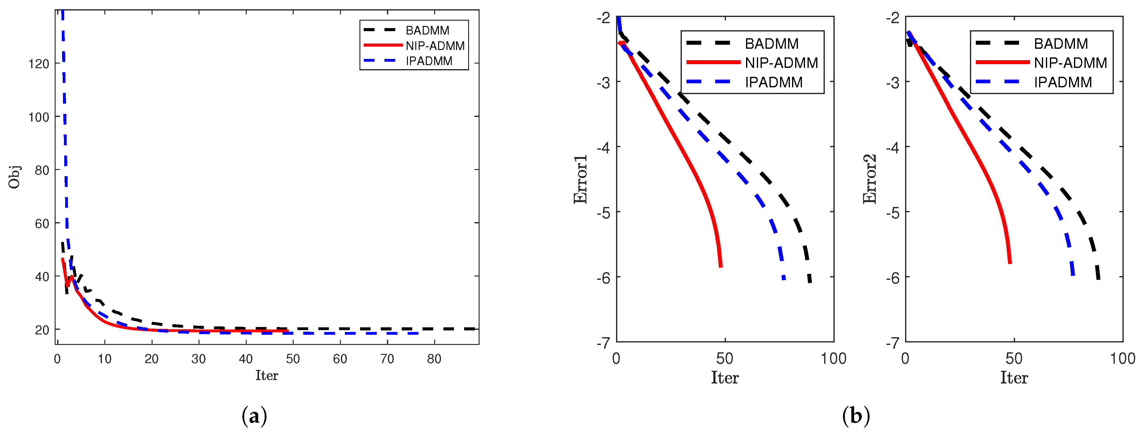
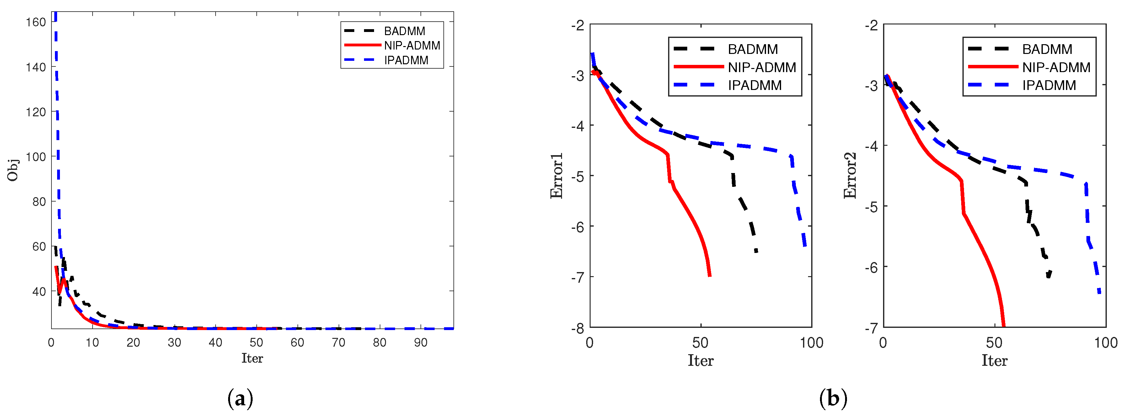
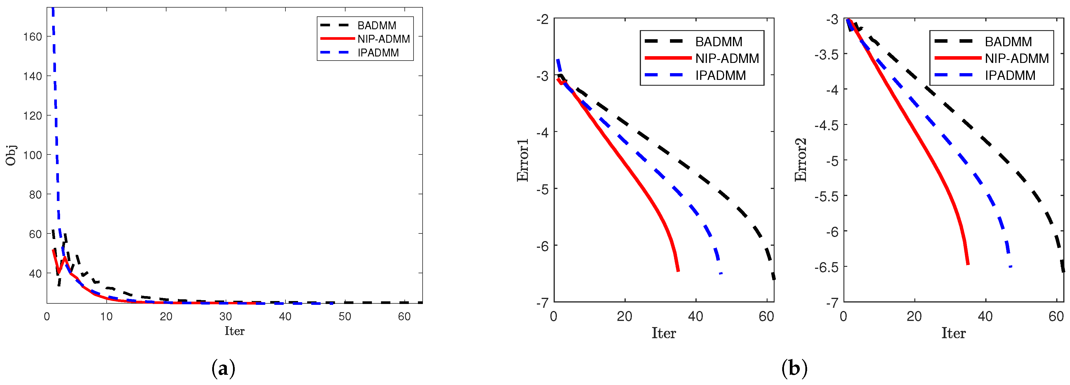
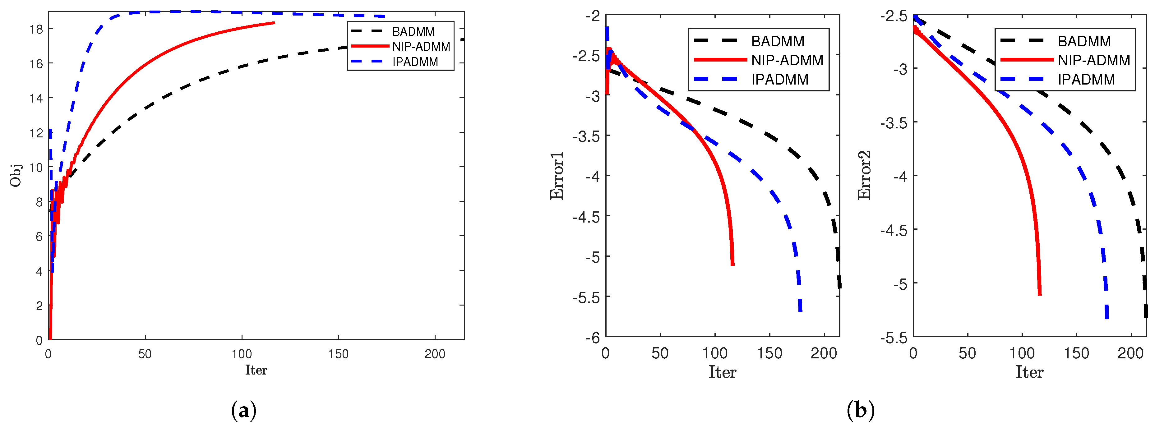
4. Numerical Simulations

In this section, we demonstrate the application of NIP-ADMM to the signal recovery model (3) and SCAD penalty problem (5). To verify the effectiveness of Algorithm 1 (i.e., NIP-ADMM), we compare it with Bregman modification of ADMM (BADMM) proposed by Wang et al. [23] and inertial proximal ADMM (IPADMM) proposed by Chen et al. [34]. All codes were implemented in MATLAB 2024b and executed on a Windows 11 system equipped with an AMD Ryzen R9-9900X CPU.

4.1. Signal Recovery

In this subsection on signal recovery, we consider the previously mentioned model (3).

$$\begin{array}{c}minc{\parallel x\parallel }_{\frac{1}{2}}^{\frac{1}{2}}+\frac{1}{2}{\parallel z\parallel }^2\\ \mathrm{s}.\mathrm{t}. Ax-z=b,\end{array}$$

(24)

where ${\parallel x\parallel }_{\frac{1}{2}}^{\frac{1}{2}}={\sum }_{i=1}^n{\left|x_i\right|}^{\frac{1}{2}}$, and $A\in {\mathbb{R}}^{m\times n},b\in {\mathbb{R}}^m$,$z\in {\mathbb{R}}^m$, $x\in {\mathbb{R}}^n$. In the context of the problem (24), Wang et al. [23] experimentally validated the effectiveness of BADMM. To further evaluate the efficiency of NIP-ADMM, numerical comparisons were conducted not only with BADMM by us, but also with IPADMM [34], to verify the rationality of the proposed inertial symmetric update scheme.

We construct the following framework to solve the problem (24). We set $S=e_{0}I-\beta A^{\top }A$, where I denotes the identity matrix.

$$\left\{\begin{array}{ll}\hfill & ({\overline{x}}^k,{\overline{z}}^k)=(x^k,z^k)+\theta (x^k-{\overline{x}}^{k-1},0)+\eta (0,z^k-{\overline{z}}^{k-1}),\hfill \\ \hfill & x^{k+1}=H\left({\displaystyle \frac{1}{e_0}}\left(-A^{\top }{\lambda }^k+\beta A^{\top }({\overline{z}}^k+b)+(e_{0}I-\beta A^{\top }A){\overline{x}}^k\right),{\displaystyle \frac{2c}{e_0}}\right),\hfill \\ \hfill & z^{k+1}=z^k-\gamma (z^k+{\lambda }^k-\beta (A{x}^{k+1}-z^k-b)),\hfill \\ \hfill & {\lambda }^{k+1}={\lambda }^k+\beta (A{x}^{k+1}-z^{k+1}-b).\hfill \end{array}\right.$$

Here, H represents the half-shrinkage operator proposed by Xu et al. [39], which is defined as

$$H(x,e)={\{h_e\left(x_1\right),h_e\left(x_2\right),\dots ,h_e\left(x_n\right)\}}^T,$$

where the function $h_e\left(x_i\right)$ for $i=1,2,\dots ,n$ is defined by

$$\left\{\begin{array}{cc}{h}_e\left(x_i\right)={\displaystyle \frac{2x_i}{3}}\left(1+cos{\displaystyle \frac{2}{3}}\left(\pi -arccos\left({\displaystyle \frac{e}{8}}{\left({\displaystyle \frac{x_i}{3}}\right)}^{-{\displaystyle \frac{3}{2}}}\right)\right)\right),\hfill & \left|x_i\right|>{\displaystyle \frac{\sqrt[3]{54}}{4}}{e}^{{\displaystyle \frac{2}{3}}},\hfill \\ 0,\hfill & \mathrm{otherwise}.\hfill \end{array}\right.$$

In this setup, the entries of matrix A are drawn from a standard normal distribution, with each column adjusted for normalization. The starting vector $x_0$ is initialized as a sparse vector, containing at least 100 non-zero components. The values ${\overline{x}}^0,{\overline{z}}^0,x^1,z^1,{\lambda }^0$ are set initially to zero. To simulate the observation vector with added noise, we generate b using $b=A{x}^0+v$, where $v\sim N(0,{10}^{-3}I)$. For the regularization parameter c, we compute

$$c=0.1\parallel A^T{b\parallel }_{\infty }.$$

Based on Assumption 1, the parameters are chosen as $\beta =3$ and $e_0=10$. The error trend is depicted as

$$\left\{\begin{array}{cc}\hfill \mathrm{Error}1=& log\parallel x^k-x^{★}\parallel ,\hfill \\ \hfill \mathrm{Error}2=& log\parallel z^k-z^{★}\parallel ,\hfill \end{array}\right.$$

where log denotes the base-10 logarithm. At the $(k+1)$-th iteration, the primal residual is expressed as $r^{k+1}=A{x}^{k+1}+z^{k+1}-b,$ while dual residual is represented as $s^{k+1}=\beta A^T(x^{k+1}-x^k).$ Termination occurs when both conditions are met:

$$\left\{\begin{array}{cc}\hfill \parallel r^{k+1}{\parallel }_2& \le \sqrt{n}\times {10}^{-4}+{10}^{-3}·max\left(\parallel A{x}^k{\parallel }_2,{\parallel z^k\parallel }_2\right),\hfill \\ \hfill \parallel s^{k+1}{\parallel }_2& \le \sqrt{n}\times {10}^{-4}+{10}^{-3}·{\parallel A^T{\lambda }^k\parallel }_2.\hfill \end{array}\right.$$

During the experiments, to satisfy Assumption 1, we set $\gamma =0.3$.

Table 1. Numerical results of NIP-ADMM with different $\theta$ and $\eta$.

$\mathit{\theta }$	$\mathit{\eta }$	Iter	CPUT(s)	$\mathit{\theta }$	$\mathit{\eta }$	Iter	CPUT(s)
0.2	0.2	75	2.2392	0.6	0.7	54	1.6014
0.3	0.2	78	2.3039	0.8	0.8	49	1.4583
0.3	0.3	69	1.9476	0.8	0.75	49	1.4309
0.5	0.5	60	1.7622	0.85	0.85	56	1.6445
0.6	0.6	56	1.6516	0.9	0.9	84	2.4614

shows that when $m=n=1000$, selecting the inertial parameter values $\theta =0.8$ and $\eta =0.75$ produces satisfactory results. Therefore, in subsequent experiments, we also adopt $\theta =0.8$ and $\eta =0.75$. The metrics include the number of iterations (Iter), CPU running time (CPUT) and the objective function value (Obj). To better present the experimental results, we retain two decimal places for Obj and four decimal places for CPUT.

The numerical results consistently demonstrate the superior performance of NIP-ADMM compared to BADMM and IPADMM (see

Table 2. Comparison of iteration effect between NIP-ADMM, IPADMM and BADMM.

m	n	NIP-ADMM			IPADMM			BADMM
		Iter	CPUT(s)	Obj	Iter	CPUT(s)	Obj	Iter	CPUT(s)	Obj
1000	1000	49	1.2698	19.36	78	2.1407	18.46	90	2.3407	20.14
1500	2000	44	4.9152	23.17	72	8.4978	22.12	76	8.5387	23.69
3000	3000	40	15.0464	21.02	57	22.3823	20.56	73	27.4115	21.18
3000	4000	55	34.0601	23.21	98	62.8206	23.11	76	48.3825	23.22
4000	5000	36	40.6110	24.02	53	61.7431	23.09	65	74.4521	24.03
4500	5500	40	61.7638	24.05	45	71.7627	23.79	67	102.6028	24.06
6000	6000	40	88.7702	24.99	48	108.3045	24.56	63	135.8133	25.00

). Due to the introduction of inertial and proximal terms, the proposed NIP-ADMM demonstrates accelerated convergence with respect to both objective value reduction and error diminution. For $m=n=1000$, NIP-ADMM shows faster convergence in terms of both objective value and error reduction (see Figure 1). For $m=3000$ and $n=4000$, in comparison to BADMM and IPADMM, NIP-ADMM achieves a more significant reduction in the number of iterations and computational time (see Figure 2). For larger-scale models with $m=n=6000$, NIP-ADMM consistently outperforms both BADMM and IPADMM, further indicating its superior suitability for solving large-scale problems (see Figure 3). It is worth noting that the above results highlight the high efficiency of NIP-ADMM, which can be attributed to the proposed inertial update strategy.

4.2. SCAD Penalty Problem

We note that the SCAD penalty problem in statistics can be formulated as the following model [20,31]:

$$\begin{array}{cc}\hfill min& \sum _{i=1}^n{h}_k\left(\right|x_i\left|\right)+{\displaystyle \frac{1}{2}}{\parallel p\parallel }^2\hfill \\ \hfill \mathrm{s}.\mathrm{t}.& Ax-p=b,\hfill \end{array}$$

(25)

with $A\in {\mathbb{R}}^{m\times n},b\in {\mathbb{R}}^m$,$p\in {\mathbb{R}}^m$, $x\in {\mathbb{R}}^n$ and the penalty function $h_{\kappa }$ in the objective defined as

$$h_{\kappa }\left(\theta \right)=\left\{\begin{array}{cc}\kappa \theta ,\hfill & \theta \le \kappa ,\hfill \\ {\displaystyle \frac{-{\theta }^2+2c\kappa \theta -{\kappa }^2}{2(c+1)}},\hfill & \kappa <\theta \le c\kappa ,\hfill \\ {\displaystyle \frac{(c+1){\kappa }^2}{2}},\hfill & \theta >c\kappa ,\hfill \end{array}\right.$$

(26)

where $c>2$ and $\kappa >0$, being the knots of the quadratic spline function. In the reference signal recovery subsection, we similarly set $\psi \left(x\right)={\displaystyle \frac{1}{2}}{\parallel x\parallel }_S^2$ and $\varphi \left(y\right)=0$, where $S=\mu I-\beta A^{\top }A$. For the problem (25), the x-subproblem corresponding to $2^{\circ }$ of Algorithm 1 can be expressed as

$$\begin{array}{cc}\hfill x^{k+1}& =argmin\left\{{\sum }_{i=1}^n{h}_k\left(\right|x_i\left|\right)-\langle {\lambda }^k,Ax\rangle +{\displaystyle \frac{\beta }{2}}\parallel Ax-{\overline{p}}^k{-b\parallel }^2+{\displaystyle \frac{1}{2}}{\parallel x-{\overline{x}}^k\parallel }_{\mu I-\beta A^{T}A}^2\right\}\\ \hfill & =argmin\left\{{\sum }_{i=1}^n{h}_k\left(\right|x_i\left|\right)+{\displaystyle \frac{\mu }{2}}{∥x-{\displaystyle \frac{\beta A^T({\overline{p}}^k+b+\frac{p^k}{\beta }-A{\overline{x}}^k)}{\mu }}∥}^2\right\}.\end{array}$$

On the one hand, the x-subproblem can be equivalently formulated as:

$$\underset{x\in {\mathbb{R}}^n}{min}\left\{\sum _{i=1}^n{h}_k\left(\right|x_i\left|\right)+{\displaystyle \frac{1}{2\nu }}{\parallel x-q\parallel }^2\right\}.$$

On the other hand, under the condition that $1+\nu \le c$, we can update x using the following rule [31]:

$$x_i:=\left\{\begin{array}{cc}\mathrm{sign}\left(q_i\right)\left(\right|q_i{|-\kappa \nu )}_{+},\hfill & |q_i|\le (1+\nu )\kappa ,\hfill \\ {\displaystyle \frac{(c-1)q_i-\mathrm{sign}\left(q_i\right)\kappa \nu }{c-1-\nu }},\hfill & (1+\nu )\kappa <|q_i|\le c\kappa ,\hfill \\ q_i,\hfill & |q_i|>c\kappa ,\hfill \end{array}\right.$$

where ${(·)}_{+}$ represents the positive part operator, which is defined as ${\left(x\right)}_{+}=max(0,x)$; applying NIP-ADMM to solve the problem (25), one yields that

$$\left\{\begin{array}{c}{\overline{x}}^k=x^k+\theta (x^k-{\overline{x}}^{k-1}),{\overline{p}}^k=p^k+\eta (p^k-{\overline{y}}^{k-1}),\hfill \\ x^{k+1}=argmin\left\{\sum _{i=1}^n{h}_k\left(\right|x_i\left|\right)+{\displaystyle \frac{\mu }{2}}{\parallel x-{\displaystyle \frac{-A^{\top }{\lambda }^k+\beta A^{\top }({\overline{p}}^k+b)+{\mu }_0{\overline{x}}^k-A^{\top }A{\overline{x}}^k}{\mu }}\parallel }^2\right\},\hfill \\ p^{k+1}=p^k-\gamma (p^k-{\lambda }^k-\beta (A{x}^{k+1}-p^k-b)),\hfill \\ {\lambda }^{k+1}={\lambda }^k-\beta (A{x}^{k+1}-p^{k+1}-b).\hfill \end{array}\right.$$

Similarly, the update scheme of BADMM can be represented by the following procedure:

$$\left\{\begin{array}{c}{x}^{k+1}=argmin\left\{\sum _{i=1}^n{h}_k\left(\right|x_i\left|\right)+{\displaystyle \frac{\mu }{2}}{\parallel x-{\displaystyle \frac{\beta A^T(p^k+b+\frac{{\lambda }^k}{\beta }-A{x}^k)+\mu x^k}{\mu }}\parallel }^2\right\},\hfill \\ p^{k+1}={\displaystyle \frac{1}{1+\beta }}\left(\beta (A{x}^{k+1}-b)-{\lambda }^k\right),\hfill \\ {\lambda }^{k+1}={\lambda }^k-\beta (A{x}^{k+1}-p^{k+1}-b).\hfill \end{array}\right.$$

Utilize IPADMM to address model (25) and derive the following iterative scheme:

$$\left\{\begin{array}{c}({\overline{x}}^k,{\overline{p}}^k,{\overline{\lambda }}^k)=(x^k,p^k,{\lambda }^k)+\theta (x^k-x^{k-1},p^k-p^{k-1},{\lambda }^k-{\lambda }^{k-1}),,\hfill \\ x^{k+1}=argmin\left\{\sum _{i=1}^n{h}_k\left(\right|x_i\left|\right)+{\displaystyle \frac{\mu }{2}}{\parallel x-{\displaystyle \frac{-A^{\top }{\overline{\lambda }}^k+\beta A^{\top }({\overline{p}}^k+b)+{\mu }_0{\overline{x}}^k-A^{\top }A{\overline{x}}^k}{\mu }}\parallel }^2\right\},\hfill \\ {\lambda }^{k+1}={\overline{\lambda }}^k-\beta (A{x}^{k+1}-{\overline{p}}^k-b),\hfill \\ p^{k+1}={\displaystyle \frac{1}{1+\beta }}\left(\beta (A{x}^{k+1}-b)-{\lambda }^k\right).\hfill \end{array}\right.$$

In this experiment, we generate a random $m\times n$ matrix A, and perform row and column normalization. Here, we choose to generate a vector z of dimension n with a sparsity ratio of ${\displaystyle \frac{100}{m}}$. The vector b is represented as the sum of $Az$ and a Gaussian noise vector with zero mean and variance $0.001$. The initial variables $x_1$, $x_0$, $p_1$ and $p_0$ are set as zero vectors, serving as the starting point for optimization. To improve numerical efficiency, in this experiment, we set $c=5$ and $\kappa =0.1$. Under the condition that Assumption 1 is satisfied, we configure $\gamma =0.1$, $\beta =12$, and $\mu =100$ for NIP-ADMM and other algorithms. The error trend is depicted as

$$\left\{\begin{array}{cc}\hfill \mathrm{Error}1=& log\parallel x^k-x^{★}\parallel ,\hfill \\ \hfill \mathrm{Error}2=& log\parallel p^k-p^{★}\parallel ,\hfill \end{array}\right.$$

and the stopping criterion for the updates is set as

$$max\left\{\parallel x^{k+1}-x^k\parallel ,\parallel p^{k+1}-p^k\parallel \right\}\le {10}^{-2}.$$

In

Table 3. Numerical results of NIP-ADMM with different $\theta$ and $\eta$.

$\mathit{\theta }$	$\mathit{\eta }$	Iter	CPUT(s)	$\mathit{\theta }$	$\mathit{\eta }$	Iter	CPUT(s)
0.2	0.2	196	2.0092	0.6	0.7	149	1.5017
0.3	0.2	187	1.9122	0.8	0.7	134	1.3693
0.3	0.3	181	1.8690	0.8	0.9	133	1.3503
0.4	0.5	170	1.7650	0.9	0.8	127	1.3467
0.5	0.5	159	1.6438	0.9	0.9	126	1.3100

, we set $m=n=1000$. The results in the table support our choice of the inertial parameters $\eta =0.9$ and $\theta =0.9$. Under these conditions, NIP-ADMM requires the fewest iterations and the least running time. Therefore, we selected the inertial parameters $\eta =0.9$ and $\theta =0.9$ for the experiments.

To further evaluate the performance of NIP-ADMM, IPADMM, and BADMM in solving the SCAD penalized problem, we conducted numerical experiments under three different dimensional settings and compared the convergence behavior of the three algorithms. Figure 4, Figure 5 and Figure 6 illustrate the evolution of the objective function values (left) and iteration errors (right) with respect to the number of iterations for NIP-ADMM, IPADMM, and BADMM. As observed from the figures, although all three algorithms eventually converge, NIP-ADMM demonstrates superior performance in terms of convergence speed and error control. In addition,

Table 4. Comparison of iteration effect between NIP-ADMM, IPADMM and BADMM.

m	n	NIP-ADMM			IPADMM			BADMM
		Iter	CPUT(s)	Obj	Iter	CPUT(s)	Obj	Iter	CPUT(s)	Obj
1000	1000	121	1.3366	10.91	213	2.3065	10.55	182	1.9632	10.55
1000	1300	115	1.9246	12.96	211	3.5724	12.48	174	2.9611	13.13
1500	1000	130	1.9270	8.92	228	3.2943	8.59	172	2.4709	7.49
1500	1300	140	3.0474	13.38	259	5.7832	12.90	215	4.7147	11.88
1500	1500	125	3.6104	13.43	230	6.6865	12.81	196	5.4584	12.71
1800	1500	146	4.6432	13.47	257	8.0396	12.94	209	6.1925	11.83
1800	2000	115	5.8341	15.00	210	10.7513	14.29	182	9.1033	14.69
2500	2000	142	8.9043	14.95	250	15.6397	14.29	201	12.2370	13.07
2900	2700	134	15.3647	17.70	245	28.4289	16.71	203	22.9945	16.50
3000	3000	125	17.1686	17.20	217	34.1575	16.34	188	25.0864	17.22
3500	3000	128	20.2808	16.87	234	37.1725	15.84	194	30.6876	15.94
3500	3500	123	24.5455	19.80	223	44.4163	18.69	200	39.2771	19.43

presents the numerical performance of the three algorithms under different dimensional settings. Although there are slight differences in the objective function values among the three methods, NIP-ADMM exhibits a clear advantage in terms of iteration count (Iter) and computational time (CPUT). These results clearly demonstrate the acceleration effect brought by the incorporation of inertial and proximal terms in NIP-ADMM.

5. Conclusions

In this paper, we studied a class of nonconvex optimization problems subject to linear constraints. By integrating a class of symmetrically structured inertial terms with a proximal ADMM framework, we proposed a novel symmetrical inertial alternating direction method of multipliers with a proximal term. Under some mild assumptions, we analyzed the subsequential convergence of the proposed NIP-ADMM. Furthermore, assuming that the associated auxiliary function satisfied Kurdyka–Łojasiewicz property, we established the global convergence of the algorithm, which provided theoretical support for the stability of the algorithm. Meanwhile, numerical simulations also validated the theoretical contributions. In both the signal recovery problem and SCAD-penalized problem, NIP-ADMM demonstrated faster convergence compared to IPADMM and BADMM. These results not only confirmed the theoretical advantages of the symmetric inertial term in accelerating convergence and the proximal term in simplifying subproblem computations, but also indicated that NIP-ADMM outperformed both non-inertial and traditional inertial methods in practical applications.

Furthermore, we believe that future work could explore whether the convergence of NIP-ADMM can be guaranteed when the objective function is non-separable. Additionally, it would be worthwhile to investigate whether introducing inertial terms into the y-subproblem and the multiplier $\lambda$ could further accelerate the convergence speed of NIP-ADMM.

References

1. Kim, S.J.; Koh, K.; Lustig, M.; Boyd, S.; Gorinevsky, D. An interior-point method for large-scale 1-regularized least Squares. IEEE J. Sel. Top. Signal Process. 2007, 1, 606–617. [Google Scholar] [CrossRef]
2. Chartrand, R.; Staneva, V. Restricted isometry properties and nonconvex compressive sensing. Inverse Probl. 2008, 24, 035020. [Google Scholar] [CrossRef]
3. Zeng, J.S.; Lin, S.B.; Wang, Y.; Xu, Z.B. L1/2 regularization: Convergence of iterative half thresholding algorithm. IEEE Trans. Signal Process. 2014, 62, 2317–2329. [Google Scholar] [CrossRef]
4. Doostmohammadian, M.; Gabidullina, Z.R.; Rabiee, H.R. Nonlinear perturbation-based non-convex optimization over time-varying networks. IEEE Trans. Netw. Sci. Eng. 2024, 11, 6461–6469. [Google Scholar] [CrossRef]
5. Chen, P.Y.; Selesnick, I.W. Group-sparse signal denoising: Non-convex regularization, convex optimization. IEEE Trans. Signal Process. 2014, 62, 3464–3478. [Google Scholar] [CrossRef]
6. Bai, Z.L. Sparse Bayesian learning for sparse signal recovery using 1/2-norm. Appl. Acoust. 2023, 207, 109340. [Google Scholar] [CrossRef]
7. Wang, C.; Yan, M.; Rahimi, Y.; Lou, Y.F. Accelerated schemes for the L1/L2 minimization. IEEE Trans. Signal Process. 2020, 68, 2660–2669. [Google Scholar] [CrossRef]
8. Zhang, S.R.; Wang, Q.H.; Zhang, B.X.; Liang, Z.; Zhang, L.; Li, L.L.; Huang, G.; Zhang, Z.G.; Feng, B.; Yu, T.Y. Cauchy non-convex sparse feature selection method for the high-dimensional small-sample problem in motor imagery EEG decoding. Front. Neurosci. 2023, 17, 1292724. [Google Scholar] [CrossRef]
9. Tiddeman, B.; Ghahremani, M. Principal component wavelet networks for solving linear inverse problems. Symmetry 2021, 13, 1083. [Google Scholar] [CrossRef]
10. Xia, Z.C.; Liu, Y.; Hu, C.; Jiang, H.J. Distributed nonconvex optimization subject to globally coupled constraints via collaborative neurodynamic optimization. Neural Netw. 2025, 184, 107027. [Google Scholar] [CrossRef]
11. Yu, G.; Fu, H.; Liu, Y.F. High-dimensional cost-constrained regression via nonconvex optimization. Technometrics 2021, 64, 52–64. [Google Scholar] [CrossRef] [PubMed]
12. Merzbacher, C.; Mac Aodha, O.; Oyarzun, D.A. Bayesian optimization for design of multiscale biological circuits. ACS Synth. Biol. 2023, 12, 2073–2082. [Google Scholar] [CrossRef] [PubMed]
13. Bai, J.C.; Zhang, H.C.; Li, J.C. A parameterized proximal point algorithm for separable convex optimization. Optim. Lett. 2018, 12, 1589–1608. [Google Scholar] [CrossRef]
14. Wen, F.; Liu, P.L.; Liu, Y.P.; Qiu, R.C.; Yu, W.X. Robust sparse recovery in impulsive noise via p-1 optimization. IEEE Trans. Signal Process. 2017, 65, 105–118. [Google Scholar] [CrossRef]
15. Zhang, H.M.; Gao, J.B.; Qian, J.J.; Yang, J.; Xu, C.Y.; Zhang, B. Linear regression problem relaxations solved by nonconvex ADMM with convergence analysis. IEEE Trans. Circuits Syst. Video Technol. 2023, 34, 828–838. [Google Scholar] [CrossRef]
16. Ames, B.P.W.; Hong, M.Y. Alternating direction method of multipliers for penalized zero-variance discriminant analysis. Comput. Optim. Appl. 2016, 64, 725–754. [Google Scholar] [CrossRef]
17. Zietlow, C.; Lindner, J.K.N. ADMM-TGV image restoration for scientific applications with unbiased parameter choice. Numer. Algorithms 2024, 97, 1481–1512. [Google Scholar] [CrossRef]
18. Bian, F.M.; Liang, J.W.; Zhang, X.Q. A stochastic alternating direction method of multipliers for non-smooth and non-convex optimization. Inverse Probl. 2021, 37, 075009. [Google Scholar] [CrossRef]
19. Beck, A.; Teboulle, M. A fast iterative shrinkage-thresholding algorithm for linear inverse problems. SIAM J. Imaging Sci. 2009, 2, 183–202. [Google Scholar] [CrossRef]
20. Fan, J.Q.; Li, R.Z. Variable selection via nonconcave penalized likelihood and its oracle properties. J. Am. Statist. Assoc. 2001, 96, 1348–1360. [Google Scholar] [CrossRef]
21. Parikh, N.; Boyd, S. Proximal Algorithms; Now Publishers: Braintree, MA, USA, 2014. [Google Scholar]
22. Hong, M.Y.; Luo, Z.Q.; Razaviyayn, M. Convergence analysis of alternating direction method of multipliers for a family of nonconvex problems. SIAM J. Optim. 2016, 26, 337–364. [Google Scholar] [CrossRef]
23. Wang, F.H.; Xu, Z.B.; Xu, H.K. Convergence of Bregman alternating direction method with multipliers for nonconvex composite problems. arXiv 2014, arXiv:1410.8625. [Google Scholar]
24. Ding, W.; Shang, Y.; Jin, Z.; Fan, Y. Semi-proximal ADMM for primal and dual robust Low-Rank matrix restoration from corrupted observations. Symmetry 2024, 16, 303. [Google Scholar] [CrossRef]
25. Guo, K.; Han, D.R.; Wu, T.T. Convergence of alternating direction method for minimizing sum of two nonconvex functions with linear constraints. Int. J. Comput. Math. 2016, 94, 1653–1669. [Google Scholar] [CrossRef]
26. Wang, Y.; Yin, W.T.; Zeng, J.S. Global convergence of ADMM in nonconvex nonsmooth optimization. J. Sci. Comput. 2019, 78, 29–63. [Google Scholar] [CrossRef]
27. Wang, F.H.; Cao, W.F.; Xu, Z.B. Convergence of multi-block Bregman ADMM for nonconvex composite problems. Sci. China Inf. Sci. 2018, 61, 122101. [Google Scholar] [CrossRef]
28. Barber, R.F.; Sidky, E.Y. Convergence for nonconvex ADMM, with applications to CT imaging. J. Mach. Learn. Res. 2024, 25, 1–46. [Google Scholar]
29. Wang, X.F.; Yan, J.C.; Jin, B.; Li, W.H. Distributed and parallel ADMM for structured nonconvex optimization problem. IEEE Trans. Cybern. 2021, 51, 4540–4552. [Google Scholar] [CrossRef]
30. Alvarez, F.; Attouch, H. An inertial proximal method for maximal monotone operators via discretization of a nonlinear oscillator with damping. Set-Valued Anal. 2001, 9, 3–11. [Google Scholar] [CrossRef]
31. Wu, Z.M.; Li, M. General inertial proximal gradient method for a class of nonconvex nonsmooth optimization problems. Comput. Optim. Appl. 2019, 73, 129–158. [Google Scholar] [CrossRef]
32. Chao, M.T.; Zhang, Y.; Jian, J.B. An inertial proximal alternating direction method of multipliers for nonconvex optimization. Int. J. Comput. Math. 2020, 98, 1199–1217. [Google Scholar] [CrossRef]
33. Wang, X.Q.; Shao, H.; Liu, P.J.; Wu, T. An inertial proximal partially symmetric ADMM-based algorithm for linearly constrained multi-block nonconvex optimization problems with applications. J. Comput. Appl. Math. 2023, 420, 114821. [Google Scholar] [CrossRef]
34. Chen, C.H.; Chan, R.H.; Ma, S.Q.; Yang, J.F. Inertial proximal ADMM for linearly constrained separable convex optimization. SIAM J. Imaging Sci. 2015, 8, 2239–2267. [Google Scholar] [CrossRef]
35. Attouch, H.; Bolte, J.; Redont, P.; Soubeyran, A. Proximal alternating minimization and projection methods for nonconvex problems: An approach based on the Kurdyka-Łojasiewicz inequality. Math. Oper. Res. 2010, 35, 438–457. [Google Scholar] [CrossRef]
36. Rockafellar, R.T.; Wets, R.J.B. Variational Analysis; Springer: Berlin, Germany, 1998. [Google Scholar]
37. Bolte, J.; Sabach, S.; Teboulle, M. Proximal alternating linearized minimization for nonconvex and nonsmooth problems. Math. Program. 2014, 146, 459–494. [Google Scholar] [CrossRef]
38. Nesterov, Y. Introductory Lectures on Convex Optimization: A Basic Course; Springer: New York, NY, USA, 2004. [Google Scholar]
39. Xu, Z.B.; Chang, X.Y.; Xu, F.M.; Zhang, H. L1/2 regularization: A thresholding representation theory and a fast solver. IEEE Trans. Neural Netw. Learn. Syst. 2012, 23, 1013–1027. [Google Scholar] [CrossRef]
Figure 1. Comparison of convergence when m = n = 1000 : (a) The objective value. (b) The error trends of Error1 and Error2.
Symmetry 17 00887 g001
Figure 2. Comparison of convergence when m = 3000 and n = 4000 : (a) The objective value. (b) The error trends of Error1 and Error2.
Symmetry 17 00887 g002
Figure 3. Comparison of convergence when m = n = 6000: (a) The objective value. (b) The error trends of Error1 and Error2.
Symmetry 17 00887 g003
Figure 4. Comparison of convergence when m = n = 1500 : (a) The objective value. (b) The error trends of Error1 and Error2.
Symmetry 17 00887 g004
Figure 5. Comparison of convergence when m = 2000 and n = 2500 : (a) The objective value. (b) The error trends of Error1 and Error2.
Symmetry 17 00887 g005
Figure 6. Comparison of convergence when m = n = 3500 : (a) The objective value. (b) The error trends of Error1 and Error2.
Symmetry 17 00887 g006