Three-Dimensional and Oblique Wave-Current Interaction with a Floating Elastic Plate Based on an Analytical Approach

Abstract

An analytical hydroelastic model formulation in three-dimensional and oblique wave cases is developed to analyze the dynamic response of a horizontal, floating elastic plate subject to wave-current interaction under linearized small-amplitude wave theory. The floating elastic plate is moored to the bottom bed and free to the channel walls. Green’s function’s technique is utilised to determine the dispersion relation in 3D, and the series form of Green’s function in different water depths is derived in the oblique wave case. Further, the comparative analysis of phase and group velocities for different wave angles, between the present the existing models, is discussed. The derived dispersion relation is used in the solution by applying the geometrical symmetry velocity decomposition method. The present theoretical results of wave quantities are validated with the recently published and existing numerical hydroelastic model. A comparative analysis revealed a 1.7% difference between the present model and the existing hydroelastic models, and a 7.7% difference when compared to the model’s limiting cases. Several numerical results of the wave quantities, wave force, and vertical displacements are conducted to investigate the influence of current velocity on the hydroelastic response in three dimensions. It has been noted that the value of reflection coefficient diminishes for larger values of current velocity and the vertical displacement correspondingly becomes greater. This analysis will inform the design of elastic plate-based wave energy converters and breakwaters by clarifying how current loads affect the hydroelastic of a floating elastic plate with an oblique angle and three dimensions.

1. Introduction

Nowadays, environmental parameters are a key consideration in the engineering design of marine structures. Considering the structural integrity of elastic materials in marine environments, particularly under the stress of strong waves, currents, and varying depths, is crucial. Economical construction depends on understanding these elastic properties, when shielded from seismic activity, does not harm the marine environment or impede ocean currents, and can be removed or expanded effortlessly and, therefore, is environmentally sustainable. These types of structures have a considerable application to offshore ports, pontoons, offshore airports, and other facilities that enhance maritime trade and breakwaters [1,2,3].

On the other hand, the use of flexible marine structures has attracted increasing attention recently [4,5]. A few studies have been carried out to analyze the response for energy harvesting when it is attached to marine equipment. For instance, the hydroelastic behavior of the floating flexible plate attached with a linear damper for Wave Energy Converter (WEC) under monochromatic waves was analyzed analytically [6]. The application of a floating flexible horizontal membrane connected with linear springs to WEC based on analytical and experimental studies was studied [7]. The submerged plate wave energy conversion based on mathematical and numerical methods was presented in [8].

Wu et al. [9] studied the wave-induced response of an elastic floating plate by employing the modal expansion method for structural motion. By using the mode expansion method, Chen et al. [10] studied the first-order vertical displacement subjected to regular multi-directional waves based on hydroelastic analysis. The hydroelastic behavior of a floating elastic platform of finite length was analyzed based on the thin plate theory under analytical and numerical methods in a finite water depth [11]. Papathanasiou and Belibassakis [12] studied the hydroelastic response of a floating slender plate in shallow water over variable topography under finite element solution. Iijima et al. [13] addressed the deflection waves on a floating thin elastic plate by conducting a series of tests, and the results were compared with numerical model simulations.

The bending moment and the shear force of a rectangular floating plate were studied in a shallow water regime and thin plate theory in [14]. The hydroelastic behavior of a 2D floating elastic plate (FEP) under regular waves was studied by analyzing the deflection and motion response in finite water depth [15]. The behavior of a floating semi-infinite plate in surface waves was based on the Wiener–Hopf technique in [16]. By applying the Wiener–Hopf technique, in the finite water depth, the plate displacement and bending moment were analyzed and the results were compared with experimental datasets [17]. Using the Green–Naghdi (GN) theory, the hydroelastic response of a very long plate with finite width was analyzed, and the findings were compared with experimental data sets available in the literature [18]. The response of an infinitely floating viscoelastic plate due to wave resistance by a point load was studied analytically under the Fourier integral transform method in [19]. The deflections and strain of a floating elastic ice plate with a vertical rigid plate were studied analytically in 2D by modeling a hydroelastic problem [20]. The hydroelastic solitary waves over a thin elastic plate modeled as the Euler–Bernoulli beam were studied analytically using the Poincaré–Lighthill–Kuo method [21]. The hydrodynamic force and wave quantities were studied analytically for a floating rectangular plate subjected to surface wave conditions under the Kirchhoff–Love plate theory [22]. The explicit analytical solution for a plane problem of one-dimensional nature of surface wave interaction with an elastic plate was provided in [23,24]. Based on the linear theory of hydroelasticity, a three-dimensional model associated with ice-covered rectangular cross-section is solved, where the ice deflection is caused by an underwater body moving along a frozen channel [25].

Under current conditions, using the higher-order BEM, Huang et al. [26] explored the hydrodynamic behavior of 3D bodies with arbitrary shapes when exposed to waves and weak currents within a channel. An analytical approach [27] was used to examine the impact of a uniform underlying current on the nonlinear hydroelastic waves generated by an infinitely long floating plate. Liang et al. [28] studied the second harmonic displacement of a 2D large elastic plate based on the fully nonlinear numerical wave tank. The nonlinear hydroelastic analysis of a FEP in terms of plate deflection under current loads was studied analytically in deep water by using the homotopy analysis method [29].

The impact of various design parameters and modes on the displacement and wave quantities on the FEP with submerged flexible structure in 3D is analyzed [30]. Further, the wave-current interaction with the floating flexible membrane in three dimensions based on an analytical approach was developed [7]. While advancements in the FEP model have occurred, the impact of current velocity (CV) on a 3D analytical hydroelastic model associated with the FEP connected with a cable remains absent. A key benefit of this model is its ability to explain the relationship between currents and FEP’s hydroelastic behavior. Hence, the purpose of this research is to present a 3D analytical hydroelastic model that accounts for currents, offering analytical results and valuable perspectives to the existing body of knowledge.

It may be noted that the geometrical symmetry velocity decomposition method is advantageous because: (i) orthogonal eigenfunctions in the expansion formula simplify boundary value problems to diagonally dominant linear systems, increasing computational efficiency; (ii) symmetric relations enable extending solutions to the entire fluid domain; and (iii) the resulting analytical solutions often reveal key physical characteristics and provide benchmark data for validating computational models.

Section 2 demonstrates the hydroelastic formulation of the mentioned model based on the linearized water wave theory in 3D under current conditions, following the goals of the study. Section 3 presents the oblique wave-current formulation and derivation of Green’s function in terms of series expansion, applying the Cauchy residue theorem in different water depths. In addition, a comparative analysis between the phase and group velocities for different oblique angles is discussed via a numerical example. Section 4 employs methods that incorporate Green’s function to derive the dispersion relation (DR) under varying water depths and current conditions. Further, a comparative study between the present and existing 3D models of the phase and group velocities is conducted. The obtained DR is subsequently employed in the 3D theoretical solution through the implementation of the geometrical symmetry velocity decomposition method in Section 5. Section 6 compares present analytical results for the wave quantities with existing published results, and the interaction of wave and current conditions on the hydroelastic behavior of the FEP is examined through numerical simulations, incorporating structural and environmental factors. Section 7 offers a summary of the study’s results and highlights potential areas for future research.

2. Hydroelastic Model Position

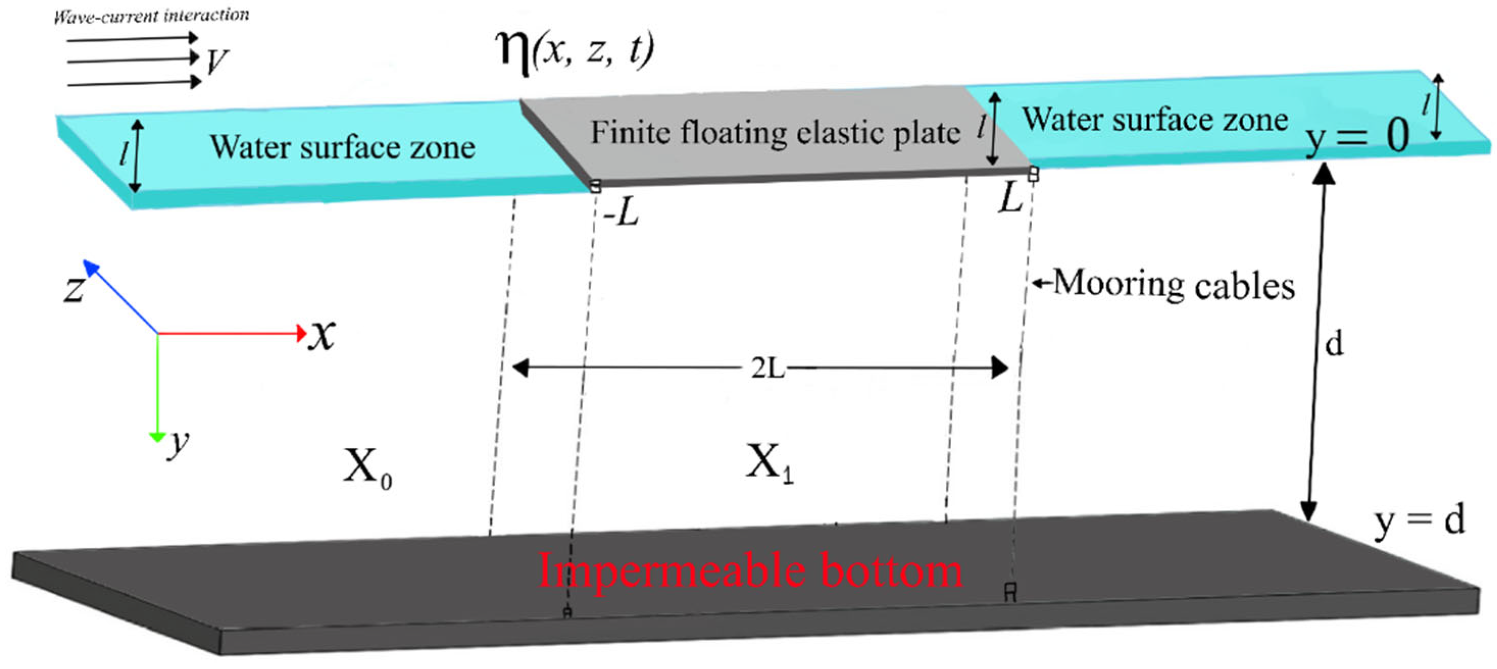
The boundary value problem of the hydroelastic model is formulated in a dimensional Cartesian coordinate system, with $x-z$ the horizontal plane and the $y-$ axis being the vertical downward positive direction in water of finite depth under linear water wave theory. The fluid zone is considered as a semi-infinitely extended channel of finite width, and the channel’s two sidewalls are assumed to be rigid.

The FEP of length $2L$ and width $l$ occupies the zone $x\in \left(-L,L\right), z\in \left[0,l\right]$ on the mean free surface $y=0$ over the impermeable bottom bed. The current velocity is in the same direction of wave propagation in the positive direction of the x- and z-axis referred to as the following current; $v_1$ and $v_2$ in x- and z-directions. As the wave-current flow in a channel is restricted by vertical walls at $z=0, l$ that results in the reflection of current flow by the side walls and could be confined to $v_1=v, v_2=0$ (as in [7]). The FEP is connected with linear elastic cables with stiffness $k_j$ for j = 1,2 at the edges of the horizontal FEP (see Figure 1).

Consequently, the fluid zone is fully characterized by:

$$\mathrm{Zone}=\left\{\begin{array}{l}x\in (-\infty ,-L)\cup (L,\infty ), y\in (0,d), \mathrm{z}\in \left[0,l\right] \mathrm{represent} {{\rm X}}_0,\\ x\in (-L,L), y\in (0,d), \mathrm{z}\in \left[0,l\right] \mathrm{signify} {{\rm X}}_1.\end{array}\right.$$

It is assumed that the fluid has no viscosity, is incompressible, and the motion is free of rotation. Thus, the total velocity potential $\mathsf{\gamma }(\overline{x};t)$ including the current condition is expressed as (see [7]):

$$\mathsf{\gamma }(\overline{x};t)=vx+\Phi (\overline{x};t)$$

(1)

where $\Phi (\overline{x};t)=\mathrm{Re}\{\varphi (\overline{x})e^{-i\omega t}\}$, and Re is the real part of the complex velocity potential with $\overline{x}=(x,y,z)$. Further, the displacement of the FEP is presumed to be of the form $\eta (x,z;t)=\mathrm{Re}\{\eta (x,z)e^{-i\omega t}\}$ and $\eta (x,z)$ is the displacement without time-harmonic assumption. Therefore, the velocity potential $\Phi \left(x;t\right)$ that satisfies the 3D Laplace equation,

$$\left({\partial }_{xx}+{\partial }_{xx}+{\partial }_{xx}\right)\Phi =0, \mathrm{in} \mathrm{the} \mathrm{fluid} \mathrm{zone}.$$

(2)

By merging the dynamic and kinematic linearized conditions (see [7]), we can derive the linear representation of the free surface boundary condition under CV, as follows:

$${\left({\partial }_t+v{\partial }_x\right)}^2{\Phi }_0+g{\Phi }_{0y}=0$$

(3)

Since the seabed is inflexible, the boundary conditions in water for Finite Depth (FD) and Infinite Depth (ID) are as follows:

$${\Phi }_y=0 \mathrm{on} y=d$$

(4a)

$$\Phi , \left|\nabla \Phi \right|\to 0 \mathrm{as} \mathrm{y}\to \infty$$

(4b)

Considering both the dynamic forces acting on the Flexible Elastic Plate (FEP) and the hydrodynamic pressure within the region defined by $x\in \left(-L, L\right), z\in \left[0,l\right]$, the linear plate-covering condition, accounting for the influence of current, can be expressed as follows:

$$\{EI{({\partial }_x^2+{\partial }_z^2)}^2+({ℂ}_x{\partial }_x^2+{ℂ}_z{\partial }_z^2)-{\rho }_{m}d{\partial }_t^2\}\eta =\rho \left({\partial }_t+v{\partial }_x\right){\Phi }_1-\rho g\eta$$

(5)

The notation uses subscripts ‘x’, ‘z’, and ‘t’ to denote partial derivatives with respect to x, z, and t, respectively. Additionally, ${ℂ}_x$ and ${ℂ}_z$ signify the compressive force exerted on the FEP in the x and z directions, respectively.

Assuming a consistent compressive force acts on the FEP along x- and z- directions, that is ${ℂ}_x={ℂ}_z=ℂ$ in Equation (5) and eliminating $\eta$ from the kinematic condition, the 5th order BC on the plate-covered zone can be derived as follows:

$${\partial }_y\left({\rm K}{\partial }_{yyyy}+\Theta {\partial }_{yy}-{\gamma }_m{\partial }_{tt}+1\right){\Phi }_1={\displaystyle \frac{1}{g}}{({\partial }_t+v{\partial }_x)}^2{\Phi }_1, x\in \left(-L,L\right), z\in \left[0,l\right],$$

(6)

where ${\rm K}=EI/\rho g$, $\Theta ={\displaystyle \frac{\mathbb{C}}{\rho g}}$ and ${\gamma }_m={\rho }_{m}d/\rho g$ with $\Theta$, ρ_m, and d are the tension, density, and thickness of the FEP. It may be noted that if we set $EI=0$, then the reduced BC will be the same as in [7].

Taking into account that the channel’s side walls are rigid, this results in:

$${\Phi }_{1z}=0\mathrm{at} z=0,l,-L<x<L.$$

(7)

The moored edge conditions at $x=\pm L$ on $z\in \left[0,l\right]$ with cable stiffness $k_j$, yield:

$$EI\left({\partial }_{xx}+\upsilon {\partial }_{zz}\right){\varphi }_y(L,0,z)=0$$

(8a)

$${\partial }_x\left\{EI\left({\partial }_{xx}+(2-\upsilon ){\partial }_{zz}\right)+\mathbb{C}\right\}{\varphi }_y(L,0,z)=k_j{\partial }_{xy}(L,0,z),$$

(8b)

where $\varphi (\overline{x})$ refers to the complex spatial velocity potential.

The mathematical problem under consideration requires the application of continuity conditions to solve at hand; particularly, we assume the deflection and slope of the deflection are continuous at $(x,y)=(0, 0)$ along $z\in \left[0,l\right]$, which results in the solution.

$${\partial }_y{\left.\varphi \right|}_{(0^{+},0)}={\partial }_y{\left.\varphi \right|}_{(0^{-},0)}$$

(9)

$${\partial }_{xy}\varphi {\left.(x,y)\right|}_{(0^{+},0)}={\left.{\partial }_{xy}\varphi (x,y)\right|}_{(0^{-},0)}$$

(10)

Additionally, the continuity of pressure and velocity for $z\in \left[0,l\right]$ give:

$$\varphi (0^{+},\overline{z})=\varphi (0^{-},\overline{z}),\varphi (L^{+},\overline{z})=\varphi (L^{-},\overline{z})$$

(11a)

$${\partial }_x\varphi (0^{+},\overline{z})={\partial }_x\varphi (0^{-},\overline{z}),{\partial }_x\varphi (L^{+},\overline{z})={\partial }_x\varphi (L^{-},\overline{z})$$

(11b)

where $\overline{z}=(y,z)$.

Ultimately, the far-field radiation condition for the ocean waves with FEP in three dimensions can be read as follows:

$$\varphi (\overline{y})=\left\{\begin{array}{l}{\displaystyle \sum _{m=0}^{\infty }\left(A_{m0}{e}^{-i{\lambda }_{m0}x}+{\Re }_{m0}{e}^{i{\lambda }_{m0}x}\right)g_{m0}(\overline{z}), x\to \infty ,}\\ {\displaystyle \sum _{m=0}^{\infty }{T}_{m0}{e}^{-i{\lambda }_{m0}x}{g}_{m0}(\overline{z}),x\to -\infty ,}\end{array}\right.$$

(12)

where ${\lambda }_{m0}^2=k_0^2-{\beta }_m^2$ with m refers to the mode of oscillations, which is $m\ge 0$ as the incident wave contains many directions (harmonic incident wave propagating along the x-axis of the channel and also additional transverse components corresponding to $m>0$) in the channel, $I_{m0}$ = incident wave amplitude, ${\Re }_{m0}$ and ${{\rm T}}_{m0}$ are the amplitude of the waves associated with the m-th modes of oscillation of reflected and transmitted waves, respectively. In addition, $g_{m0}=(\cosh k_0(d-y)/\cosh k_{0}d)\cos {\mu }_{m}z$, with ${\beta }_m=(m\pi /l)$, $k_0$ satisfies the gravity wave DR in the presence of the current as ${(\omega -v{k}_0)}^2=g{k}_0\tanh k_{0}d$.

3. Formulation in the Framework of Oblique Angle with CV and Green’s Function

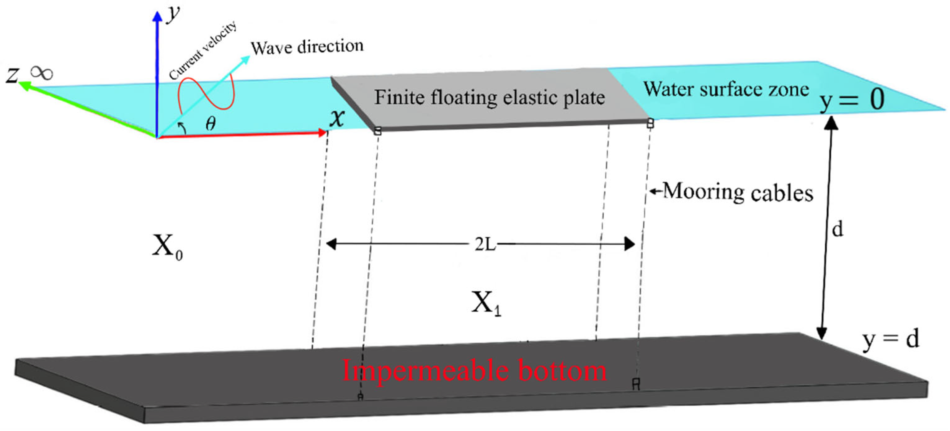
The model setting of this case is viewed using a 3D Cartesian coordinate system where the plane $x-z$ is horizontal and the positive y-axis points downwards. In this framework, a finite FEP is placed at the free surface $y=0$ over water of FD $y=d$ with infinitley extended $z-$direction. Therefore, the whole fluid zone can be designed as: $-\infty <x<-L, 0<y<h,-\infty <z<\infty$ and $L<x<\infty , 0<y<h,-\infty <z<\infty$ denoted by ${\mathsf{X}}_0$ whilst, $-L<x<L, 0<y<h,-\infty <z<\infty$ refer to ${\mathsf{X}}_1$ with edges of the FEP at $x=-L$ and $x=L$ (as shown in Figure 2). It is assumed that the incident wave travels at an angle of $\theta$ ($0<\theta <\pi /2$) to the x-axis and an uniform following current is moving parallel to $z-$axis at a constant speed of $v_2=v$, and forms a right angle to the $x$-axis. Therefore, in the entire fluid regions, the total velocity potential $\psi (\overline{x};t)$ including the current condition is expressed as:

$$\psi \left(\overline{x};t\right)=vz+Re\left\{\phi \right(x,y\left)e^{i({\gamma }_{z}z-\omega t)}\right\},$$

(13)

where $\phi (x,y)$ is the spatial component of the velocity potential and Re is the real part of the compelx velocity potential in all the zones with ${\gamma }_z$, the wavenumber in the z direction, is defined as $k_{0}sin\theta$ with angular frequency $\omega$ and $k_0$ representing the wavenumber associated with the incident wave in open water zone, respectively. Thus, the three-dimensional Laplace equation was turned into a reduced wave equation and $\phi (x,y)$ fulfil the reduced wave equation,

$$({\partial }_{xx}+{\partial }_{yy}-{\gamma }_z^2)\phi =0, \mathrm{in} \mathrm{the} \mathrm{fluid} \mathrm{domain}$$

(14)

and the corresponding free surface elevation and FEP deflection of the form $\zeta \left(x,z,t\right)=Re\left\{\zeta \right(x\left)e^{i({\gamma }_{z}z-\omega t)}\right\}$ with $\zeta \left(x\right)$ satisfy the linearized kinematic and dynamic conditions near at $y=0$ as:

$${\phi }_y=-i(\omega -v{\gamma }_z)\zeta (x)$$

(15)

$$\zeta (x)=-(i/g)(\omega -v{\gamma }_z)\phi$$

(16)

By combining conditions (15) and (16) and eliminating $\zeta (x)$, the free surface condition as follows:

$${\phi }_{0y}=\left(-1/g\right){(\omega -v{\gamma }_z)}^2{\phi }_0$$

(17)

Whilst the dynamic linearized plate covered condition combined with CV and oblique angle can be expressed as:

$$\left\{EI{({\partial }_{xx}-{\gamma }_z^2)}^2+\mathbb{C}\left({\partial }_{xx}-{\gamma }_z^2\right)-{\rho }_{p}d{\omega }^2+\rho g\right\}\zeta =(-i\rho )(\omega -v{\gamma }_z){\phi }_1.$$

(18)

Combining Equations (15) and (18), one can derive the plate-covered boundary condition in the presence of CV and oblique angle as:

$$\{K{({\partial }_{xx}-{\gamma }_z^2)}^2+\Theta ({\partial }_{xx}-{\gamma }_z^2)-{\chi }_p{\omega }^2+1\}{\phi }_{1y}=(-1/g){(\omega -v{\gamma }_z)}^2{\phi }_1, x\in \left[-L,L\right], z\in \left(-\infty ,\infty \right),$$

(19)

The symbols used in Equation (19) are the same as in Equation (6) and ${\chi }_p={\rho }_{p}d/\rho g$.

On the impermeable bottom at $y=d$ (FD) and $y\to \infty$ (ID), the spatial velocity potential satisfies the following condition as:

$${\phi }_y=0 \mathrm{and} \phi , \left|\nabla \phi \right|\to 0$$

(20)

The moored edge conditions at $x=\pm L$ on $z\in (-\infty ,\infty )$ with cable stiffness $k_j$, yield:

$$\left\{EI\left({\partial }_{xx}-v{\gamma }_z^2\right)\right\}{\varphi }_y=0$$

(21a)

$$\left\{EI\left({\partial }_{xx}-(2-\upsilon ){\gamma }_z^2\right){\partial }_x+\mathbb{C}{\partial }_x\right\}{\varphi }_y=k_j{\partial }_y\varphi ,$$

(21b)

Finally, the far field condition associated with the oblique wave and CV as follows:

$$\phi \left(x,y\right)=\left(I_0{e}^{-i\sqrt{{(k}_0^2-{\gamma }_z^2)}x}+R_0{e}^{i\sqrt{{(k}_0^2-{\gamma }_z^2)}x}\right)g_0(v,y) \mathrm{a}\mathrm{s} x\to \infty$$

(22a)

$$\phi \left(x,y\right)=T_0{e}^{-i\sqrt{{(k}_0^2-{\gamma }_z^2)}x}{g}_0\left(v,y\right) \mathrm{a}\mathrm{s} x\to -\infty .$$

(22b)

where $g_0\left(v,y\right)={\displaystyle \frac{ig}{\left(\omega -v{\gamma }_z\right)}}{\displaystyle \frac{cosh{k}_0(d-y)}{cosh{k}_{0}d}}$ and $k_0$ satisfy the dispersion relation as defined below Equation (12).

It may be noted that while the 3D and oblique wave formulation can handle both following and opposing wave-current conditions, the presented results focus on following currents to avoid wave blocking, a phenomenon that can occur when waves encounter opposing currents.

The next subsection will derive the Green’s function associated with the formulation developed in Section 3 in both the cases of FD and ID using the fundamental source potential function under oblique wave, with the current case, along with their DR.

Derivation of Green’s Function Under Oblique Wave and Current in FD and ID

It may be mentioned that previous work [31] investigated the hydroelastic response of a moored, floating plate using a BIEM formulation, in the absence of current velocity and without employing a series expansion-based derivation of the Green’s function.

In the context of the oblique wave case and CV, here, it is assumed that the Green’s function $\mathcal{G}(\overline{x};{\overline{\eta }}_0)$ with ${\overline{\eta }}_0=({\eta }_0,{\xi }_0)$ being the source point and $\overline{x}=(x,y)$ being any point in the fluid domain. Thus, $\mathcal{G}(\overline{x};{\overline{\eta }}_0)$ satisfies the reduced wave equation:

$$({\partial }_{xx}+{\partial }_{yy}-{\gamma }_z^2)\mathcal{G}=0\mathrm{except} \mathrm{at} {\overline{\eta }}_0,$$

(23)

along with the condition (23), BCs (4a,b), and near ${\overline{\eta }}_0$, $\mathcal{G}(\overline{x};{\overline{\eta }}_0)$ satisfy:

$$\mathcal{G}\approx K_0({\gamma }_{z}r), r=\sqrt{{(x-{\eta }_0)}^2+{(y-{\xi }_0)}^2}\to 0$$

(24)

where $K_0({\gamma }_{z}r)$ is the zeroth-order modified Bessel function of the second kind.

In FD, let ${\overline{\eta }}_0$ be in $-\infty <x<\infty , 0<y<d, 0<z<\infty$, $\mathcal{G}(\overline{x};{\overline{\eta }}_0)$ can be expanded by satisfying Equations (23), (4a), and (24) as:

$$\mathcal{G}(\overline{x};{\overline{\eta }}_0)=K_0\left({\gamma }_{z}r\right)-K_0\left({\gamma }_z{r}^{\prime }\right)+{\int }_0^{\infty }\tilde{A}(q,y)\mathit{cos}v(x-{\eta }_0)dq, 0<y<d,$$

(25)

where $r^{\prime }=\sqrt{{(x-{\eta }_0)}^2+{(2d-y-{\xi }_0)}^2}$, $\tilde{A}(q,y)=A(q)\mathit{cosh}qy+B(q)\mathit{sinh}qy$,

$$\begin{array}{l}A(q)={\displaystyle \frac{2q({\rm K}{q}^4+\Theta q^2+1)e^{-\sqrt{u^2+{\gamma }_z^2}(d-{\xi }_0)}}{qS(q)}}\\ +{\displaystyle \frac{e^{\sqrt{u^2+{\gamma }_z^2}{\xi }_0}}{S(q)q}}\left[\{({\rm K}{q}^4+\Theta q^2+1)-(1/g){(\omega -vq)}^2\}+e^{-2\sqrt{u^2+{\gamma }_z^2}d}\{({\rm K}{q}^4+\Theta q^2+1)+(1/g){(\omega -vq)}^2\}\right]\end{array}$$

$$B(q)={\displaystyle \frac{2e^{-\sqrt{u^2+{\gamma }_z^2}(d-{\xi }_0)}-qA(q)\sinh qd}{q\cosh qd}}$$

$$S(q)=q({\rm K}{q}^4+\Theta q^2+1)\tanh qd-(1/g){(\omega -vq)}^2$$

(26)

with $q=\sqrt{u^2+{\gamma }_z^2}$. Further, the values for $K_0({\gamma }_{z}r)$ and $K_0({\gamma }_z{r}^{\prime })$ in Equation (25) are the same as in [32]. It is worth mentioning that $S(q)=0$ in Equation (26) is the DR with a floating plate, oblique wave, and CV.

Utilizing the Cauchy residue theorem, considering the roots that ensure boundedness of the subsequent series expansion, and substituting the values of $K_0({\gamma }_{z}r)$ and $K_0({\gamma }_z{r}^{\prime })$, Equation (25) takes the expansion as:

$$\mathcal{G}(\overline{x};{\overline{\eta }}_0)={\displaystyle \sum _{n=0,I}^{II}{A}_n{g}_n(q_n,y)e^{i{u}_n\left|x-x_0\right|}+}{\displaystyle \sum _{n=1}^{\infty }{B}_n{F}_n({\mu }_n,y)e^{-\sqrt{{\mu }_n^2+{\gamma }_z^2}\left|x-x_0\right|}}$$

(27)

where $g_n(q_n,y)={\displaystyle \frac{\cosh q_n(d-y)}{\cosh q_{n}d}}$, with $q_n^2=u_n^2+{\gamma }_z^2$ and the unknown $A_n$’s are obtained as $A_n={\displaystyle \frac{i\pi \cosh q_n(d-{\xi }_0)}{q_n{M}_n}} \mathrm{for} 0<{\xi }_0<d$ with $M_n={\displaystyle \frac{S^{\prime }(q_n)}{2({\rm K}{q}^4+\Theta q^2+1)}}$, and $B_n$ in Equation (27) can be obtained by putting $u_n=i{\mu }_n$ in the expression $A_n$ with the superscript ‘dash’ in $S(q_n)$ indicates the partial derivative w.r.t. $q_n$.

Similarly, in case of ID, when ${\overline{\eta }}_0=({\eta }_0,{\xi }_0)$ is in $0<y<\infty$, $\mathcal{G}(\overline{x};{\overline{\eta }}_0)$ can be takes the following form by satisfying Equations (23), (16) and (4b) as:

$$\mathcal{G}(\overline{x};{\overline{\eta }}_0)=K_0({\gamma }_{z}r)-K_0({\gamma }_z{r}^{\prime })+{\displaystyle \underset{0}{\overset{\infty }{\int }}C(q)e^{-q(y-d)}\cos q(x-{\eta }_0)dq}, 0<y<\infty ,$$

(28)

where:

$$C(q)=-{\displaystyle \frac{e^{-\sqrt{k^2+{\gamma }_z^2}{\xi }_0}}{q}}\left[1-{\displaystyle \frac{e^{-2\sqrt{k^2+{\gamma }_z^2}d}\left\{q({\rm K}{q}^4+\Theta q^2+1)+(1/g){(\omega -qv)}^2\right\}}{S(q)}}\right]$$

(29)

with $S(q)=q({\rm K}{q}^4+\Theta q^2+1)-(1/g){(\omega -qv)}^2$ is the DR in FD.

The Green’s function in ID has an equivalent form that can be expanded as

$$\mathcal{G}(\overline{x};{\overline{\eta }}_0)={\displaystyle \sum _{n=0,I}^{II}{A}_n}{g}_n(q_n,y)e^{i{u}_n\left|x-{\eta }_0\right|}+{\displaystyle \underset{0}{\overset{\infty }{\int }}A(\tau )}\Upsilon (\tau ,y)e^{-\sqrt{{\zeta }^2+{\gamma }_z^2}\left|x-{\eta }_0\right|}d\tau$$

(30)

with:

$$g_n(y)=e^{-q_{n}y} \mathrm{for} 0<y<\infty$$

$$\mathsf{\gamma }(\tau ,y)=\tau ({\rm K}{\tau }^4+\Theta {\tau }^2+1)\cos \tau y-(1/g){(\omega -v\tau )}^2\sin \tau y,$$

$${\rm N}(\tau ,y)=-(\tau \sin \tau d+(1/g){(\omega -v\tau )}^2\cos \tau d)(1/g){(\omega -v\tau )}^2$$

$$A_n={\displaystyle \frac{-i\pi e^{-q_n({\xi }_0-2d)}}{q_n{\Omega }_n}} \mathrm{for} 0<{\xi }_0<\infty$$

$$A(\tau )={\displaystyle \frac{-\{(1/g){(\omega -v\tau )}^2(\tau \cos \tau {\xi }_0-(1/g){(\omega -v\tau )}^2\sin \tau {\xi }_0)-{\rm N}(\tau )\cos \tau ({\xi }_0-d)\}}{\pi \sqrt{{\tau }^2+{\gamma }_z^2}\Delta (\tau )}}, 0<{\xi }_0<\infty ,$$

$$\Delta (\tau )={{\rm N}}^2(\tau )+2{\rm N}(\tau )L_1(\tau ,h)+({\tau }^2+{\{(1/g){(\omega -qv)}^2\}}^2){\{(1/g){(\omega -qv)}^2\}}^2$$

$${\Omega }_n={\displaystyle \frac{S^{\prime }(q_n)}{2({\rm K}{q}_n^4+\Theta q_n^2+1)}}$$

Next, we will present a comparative analysis between the phase velocity $U_p$ and group velocity $U_g$ for different oblique wave angles with a particular value of CV in FD.

In FD, the expressions for the phase velocity $U_p$ and group velocity $U_g$ from Equation (22) in the presence of oblique incidence angle and CV can be derived as.

$$U_p=v\pm {\left[g\left\{K{(v^2-{\gamma }_z^2)}^{3/2}+\Theta {(v^2-{\gamma }_z^2)}^{1/2}+\left(1/{(v^2-{\gamma }_z^2)}^{1/2}\right)\right\}tanh\left({(v^2-{\gamma }_z^2)}^{1/2}\right)d\right]}^{1/2}$$

(31)

$$U_g=U_p+v(1-ϵ)$$

(32)

where $\epsilon ={\displaystyle \frac{1}{2}}\left\{{\displaystyle \frac{2u_{n}d}{sinh2u_{n}d}}+{\displaystyle \frac{\left(5K{u}_n^4-3\Theta u_n^2+1\right)}{(K{u}_n^4-\Theta u_n^2+1)}}\right\}$.

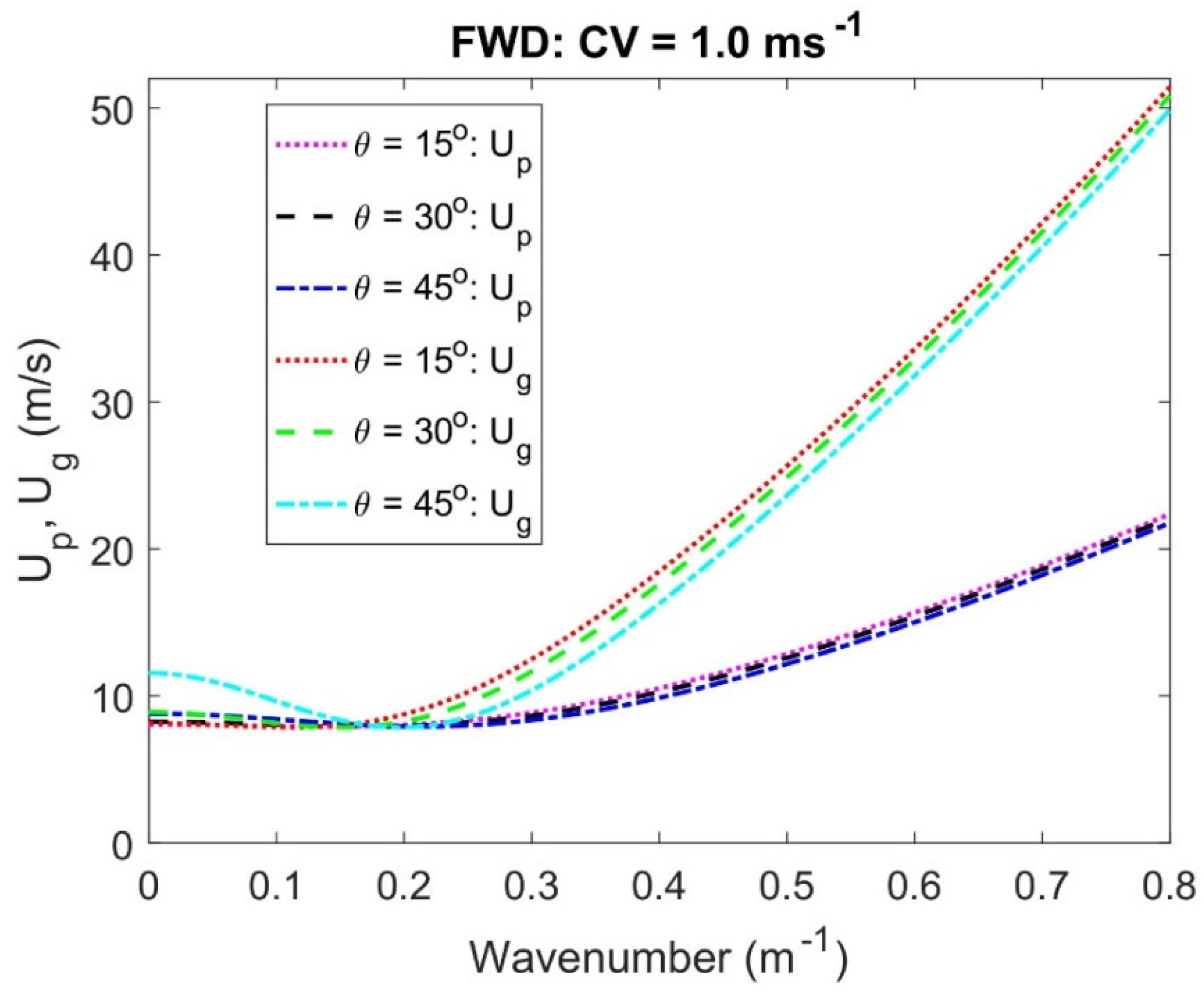
Figure 3 demonstrates the effect of various $\theta$ with a certain value of CV for the comparison of $U_p$ and $U_g$ vs. wavenumber in FD. In general, the observations are similar in both cases for different values of oblique angle $\theta$ increases, the values of $U_p$ and $U_g$ become lower. However, the group velocity travels faster than the phase velocity. This is because the group of waves, along with CV pushes significantly in the upstream region, which leads to faster waves.

Further, in the case of group velocity, wave energy propagates at a group speed different from the phase velocity, influenced by incidence angles, a specific CV value, and compressive force across the FEP. This group speed represents the movement of the wave energy, while phase velocity describes the movement of individual wave crests. This phenomenon is attributed to a higher group velocity than that of the phase velocity. However, this variation is negligible (almost they merge) at a particular value of wavenumber, which may be due to the change of phase.

Hereafter, the Green’s function, DR, phase velocity, group velocity, comparative analysis, and velocity decomposition method in the framework of geometrical symmetry of the 3D BVP will be presented and analyzed.

4. 3D Green’s Function and Plate Covered Zone DR

Recently, a Green’s function associated with a floating horizontal flexible membrane in 3D with wave-current interaction was derived in different water depths (see [7]). It is assumed that the fluid properties and structural behavior remain consistent with those defined in Section 2. This section presents the DR derived from the FEP scenario, considering current conditions in both FD and ID, which derivation is accomplished by utilizing Green’s function approach that takes into account fundamental source potentials.

Further, it is assumed that $\mathcal{G}(\overline{y};\overline{\tau })$ denotes the spatial component of 3D Green’s function with the source point $\overline{\tau }=({\tau }_1,{\tau }_2,{\tau }_3)$ and $\overline{y}=(x,y,z)$ represents any position within the fluid zone, usually known as Green’s function. Hence, $\mathcal{G}(\overline{y};\overline{\tau })$ satisfies the 3D Laplace equation:

$$({\partial }_{xx}+{\partial }_{yy}+{\partial }_{zz})\mathcal{G}=0\mathrm{except} \mathrm{at} (\overline{\tau }),$$

(33)

along with the floating plate condition (6) and the bottom boundary conditions (4a,b). Further, near the source point $(\overline{\tau })$, Green’s function $\mathcal{G}(\overline{y};\overline{\tau })$ satisfies

$$\mathcal{G}\approx {\displaystyle \frac{1}{\upsilon }},$$

(34)

as $\upsilon =\sqrt{{(x-{\tau }_1)}^2+{(y-{\tau }_2)}^2+{(z-{\tau }_3)}^2}\to 0$. In the case of water of FD, let the source point $(\overline{\tau })$ be in between the FEP and the sea bottom with the consideration of $x\in (-\infty ,\infty ), y\in (0,d), z\in \left[0,l\right]$, Green’s function $\mathcal{G}(\overline{y};\overline{\tau })$ satisfying Equation (26), along with the FD boundary condition (4a) and (34) is obtained as:

$$\mathcal{G}(\overline{y};\overline{\tau })={\displaystyle \frac{1}{2\pi }}{\displaystyle \underset{-\pi }{\overset{\pi }{\int }}{\displaystyle \underset{0}{\overset{\infty }{\int }}\left[e^{-q\left|y-{\tau }_2\right|}+e^{-q\left|2h-y-{\tau }_2\right|}\right.}}\left.+\{A(q)\coth qy+B(q)\}\sinh (qy)\right]\Lambda (q,\alpha )dqd\alpha ,$$

(35)

The first two terms of the integral account for the original source and its mirrored image with respect to the lower boundary. $(1/\upsilon )+(1/{\upsilon }_d)$ with ${\upsilon }_d=\sqrt{{(x-{\tau }_1)}^2+{(2d-{\tau }_2-y)}^2+{(z-{\tau }_3)}^2}$ and $\Lambda (q,\alpha )=\exp [iq\{(x-{\tau }_1)\cos \alpha +(z-{\tau }_3)\sin \alpha \}]$.

By using (6) and the Riemann-Lebesgue lemma, it is feasible to find the unknowns $A(q) \mathrm{and} B(q)$ associated with Equation (35) as follows:

$$\left.\begin{array}{l}A(q)={\displaystyle \frac{-2\exp (-qd)\cosh q(d-{\tau }_2)\{(1/g){(\omega -vq)}^2+q({\rm K}{q}^4+\Theta q^2+1)\}}{\Delta (q)}},\\ B(q)={\displaystyle \frac{2\exp (-qd)\cosh q(d-{\tau }_2)\{(1/g){(\omega -vq)}^2+q({\rm K}{q}^4+\Theta q^2+1)\}}{\Delta (q)}}\tanh qd\end{array}\right\}$$

(36)

where:

$$\Delta (q)=(1/g){(\omega -vq)}^2-q({\rm K}{q}^4+\Theta q^2+1)\tanh qd.$$

(37)

The DR (37) allied to gravity wave interaction with the FEP under the current conditions has one real root $q_0$, four complex roots $q_I,q_{II},q_{III},q_{IV}$, and an infinite number of purely imaginary roots $q_n, n=1,2,\dots ,$. The roots of the DR (37) are determined by employing the iterative numerical technique known as the Newton–Raphson method for real roots. Additionally, contour plots can be utilized to derive initial estimates for locating the complex roots of DR (37).

In a similar manner, when the source $(\overline{\tau })$ is located in water of ID, and $-\infty <x<\infty$ $0<y<\infty$, and $0<z<l$, the Green’s function $\mathcal{G}(\overline{y};\overline{\tau })$ that satisfies the 3D Laplace equation, along with the infinite bottom BC (4b), (33) and (34), can be expressed as:

$$\mathcal{G}(\overline{y};\overline{\tau })={\displaystyle \frac{1}{2\pi }}{\displaystyle \underset{-\pi }{\overset{\pi }{\int }}{\displaystyle \underset{0}{\overset{\infty }{\int }}\left[e^{-q\left|y-{\tau }_2\right|}+e^{-q\left|2d-y-{\tau }_2\right|}\right.}}\left.+C(p)e^{-qy}\right]\Lambda (q,\alpha )dqd\alpha ,y\in (0,\infty ),$$

(38)

with $\Lambda (q,\alpha )$ is identical to Equation (36).

By applying the BC (6), the constants $C(p)$ in the Expression (38) can be determined as:

$$C(q)={\displaystyle \frac{-2\exp (-qd)\cosh q(d-{\tau }_2)\{(1/g){(\omega -vq)}^2+q({\rm K}{q}^4+\Theta q^2+1)\}}{\Delta (q)}}$$

(39)

where:

$$\Delta (q)=(1/g){(\omega -vq)}^2-q({\rm K}{q}^4+\Theta q^2+1)$$

(40)

with $\Delta (q)=0$ is the DR in the water of ID.

It can be checked that if we set the flexural rigidity ${\rm K}=0$, $q=p$, $d=h$, $v=u,$ and $\Theta =\sigma$ in DRs (37) and (40), then the reduced DRs will be the same as in Equations (28) and (33), respectively, as found previously [7].

It can be mentioned that the integral form of 3D Green’s functions (35) and (38) can be simplified using the Cauchy integral theorem based on complex function theory to obtain an alternative series expression; this approach could aid in demonstrating a realistic physical behavior for problems in ocean engineering.

The next subsection will analyse the wave propagation rate, such as phase velocity ($U_p$) and group velocity $\left(U_g\right)$ for different current velocities along with structural parameters in different cases.

Comparative Analysis and Effect of Current Velocity on the Phase Velocity and Group Velocity

The analytical expressions in the presence of $v$ for the $U_p$ and $U_g$ can be obtained from the DR as defined in Equation (37) in water of FD as.

For FD water, the $U_p$ and $U_g$ can derived as:

$$U_p=v\pm {\left[g\{K{q}^3+\Theta q+(1/q)\}\tanh qd\right]}^{1/2}, U_g=U_p\mathcal{F}+v(1-\mathcal{F}),$$

(41)

where $\mathcal{F}=\left\{{\displaystyle \frac{q_{n}d}{2\sinh 2q_{n}d}}+{\displaystyle \frac{(5K{q}_n^4+3\Theta q_n^2+1)}{2(K{q}_n^4+\Theta q_n^2+1)}}\right\}$.

Similarly, in the case of deep and shallow water depths by considering the assumption $\mathrm{t}\mathrm{a}\mathrm{n}\mathrm{h}qd\approx 1$ and $\mathrm{t}\mathrm{a}\mathrm{n}\mathrm{h}qd\approx qd$ one can easily derive the $U_p$ and $U_g$.

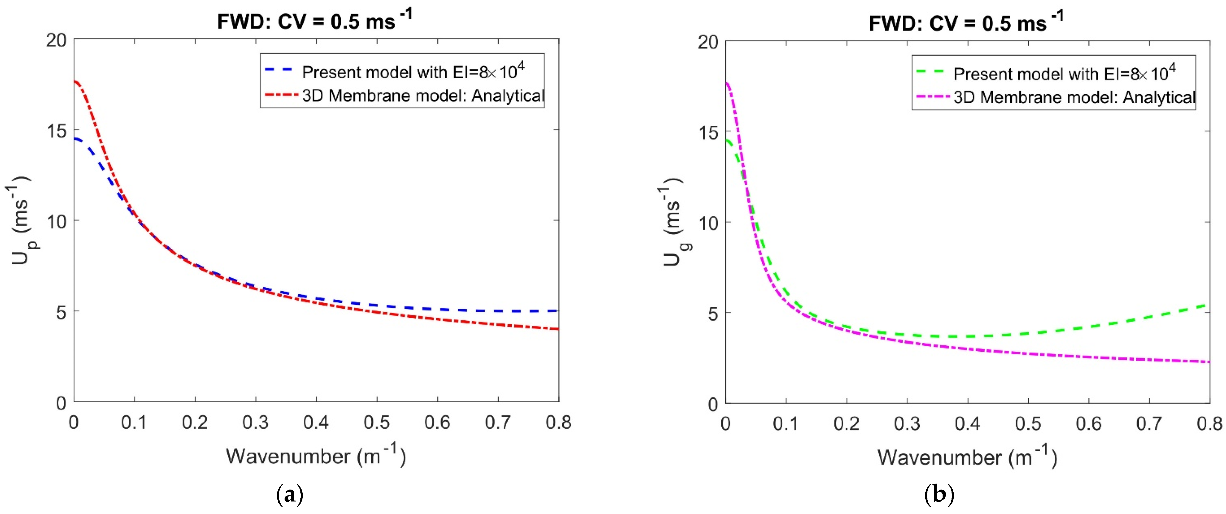
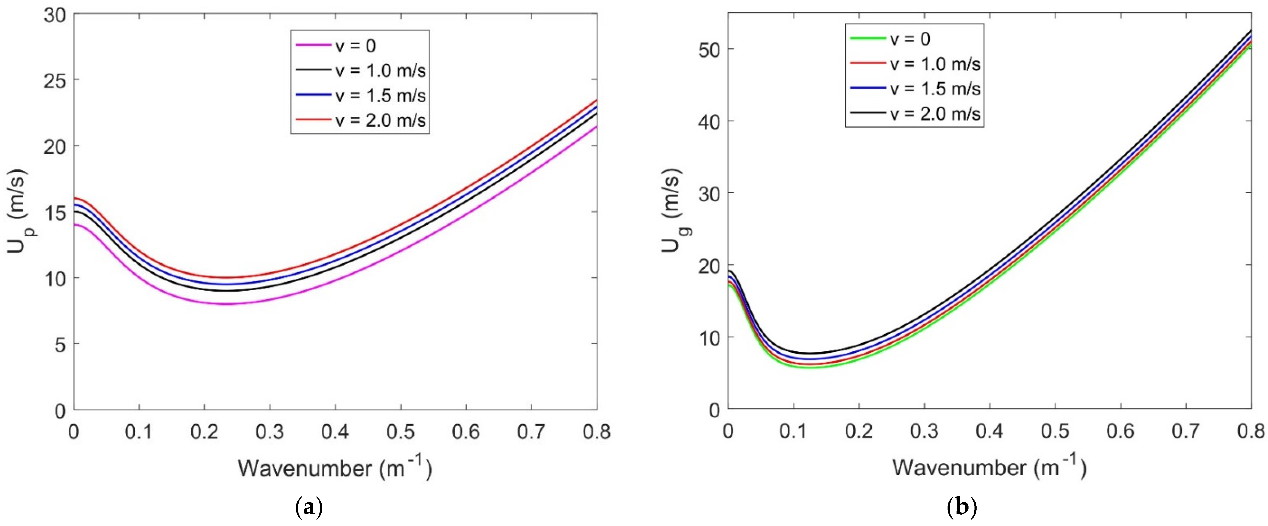
In Figure 4a,b, a comparative result of $U_p$ and $U_g$ between the present model and the result obtained by [7] without flexural rigidity versus wavenumber with other parameters are mentioned in the Figure caption. It is found that for smaller values of wavenumber, the present $U_p$ and $U_g$ moves a lower speed than that of [7], whilst, for higher wavenumber this trend becomes reversed. This lowering role of the present model results is due to the presence of flexural rigidity that prevents higher flexibility than that of membrane model, which leads to smaller values in $U_p$ and $U_g$. However, although the peak values for both cases are the same, a significant difference is observed as the wave number increases. Moreover, in both Figures, $U_p$ and $U_g$ from the model [7] are 17.538, while the present model is 14.418 m, which is 20.8% lower.

Figure 5 compares the $U_p$ and $U_g$ of waves over the FEP vs. wavenumber with $v=1.5 \mathrm{m}/\mathrm{s}$. From Figure 5a, in FD, it is found that as the CV increases the values $U_p$ become higher but the trend is increasing in nature for larger wavenumbers. While, for $U_g$ (Figure 5b) the general observations are similar to that of Figure 5a but the peak values are higher than that of $U_p$. However for lower wavenumbers, the $U_g$ moves faster than those of $U_p$. The observed effect stems from the non-evanescent propagation of waves across the FEP and, for the case of no CV, both $U_p$ and $U_g$ have smaller values than those of any one of the CV values.

The upcoming subsection will establish the DR related to the 3D specified problem using Green’s function technique, and this derived relation will be applied in the subsequent subsections.

5. Velocity Decomposition Method in 3D in the Framework of Geometrical Symmetry of the BVP

The initial BVP demonstrates geometric symmetry, allowing it to be divided into two straightforward semi-infinite BVPs. These problems are formulated in the semi-infinite zone along the x-axis and can be solved with $x\in (0,x)$ relative ease.

To formulate the system of linear equations, we utilize the orthogonal relationship linked to the eigenfunctions in ${{\rm X}}_o$. Therefore, for our objectives, it suffices to examine the region $x\in (0,\infty )$, $z\in \left[0,l\right]$, as the solution can be extrapolated across the entire domain through symmetric relationships. Following the same approach as in [30,33], the divided potentials ${\mathbb{Z}}_1\left(\overline{y}\right)$ and ${\mathbb{Z}}_2\left(\overline{y}\right)$ can be represented as a symmetric potential, ${\varphi }_{\mathrm{SP}}(x,\overline{z})$, $x>0$, and an anti-symmetric potential, ${\varphi }_{\mathrm{AP}}(-x,\overline{z})$, $x<0$, for z ∈ [0, l] as:

$$\left.\begin{array}{c}{\mathbb{Z}}_1\left(\overline{y}\right)={\varphi }_{\mathrm{SP}}(x,\overline{z})-{\varphi }_{\mathrm{AP}}(-x,\overline{z})\\ {\mathbb{Z}}_2\left(\overline{y}\right)={\varphi }_{\mathrm{SP}}(x,\overline{z})+{\varphi }_{\mathrm{AP}}(-x,\overline{z})\end{array}\right\}$$

(42)

The expressions ${\mathbb{Z}}_1\left(\overline{y}\right)$ and ${\mathbb{Z}}_2\left(\overline{y}\right)$ are obtained by applying the Fourier expansion formulas, ensuring that they fulfill Equations (2), (3), (4a) and (6) as follows:

$${\mathbb{Z}}_1(\overline{y})=\left\{\begin{array}{c}{\sum }_m\left\{\mathcal{l}(v,k_0)A_{m0}{e}^{-i{\alpha }_{m0}(x-L)}{{\rm M}}_{m0}\left(\overline{z}\right)\right.\left.-{\sum }_n\mathcal{l}(v,k_n)a_{mn}{e}^{i{\alpha }_{mn}(x-L)}{{\rm M}}_{mn}\left(\overline{z}\right)\right\}, x\in (L,\infty ),\\ {\sum }_m{\sum }_n\mathcal{l}(v,q_n)c_{mn}{\chi }_{mn}^A\left(x\right){\Omega }_{mn}\left(\overline{z}\right),x\in (0,L),\end{array}\right.$$

(43)

$${\mathbb{Z}}_2(\overline{y})=\left\{\begin{array}{c}{\sum }_m\mathcal{l}(v,k_0)\left\{A_{m0}{e}^{-i{\alpha }_{m0}(x-L)}{{\rm M}}_{m0}\left(\overline{z}\right)\right.-\left.{\sum }_n\mathcal{l}(v,k_n)b_{mn}{e}^{i{\alpha }_{mn}(x-L)}{{\rm M}}_{mn}\left(\overline{z}\right)\right\}, x\in (L,\infty ),\\ {\sum }_m{\sum }_n\mathcal{l}(v,q_n){\overline{c}}_{mn}{\chi }_{mn}^S\left(x\right){\Omega }_{mn}\left(\overline{z}\right), x\in (0,L)\end{array}\right.,$$

(44)

where ${\alpha }_{mn}^2=k_n^2-{\beta }_m^2$ for $n=0,I,II,III,IV,1,\dots$ and $m=0,1,2,\dots$. $\mathcal{l}(v,k_n)=g/2i(\omega -v{k}_n)$.

Further, the symmetric and anti-symmetric functions are the same as in [28] with $q_{mn}^2=q_n^2-{\beta }_m^2$ and $a_{mn}, b_{mn}{, \mathrm{c}}_{\mathrm{mn}}$, and ${\overline{\mathrm{c}}}_{\mathrm{mn}}$ are the unknowns to be determined. The eigenfunction ${\Omega }_{mn}(\overline{z})$ and the normalized vertical eigenfunction ${{\rm M}}_{mn}(\overline{z})$ are being the same as in [28], hence, ${{\rm M}}_{mn}(\overline{z})$ satisfy the orthogonal relation $\langle {{\rm M}}_{mn}(\overline{z}), {{\rm M}}_{jl}(\overline{z})\rangle =(l/2){\delta }_{mj}{\delta }_{nl}$ with ${\delta }_{mj} \mathrm{and} {\delta }_{nl}$ are the Kronecker delta.

The moored edge condition (8) on $z\in \left[0,l\right]$ in terms of the divided potential as:

$$EI\left({\partial }_x^2+\upsilon {\partial }_z^2\right){\mathbb{Z}}_{1y}(L,0,z)=0$$

(45a)

$${\partial }_x\left\{EI\left({\partial }_x^2+(2-\upsilon ){\partial }_z^2\right)+ℂ\right\}{\mathbb{Z}}_{2y}(L,0,z)=k_f{\mathbb{Z}}_{2xy}(L,0,z)$$

(45b)

where $k_1=k_2=k_f$. The side wall conditions for $x\in (-L,L)$ by the divided potential as:

$$EI\left({\partial }_x^2+\upsilon {\partial }_z^2\right){\mathbb{Z}}_{1y}(x,0,l)=0$$

(46)

$${\partial }_x\left\{EI\left({\partial }_x^2+(2-\upsilon ){\partial }_z^2\right)+ℂ\right\}{\mathbb{Z}}_{2y}(x,0,l)=0$$

(47)

The continuity conditions (9–10) over $0\le z\le l$ give:

$${\mathbb{Z}}_{1y}(0,0)=0,{\mathbb{Z}}_{2xy}(0,0)=0$$

(48)

The continuity of pressure and velocity at the interface at $x=L$ for $z\in \left[0,l\right]$ in Equation (11a,b) yield:

$${\mathbb{Z}}_1\left(\overline{y}\right)=0, {\mathbb{Z}}_{2x}\left(\overline{y}\right)=0.$$

(49)

Ultimately, the far-field radiation condition is expressed in the following form:

$${\mathbb{Z}}_1\left(\overline{y}\right)\approx {\sum }_{m=0}^{\infty }\left(A_{m0}{e}^{-i{\lambda }_{m0}x}+u_{m0}{e}^{i{\lambda }_{m0}x}\right){{\rm M}}_{m0}\left(\overline{z}\right), x\to \infty$$

(50)

$${\mathbb{Z}}_2\left(\overline{y}\right)\approx {\sum }_{m=0}^{\infty }\left(A_{m0}{e}^{-i{\lambda }_{m0}x}+v_{m0}{e}^{i{\lambda }_{m0}x}\right){{\rm M}}_{m0}\left(\overline{z}\right), x\to -\infty$$

(51)

where $u_{m0}={\Re }_{m0}-{{\rm T}}_{m0}$ and $v_{m0}={\Re }_{m0}+{{\rm T}}_{m0}$.

The procedure for the determination of unknown coefficients $a_{mn}$, $c_{mn}$, $b_{mn}$, and ${\overline{c}}_{mn}$ Equations (43) and (44) are presented in Appendix A.

After identifying the unknown constants, the amplitudes of the reflection and transmission waves $u_{m0}$ and $v_{m0}$ can be determined. Subsequently, the respective formulas can evaluate the reflection coefficient $K_{rm}$ and transmission coefficient $K_{tm}$.

$$K_{rm}=\left|(u_{m0}+v_{m0})/2A_{m0}\right|$$

(52)

$$K_{tm}=\left|(u_{m0}-v_{m0})/2A_{m0}\right|$$

(53)

The non-dimensional vertical wave force exerted on the FEP is determined as follows:

$$F_m={\displaystyle \frac{i\omega }{2gL}}{\displaystyle \underset{0}{\overset{l}{\int }}{\displaystyle \underset{0}{\overset{L}{\int }}{\partial }_y{\left.({\mathbb{Z}}_1+{\mathbb{Z}}_2)\right|}_{y=0}dxdz}}$$

(54)

6. Quantitative Findings and Analysis

This Section compares the reflection and transmission coefficients calculated from the current analytical solutions with the results obtained by [31], in the absence of CV. The results of the reflection coefficients, displacements, and vertical wave force on the FEP for the impact of CV analyzed, and then the phase and group velocities on the effect of different CVs, are also studied.

Hereafter, all numerical computations are executed based on an analytical solution by considering fluid density $\rho =1025{ \mathrm{kgm}}^{-3}$, and acceleration due to gravity $g=9.8{ \mathrm{ms}}^{-2}$, $k_f={10}^6 \mathrm{N}{\mathrm{m}}^{-1}$, and the series is shortened to $N=25$ as it converges for $N=25$ unless stated otherwise. Further, the flexural rigidity $EI=4\times {10}^6 \mathrm{N}.{\mathrm{m}}^2$ in which for the practical case the wood type material could be used for FEP. Computations are performed using MATLAB R2022b, 64-bit (win64), and all numerical calculations derived from the analytical solution were executed on a desktop computer equipped with an Intel^® Core i7-4790 CPU operating at 3.60 GHz and 16 GB of RAM. On average, simulating each case takes approximately 5 to 8 min.

6.1. Validation Findings and Their Implications

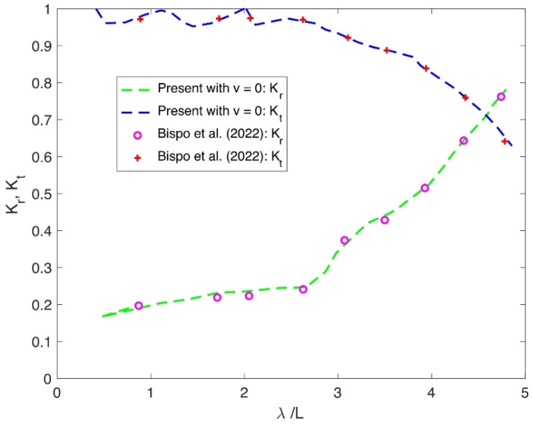
Here, the current analytical results for reflection and transmission coefficients $K_r$ and $K_t$ are validated to the theoretical model results obtained from [34] as shown in Figure 5 to assess the accuracy level. In Figure 6, the comparison between the reflection and transmission coefficients computed by the present results without CV and the theoretical results from [34] with $k_f={10}^6 \mathrm{N}{\mathrm{m}}^{-1}$, $L=69 \mathrm{m}, \mathrm{a}\mathrm{n}\mathrm{d} l=5 \mathrm{m}$ with higher flexural rigidity $EI={10}^9 \mathrm{N}{\mathrm{m}}^{-2}$ and compressive force $\mathbb{C}=\sqrt{EI\rho g}$ defined in the predicted model versus non-dimensional wavelength $\left(\lambda /L\right)$.

It is seen that the reflection and transmission coefficient patterns closely resemble those obtained by model [34] (as shown in Figure 6). The strong agreement between the data points indicates consistency between the two models. This similarity arises because the present model, when simplified by excluding CV, ($v=0)$, utilizes the same structural parameters as model [34] within the same theoretical framework. Thus, the present solution is supported by the existing results in the literature.

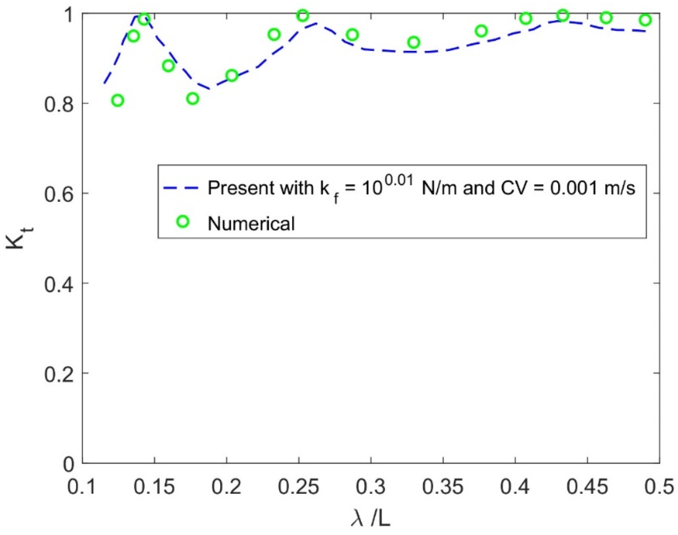
Figure 7 shows the comparison between the current result of $K_t$ with limiting case and result from the numerical Boundary Integral Equation Method obtained in [35] vs. $\lambda /L$ with elastic modulus $EI$ and water depth $h=50 \mathrm{m}$ with current speed $\mathrm{CV} =0.001 \mathrm{m}/\mathrm{s}$ and very small value of mooring stiffness $k_f={10}^{0.01} \mathrm{N}{\mathrm{m}}^{-1}$. A small value of $k_f$ and CV are chosen for a similar pattern between the results from [35] and the current model.

In Figure 7, the comparison confirms that the present model solution is consistent with the numerical model result. Nevertheless, the small differences can be discussed by the formulation under the consideration of CV and mooring lines of the current model, and these parameters were not assumed in the numerical model [35]. Further, the effect of flexural rigidity and mooring stiffness in the current model results in a lower $K_t$. In addition, in Figure 6, $K_t$ from the BIEM model is 0.993 m, while the current is 0.977 m, which is 1.7% larger.

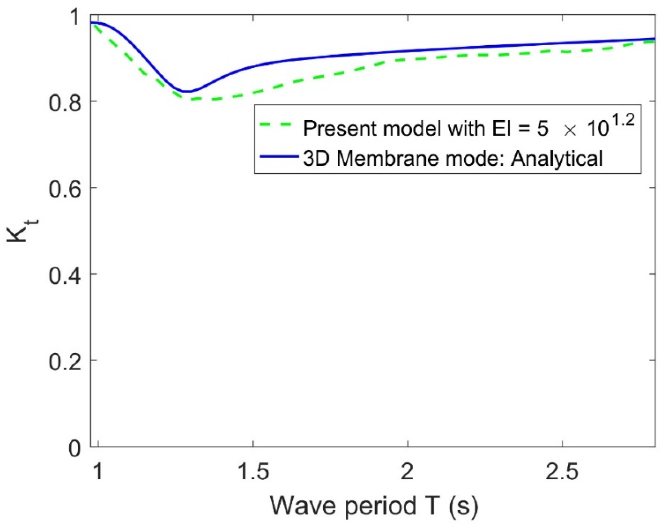
Figure 8 compares the present result of $K_t$ with the existing model result from the reference [7] versus wave period $T(\mathrm{s})$ with the other parametric values mentioned in Figure 8. It is observed that the transmission coefficient of the present result is lower than that of the result from the model [7] throughout the wave period. The observed difference stems from the flexural rigidity in the model, which causes greater reflection upstream and, consequently, reduced transmission downstream.

On the other hand, flexural rigidity enhances the structural rigidity, leading to a decrease in displacement and effectively mitigating deflection of the FEP compared to structures without this property. Further, in Figure 8, $K_t$ from [7] is 0.882 m, while the current model is 0.819 m, which is 7.7% larger.

6.2. Effect of Current and Structural Parameters on $K_{rm}$

Figure 9 plots the influence of $v$ on the $K_{rm}$ vs. non-dimensional wavelength $\lambda /L$ with modes of oscillation m = 1. An elevation in CV value corresponds to a heightened $K_{rm}$.

This is because the higher displacement of the FEP is caused by a higher CV, thereby enabling the transmission of greater wave energy beneath the plate. It is evident that in the absence of a current, no peak was observed in $K_{rm}$ (see [7]). Conversely, wave reflection attained zero minimum value (as shown in Figure 9) for certain intermediate non-dimensional wavenumbers, which may be due to phase change of incident and reflected waves leading to constructive/destructive interference of the waves in the combined effect of wave and current interactions. It was observed that the trend of $K_{tm}$ was almost the opposite pattern to that of $K_{rm}$ and hereafter, the results on $K_{tm}$ are deferred here.

Figure 10 presents the effect of the compressive force of the FEP on the $K_{rm}$ vs. $\lambda /L$. It is seen that the $K_{rm}$ rises as the values of the compressive force increase on the FEP. However, this influence becomes negligible for a smaller non-dimensional wavelength. Due to the FEP’s larger compressive strength, it exhibits lessened displacement, resulting in reduced wave energy transformation beneath the FEP and heightened wave reflection.

Figure 11 shows the $K_{rm}$ for different values of the flexural rigidity $EI$ versus the non-dimensional wavelength with other parametric values being the same as mentioned in the second paragraph of Section 6. The effects of flexural rigidity variation in the reflection coefficients presented in Figure 11 by comparison are visible, indicating that with a particular value of CV and mooring stiffness has noticeable influence on the studied coefficients, except for minimal wavelength values, where it can be seen in Figure 11, probably due to a reduction of energy loss by the mooring lines, since their stiffness is lower. On the other hand, the decrease in reflection coefficients at higher wavelengths, observed with increased flexural rigidity, suggests a correlation between higher flexural rigidity, reduced FEP flexibility, and increased reflection coefficients in the upstream region.

Figure 12 depicts the impact of different mooring stiffness on the $K_{rm}$ versus non-dimensional wavelength and being the same parametric values mentioned in the Figure caption. It is observed that by increasing the $k_f$, the $K_{rm}$ increases, which suggests that higher stiffness prevents the wave energy transformation, leading to lower reflection in the upstream region.

Figure 13 demonstrates the impact of the non-dimensional water depth $d/l$ on $K_{r1}$ versus $\lambda /L$ with l/d = 5, and L/d = 14. It is found that the $K_{rm}$ decreases with an increase in water depth. Which is because when the FEP is away from the seabed, a major part of the wave energy that is concentrated near the free surface is transmitted below the FEP as a result reflection coefficient at the upstream region getting reduced. This observation is similar to wave interaction with a submerged porous membrane as in [32].

Figure 14 presents the effect of the non-dimensional plate width $l/d$ on the reflection coefficient $K_{rm}$ versus $\lambda /L$ with $v=0.5 \mathrm{m}/\mathrm{s}$. Due to the increased plate coverage on the water plane, the $K_{rm}$ drops and reaches its lowest value for a wider structure. While the results for $K_{rm}$’s across various structural lengths are not depicted here, it is important to note that the observations are similar to those illustrated in Figure 13.

6.3. Influence of CV and Structural Parameters on Vertical Force

Figure 15 presents the impact of CV on the non-dimensional vertical wave force $F_m$ vs. $\lambda /L$ with $m=1$. As the values of CV increase, the $F_m$ on the FEP gets higher, which is due to the increase in fluid motion amplitude below the structure. Further, for an intermediate $\lambda /L$, the vertical wave load on the membrane increases with increasing CV. In addition, the effect of changing CV on water surface can be observed from this assessment that the higher CV has a more pronounced effect on the vertical force when compared to a lower CV. This effect is proportional, which means a higher CV has a higher hydrodynamic force that can significantly impact the vertical displacement of the structure.

Figure 16 shows the effect of membrane width on the non-dimensional $F_m$ with $v=0.5 m/s$ vs.$\lambda /L$. In general, the vertical wave load on the FEP lessens for a wider structure with a certain value of modes of oscillations, flexural rigidity, and CV. This is due to the fact that the FEP with a larger width has a larger projected area under a particular value of CV and mooring stiffness; at the same time, the elasticity properties of the FEP increase, which results in a larger hydrodynamic force that leads to higher vertical force on the structure.

In Figure 17, the influences of first three modes $m$ of the FEP on $F_m$ vs. $\lambda /L$ are plotted. It is observed that the $F_m$ rises with an increase in modes of oscillations $m$. The secondary modes of oscillation exhibit a sharp peak in $F_m$ at a smaller $\lambda /L$ and a higher value of $\lambda /L$ whilst tertiary oscillation modes reveal several distinct peaks, potentially inducing instabilities in the FEP displacement. This might be caused by the formation of small wave groups at the FEP edges, which dissipate before accumulating sufficient energy.

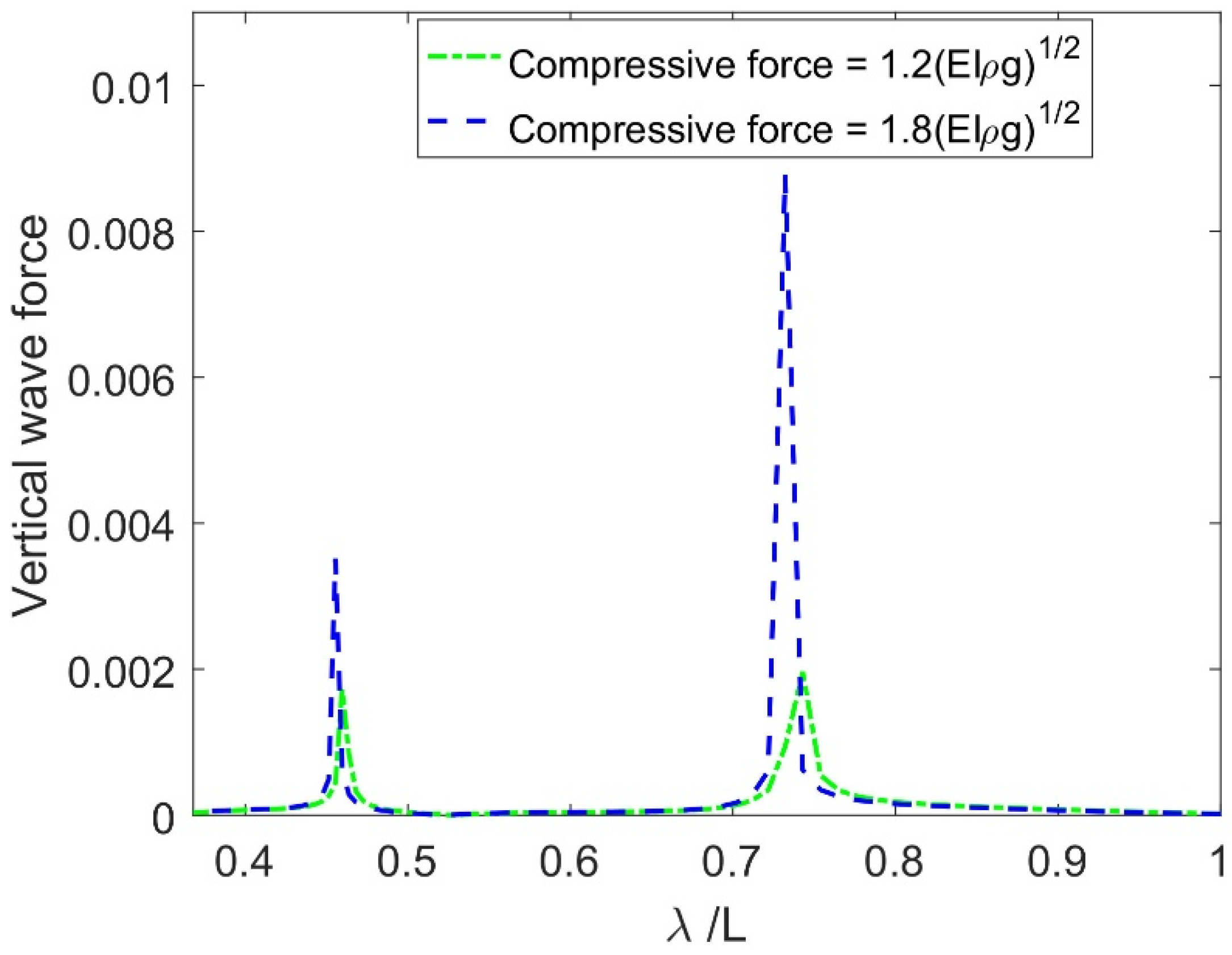
In Figure 18, the impacts of various $\mathbb{C}$ on $F_m$ vs. $\lambda /L$ are plotted. It is observed that the values of $F_m$ increases as the values of $\mathbb{C}$ becomes higher for certain values of mooring stiffness and $m=1$. However, for each value $\mathbb{C}$, the vertical load attends to a minimum because the membrane tension increases the flexibility of the FEP, as a result, the vertical force on the FEP increases.

NB: It may be noted that the sharp peaks observed in the vertical force in Figure 15, Figure 16 and Figure 18 are attributed to wave reflection: when waves strike the channel walls, a significant portion of their energy is reflected, and the collision of these reflected waves with the fluid inside the channel results in these peak forces.

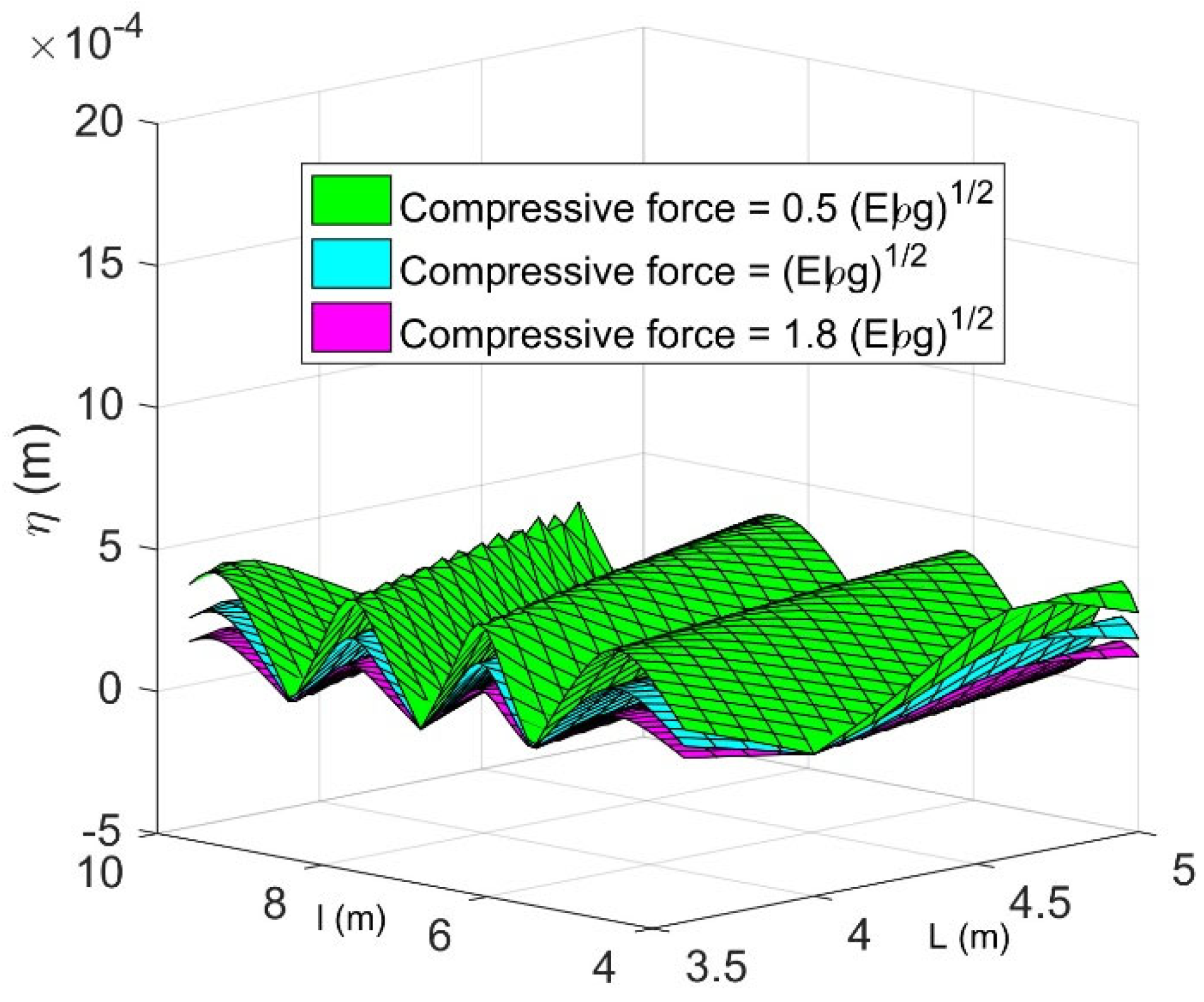
6.4. Impact of CV and Structural Parameters on 3D Displacement

Figure 19 simulates the 3D displacement $\eta (\mathrm{m})$ of the FEP for different CVs versus the length $L\left(m\right)$ and width $l\left(m\right)$ of the channel with compressive force $\mathbb{C}=\sqrt{EI\rho g} \mathrm{N}{\mathrm{m}}^{-1}$ with $v=1.5 \mathrm{m}/\mathrm{s}$. It is found that the displacement increases with an increase in the value of the CV. The larger displacement observed is a result of the hydrodynamic forces interacting with the given mooring stiffness and flexural rigidity of the FEP. 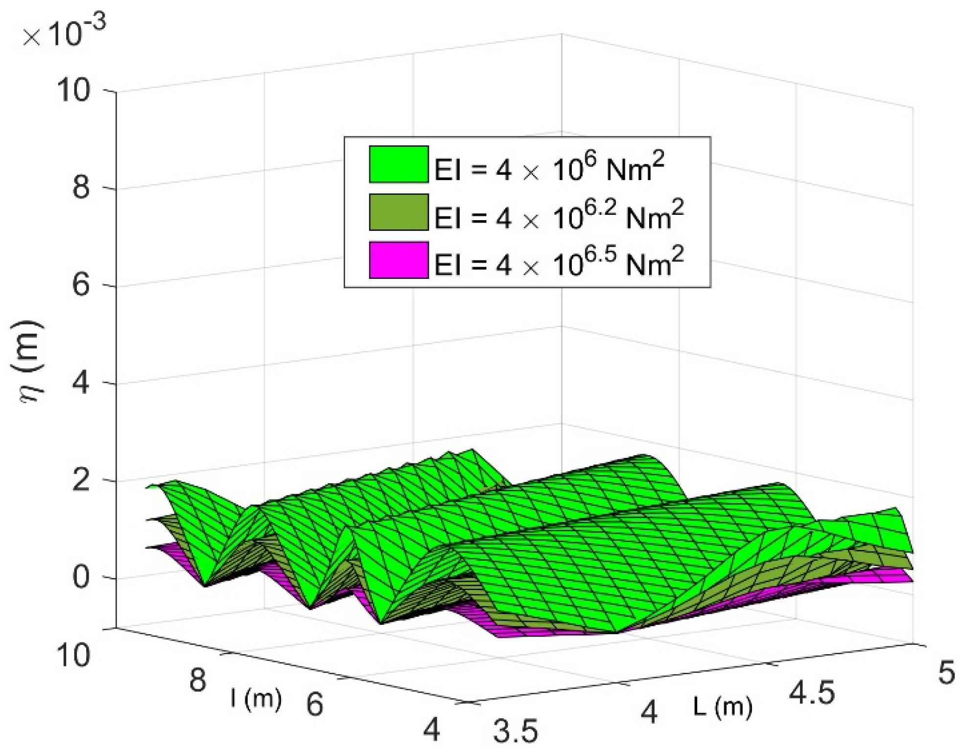However, for lower values of CV, the variations among them are negligible, which is clear from Figure 19.

Figure 20 simulates the 3D displacement $\eta (\mathrm{m})$ of the FEP for different flexural rigidity vs. the length $L\left(m\right)$ and width $l\left(m\right)$ of the channel with $\mathbb{C}=\sqrt{EI\rho g} \mathrm{N}{\mathrm{m}}^{-1}$ and $v=1.5 \mathrm{m}/\mathrm{s}$. An increase in $EI$ results in a decrease in displacement. This is due to the fact that the flexible structure becomes stiffer. Increased structural stiffness leads to a higher natural frequency, causing the structure to vibrate more rapidly. Moreover, flexural rigidity plays a role in determining the mode shapes of a structure. Greater flexural rigidity can produce more rigid mode shapes, characterized by reduced deformation during vibration. Typically, structures with higher flexural rigidity exhibit increased damping due to their enhanced resistance to deformation, leading to a decrease in the displacement.

Figure 21 plots the effect of different $\mathbb{C}$ on the 3D displacements of the FEP vs. $L\left(m\right)$ and width $l\left(m\right)$. It is seen that the observations are similar to those in Figure 20. However, in this case, the displacement variations for various $\mathbb{C}$ are significant. Moreover, as the compressive force increases, the wave force around the structure decreases, which leads to lower structural displacement. Further, with increase in the compressive force, the wavelength of the incident wave in the upstream region decreases, which lessens the structural displacement.

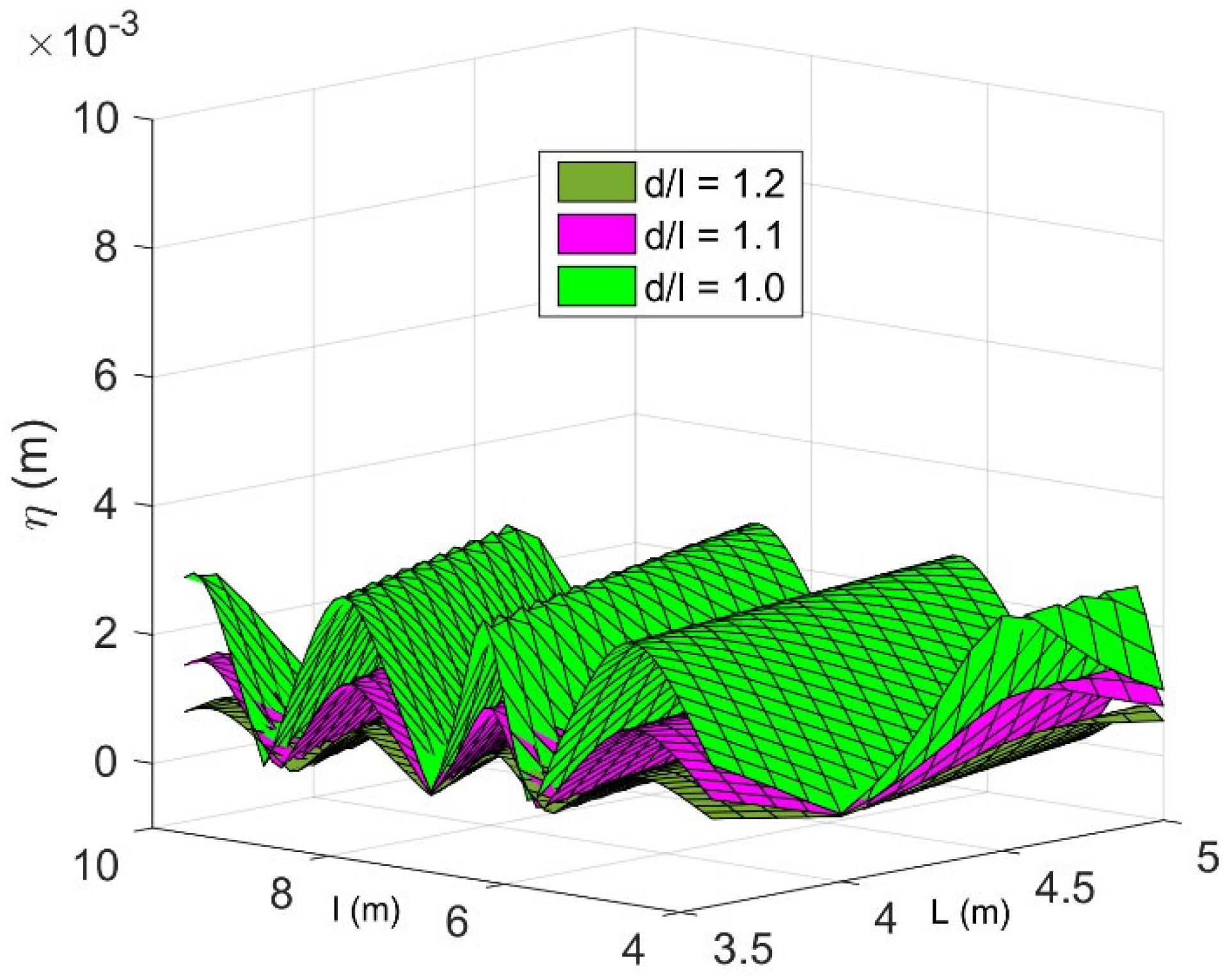
In Figure 22, the influence of various water depths $d/l$ on the 3D displacement of FEP vs. $L\left(m\right)$ and width $l\left(m\right)$ with $\mathbb{C}=\sqrt{EI\rho g} \mathrm{N}{\mathrm{m}}^{-1}$ are plotted. It is observed that the displacement becomes smaller for deeper water, which is due to the wave force on the FEP becoming lower as the $d/l$ rises. This phenomenon can be explained by the increased transmission of wave energy beneath the floating structure, leading to a reduction in wave force. Further, this occurs because a significant portion of wave energy is gradually absorbed while passing below the floating structure.

7. Conclusions

In this paper, the novel research contributions are the addition of CV to the 3D and oblique wave mathematical formulations, the derivation of Green’s function in series expansion form in FD and ID based on the reduced wave governing equation, and the comparative analysis of phase and group velocities in oblique wave and 3D cases. The comparisons between the limited case of the present results with previously published results are validated. Further, the effect of CV combined with design parameters on the hydroelastic response of a FEP is analysed in detail. It is concluded that:

The inclusion of current in the oblique wave mathematical formulation, derivation of Green’s function in series form using the Cauchy residue theorem in FD and ID, and comparative analysis of phase and group velocities for different oblique wave angles and in the 3D cases are the original contributions of this work. The comparison results indicated that the current results are supported by the existing hydroelastic numerical model, analytical model, and limiting cases of other calculations.

Comparative analysis indicates that (i) as the oblique angle increases for a particular value of CV, the phase and group velocities become lower, whilst both phase velocity and group velocity increase with increasing CV in the three-dimensional case, (ii) for lower value of wavenumber, the present phase and group velocities travel at a lower speed than that of existing 3D membrane model. However, group velocity exhibits higher peak values compared to the phase velocity, and at smaller wavenumbers, group velocity propagates faster.

It is observed that the reflection coefficients increase with higher CV, compressive force, and flexural rigidity, but decrease in deeper water. Vertical forces on the FEP are significantly affected by larger CV and higher modes of oscillation, whilst FEP displacement decreases with higher flexural rigidity and compressive force, but increases with CV.

In the future, the present model is to be generalized by utilizing a series of elastic linear dampers, which also function as wave energy absorbers. to increase the efficiency of wave energy extraction from the ocean waves emerging in the marine energy sectors.