The Mittag-Leffler–Caputo–Fabrizio Fractional Derivative and Its Numerical Approach

Abstract

This study introduces a novel fractional-order derivative, termed the Mittag-Leffler–Caputo–Fabrizio (MLCF) fractional derivative, which is characterized by a singular kernel. Symmetry plays a key role in the structure and behavior of fractional operators, and our formulation reflects this by incorporating symmetric properties of the Mittag-Leffler function and its integral representation. To numerically approximate the MLCF derivative, we apply a two-point finite forward difference scheme to estimate the first-order derivative of the function $u(\lambda )$ within the integral component of the definition. This leads to the construction of a new numerical differentiation scheme. Our analysis demonstrates that the proposed approximation exhibits first-order convergence, with absolute errors decreasing as the time step size h diminishes. These errors are quantified by comparing our numerical results with exact analytical solutions, reinforcing the accuracy of the method.

1. Introduction

Fractional derivatives extend the concept of classical differentiation by allowing the differentiation and integration of non-integer orders. Numerous definitions have been introduced in this field, including the $\psi$-Caputo–Katugampola derivative [1], the weighted Atangana–Baleanu fractional operators [2], the $\mathsf{\Theta }$-fractional operators [3], the $\psi$-proportional fractional operators [4], the $\psi$-weighted fractional operators [5], the $\psi$-Hilfer fractional operators [6], the $\phi$-conformable derivative [7], the nabla fractional operators [8], and the fractal fractional operators [9].

Differential equations involving arbitrary real orders $\nu >0$ serve as essential tools for modeling diverse physical systems across multiple disciplines, including science and engineering. Such equations find applications in areas such as statistical mechanics, Brownian motion, viscoelasticity, continuum and quantum mechanics, biosciences, chemical process engineering, and control systems. In [10], the authors studied the new mathematical model using the Caputo–Fabrizio fractional derivative. In [11], the authors studied the modeling of the dynamics of hepatitis E using the Caputo–Fabrizio derivative. More details on these applications can be found in [12,13,14,15,16,17,18,19,20,21] and related references.

The increasing attention toward fractional calculus (FC) has led to the emergence of multiple approaches for defining fractional integrals and derivatives. In contrast to the Riemann–Liouville fractional integral, derivatives have been formulated in numerous ways, with certain definitions equivalent only under specific conditions of the function being differentiated [22,23,24,25]. Furthermore, three recent classifications of fractional operators were explored in [26].

With the growing role of fractional derivatives in modeling complex physical phenomena, it becomes essential not only to establish a well-defined and widely accepted formulation for these derivatives but also to develop precise and efficient numerical approximations. This is particularly crucial for handling systems characterized by inherent singularities and nonlinearities [27,28,29,30,31]. However, the non-local nature of fractional operators poses challenges in designing computationally efficient algorithms, as they require incorporating all prior system states during simulations. This characteristic, often referred to as persistent memory, significantly increases both computational effort and processing time [32,33].

There are several numerical methods in the literature for Caputo–Fabrizio, such as finite difference methods, trapezoidal methods, and interpolation, among which we mention the two-point finite forward difference formula [34], Simpson’s $1/3$ rule [35], the quadratic interpolation-based $L1-2$ formula [36], and the $L1$ and $L1-2$ formulas using Lagrange interpolation [37].

To address this issue, various short-memory principles have been introduced in recent studies [38,39]. These approaches effectively reduce computational costs and minimize the accumulation of rounding errors when applying numerical methods, making them particularly advantageous for solving fractional initial value problems.

This study introduces a novel fractional derivative, referred to as the MLCF fractional derivative, along with a numerical scheme for its approximation. The proposed method utilizes a two-point finite difference approach to approximate the derivative term $u^{\prime }(\lambda )$. In addition, error analysis of this numerical approximation is presented. Consequently, this work formulates a numerical differentiation formula for the MLCF fractional derivative.

As demonstrated in Section 3, the error analysis reveals that the local truncation error of the proposed approximation contains a positive constant dependent on the fractional order $\nu$, resulting in an error term of $O(h)$. This confirms the first-order accuracy of the developed numerical approach. To enhance precision, the approximation is applied over a continuous temporal mesh, as elaborated in Section 4. Finally, Section 5 presents numerical experiments that validate the efficiency and accuracy of the proposed method.

2. Preliminaries

This section revisits fundamental definitions that are relevant to this study.

Definition 1

([12]). Let $0<\nu <1$. The Caputo fractional derivative for $u(\lambda )$ is defined as

$${}^{C}D_{\lambda }^{\nu }\left[u(\lambda )\right]={\displaystyle \frac{1}{\mathrm{\Gamma }(1-\nu )}}{\int }_0^{\lambda }{(\lambda -\tau )}^{-\nu }{u}^{\prime }(\tau )d\tau ,$$

(1)

where $\lambda >0,u\in C[0,\lambda ]$, with $\mathrm{\Gamma }(.)$ denoting the Gamma function.

Definition 2

([40]). Let $0<\nu <1$. The Caputo–Fabrizio derivative is expressed as follows:

$$\begin{array}{cc}\hfill {}^{CF}D_{\lambda }^{\nu }\left[u(\lambda )\right]& ={\displaystyle \frac{M(v)exp\left[-v\frac{\lambda }{1-\nu }\right]}{1-\nu }}{\int }_0^{\lambda }{u}^{\prime }(\tau )exp\left[\nu {\displaystyle \frac{\tau }{1-\nu }}\right]d\tau ,\hfill \end{array}$$

(2)

with $M(\nu )$ serving as a normalization function—any smoothness. $M(\nu )$ plays a role in the following:

1. 

Ensuring consistency at integer orders:

• When $\nu \to 0^{+}$, the fractional derivative should reduce to the original function $u(\lambda )$.
• When $\nu \to 1^{-}$, it should recover the classical first derivative $u^{\prime }(\lambda )$.
• Thus, $M(\nu )$ must satisfy

  $$M(0)=M(1)=1.$$

2. 

Dimensional analysis:

• The fractional derivative has units dependent on ν.
• $M(\nu )$ adjusts the operator so that both sides of the equation have consistent physical dimensions.

3. 

Kernel Normalization: The term ${\displaystyle \frac{M(\nu )}{1-\nu }}$ normalizes the exponential kernel to ensure proper weighting in the integral.

Additionally, u belongs to the Sobolev space $H^1(a,b)$ with $b>a$. It is worth noting that the given definition does not include a singular kernel. Definition 2 plays a central role in the forthcoming sections of this work.

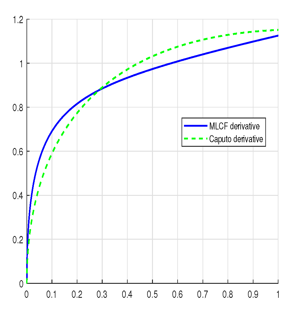
3. The Mittag-Leffler–Caputo–Fabrizio Fractional Derivative

In this section, we present the new fractional derivative termed the Mittag-Leffler–Caputo–Fabrizio fractional derivative. From the Definition 2, we have new definitions:

Definition 3.

Let $0<\nu <1$ and $0<\alpha \le 1$. The Mittag-Leffler–Caputo–Fabrizio fractional derivative is defined as follows:

$$\begin{array}{cc}\hfill {}^{MLCF}\mathcal{D}_{\lambda }^{\nu ,\alpha }u(\lambda )& ={\displaystyle \frac{M(\nu ){\mathbb{E}}_{\alpha }{(\frac{\nu }{1-\nu }{\lambda }^{\alpha })}^{-1}}{1-\nu }}{\int }_0^{\lambda }{\mathbb{E}}_{\alpha }({\displaystyle \frac{\nu }{1-\nu }}{s}^{\alpha })u^{\prime }(s)ds,\hfill \end{array}$$

(3)

where the one-parameter Mittag-Leffler function is

$${\mathbb{E}}_{\alpha }(\lambda )=\sum _{k=0}^{\infty }{\displaystyle \frac{{\lambda }^k}{\mathrm{\Gamma }(\alpha k+1)}}.$$

There are many uses for the Mittag-Leffler function; see [41,42,43,44,45,46].

Remark 1.

This definition is a generalization of the Caputo–Fabrizio derivative with the flexibility of α and ν. If $\alpha =1$, we obtain the Caputo–Fabrizio fractional derivative in Definition 2.

4. Numerical Approximation

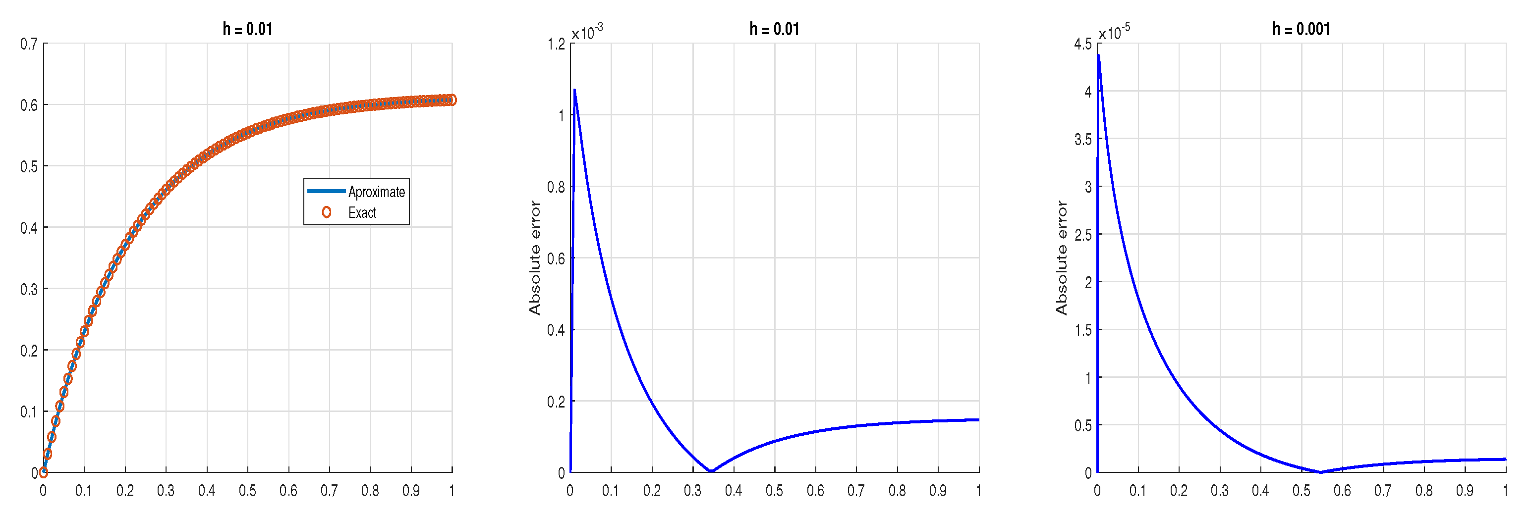
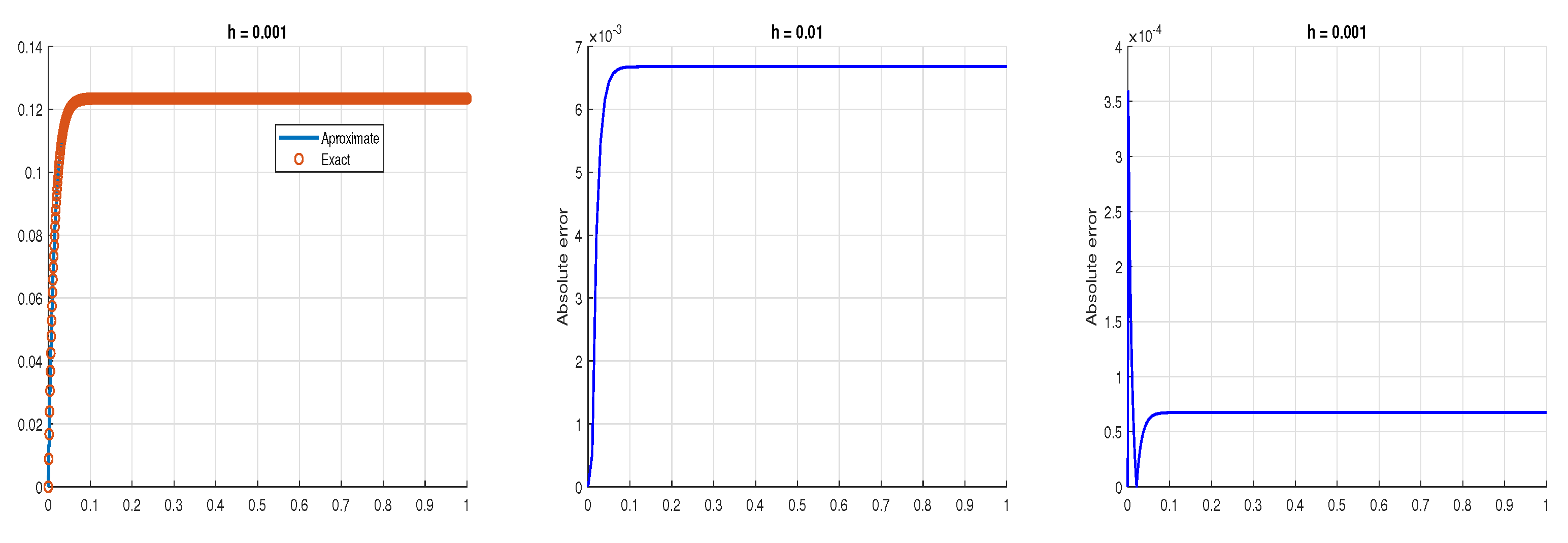
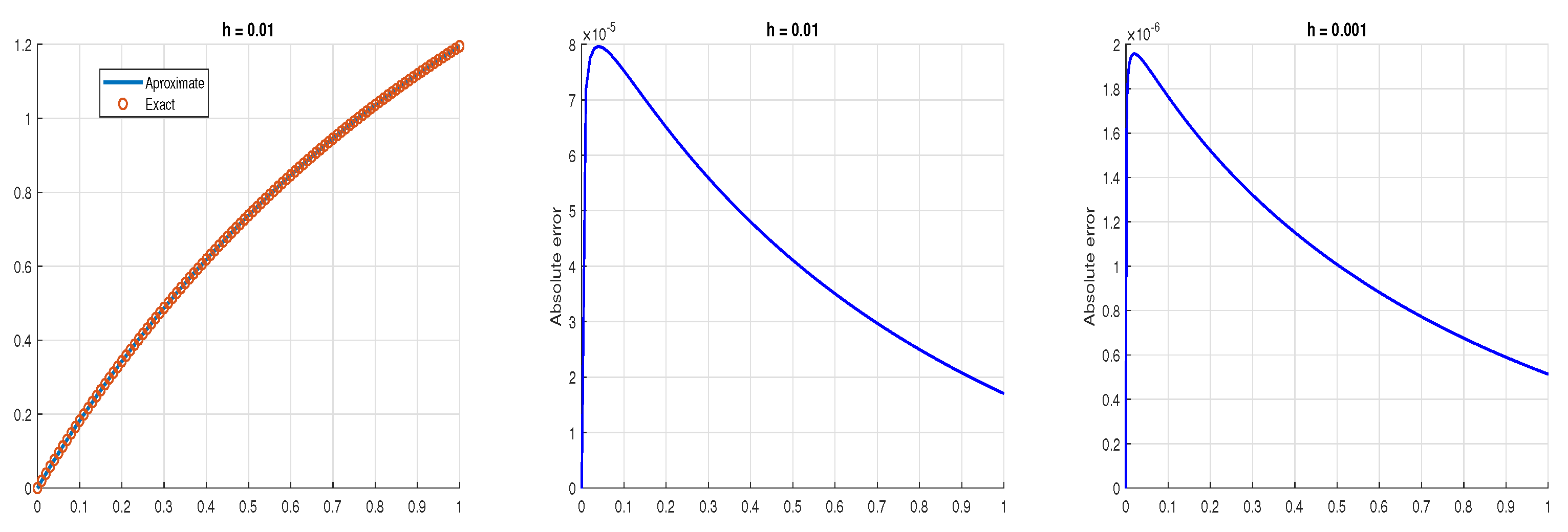
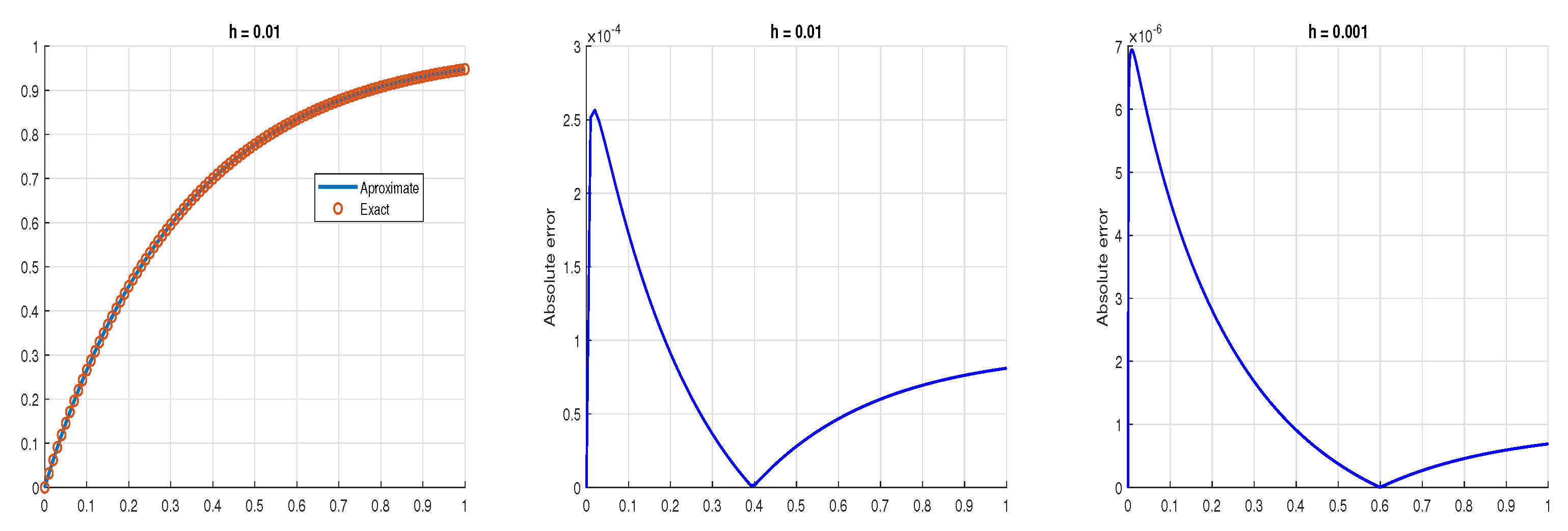
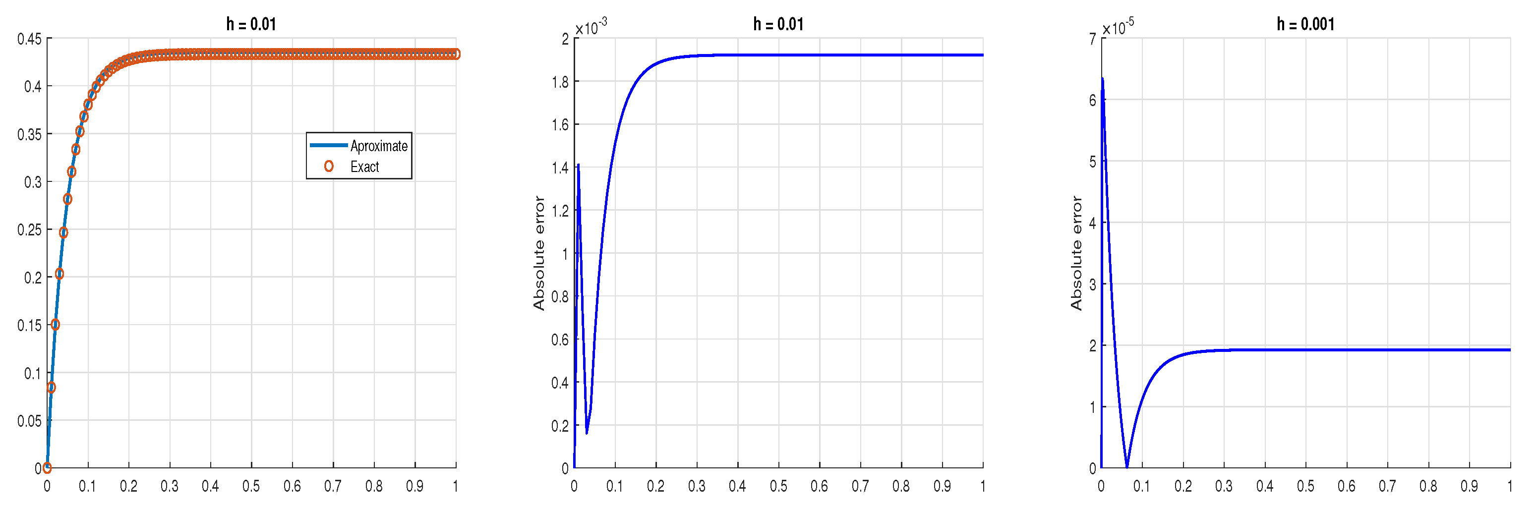
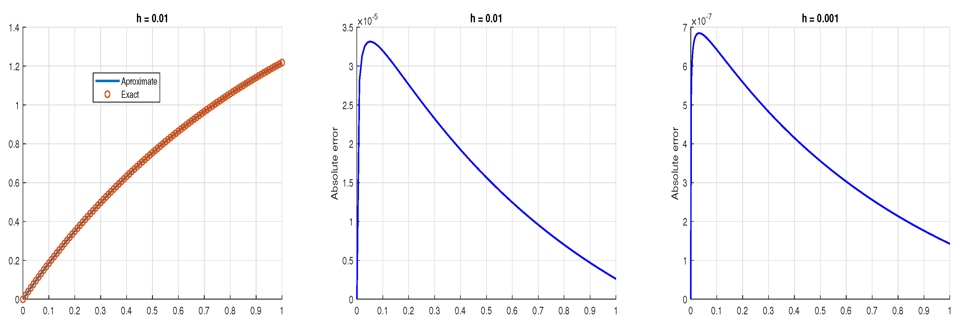
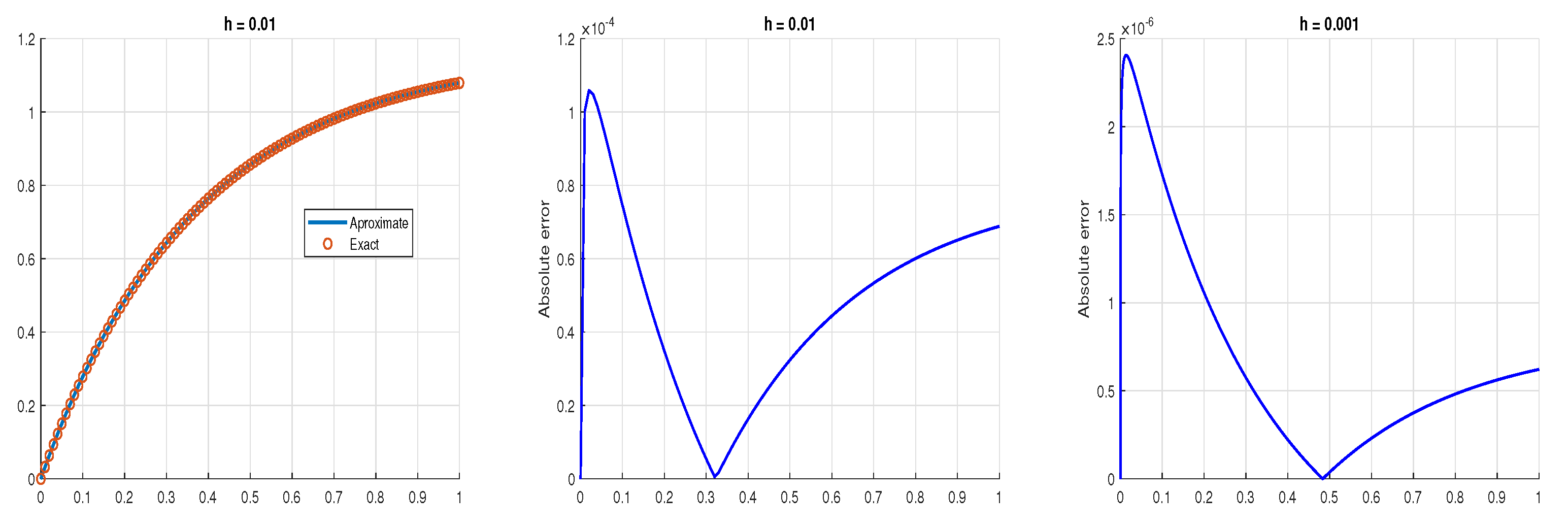
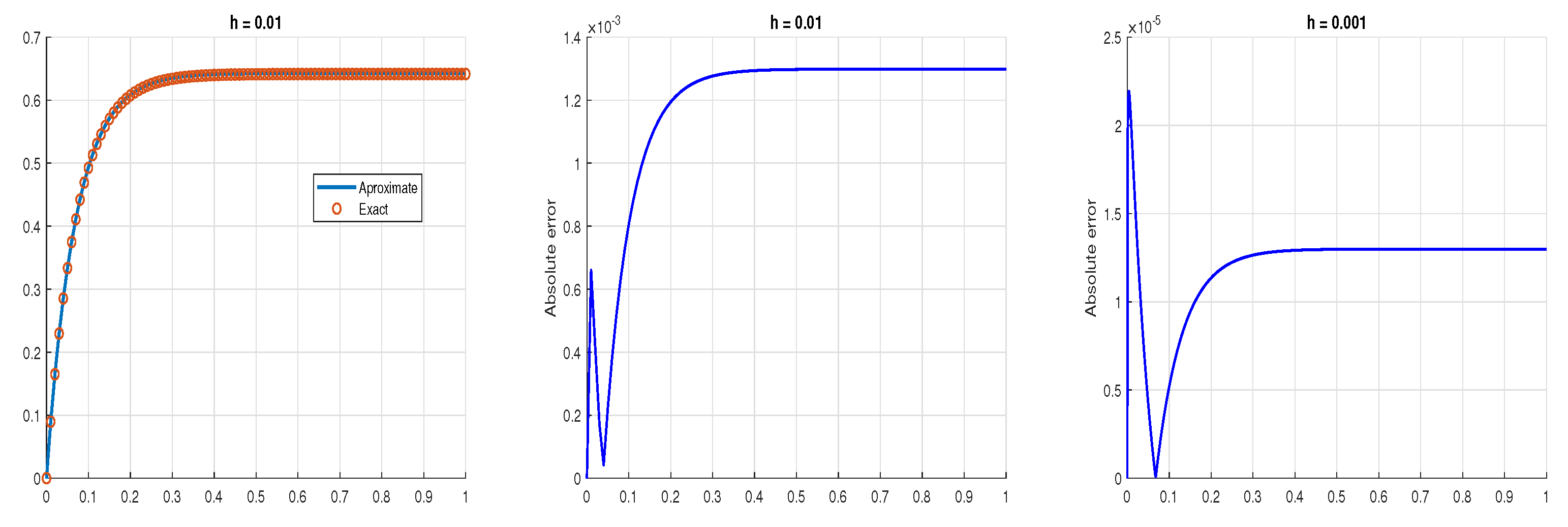
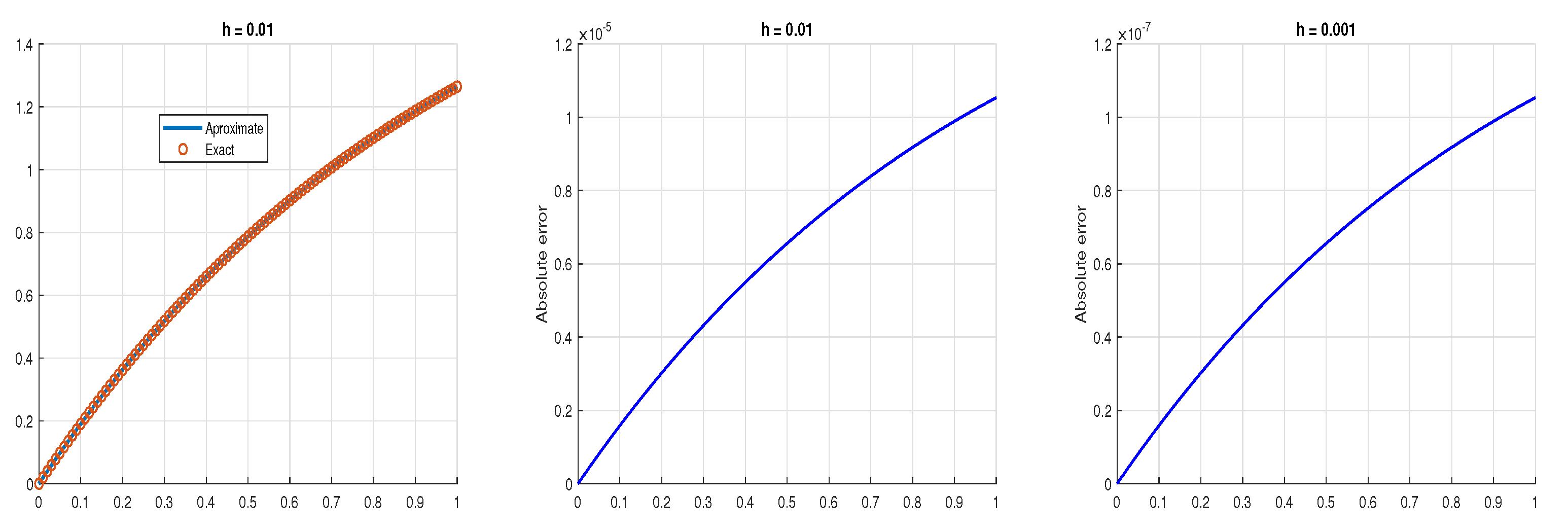
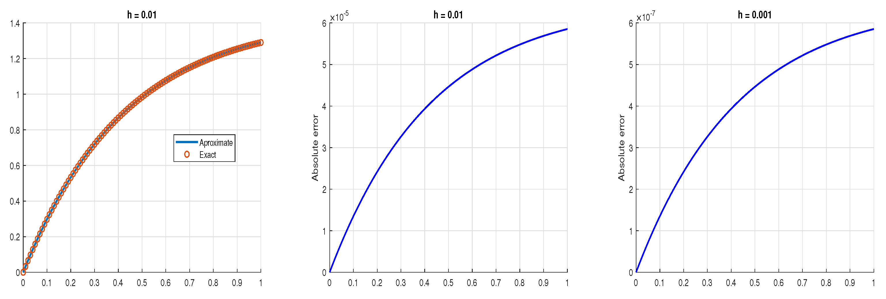
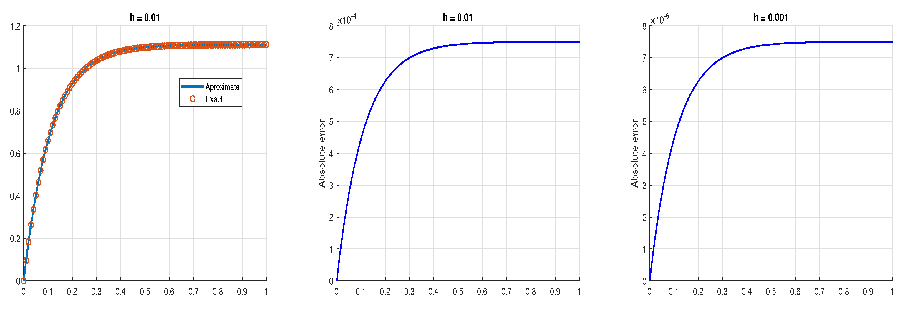
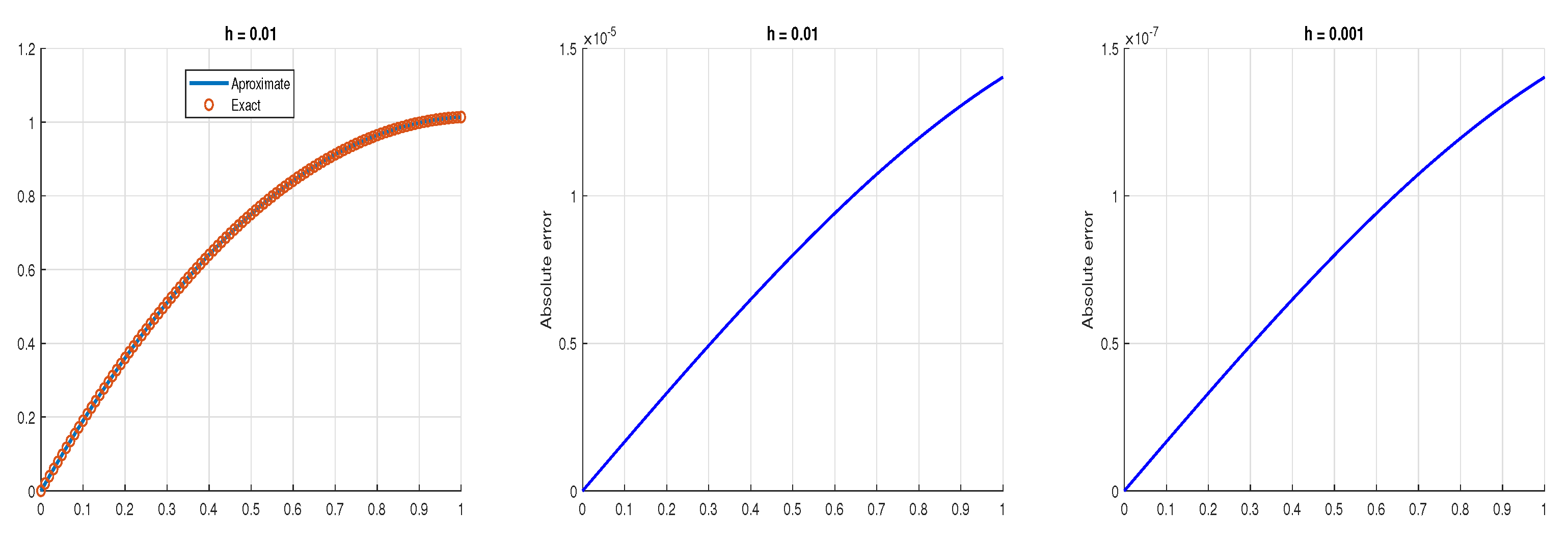
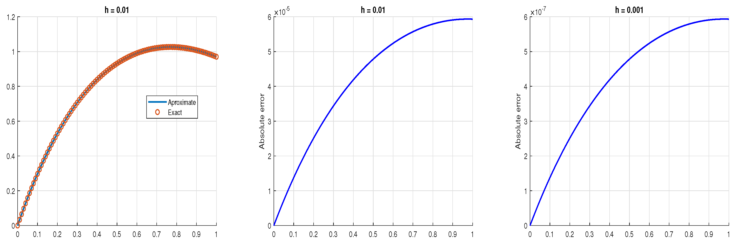
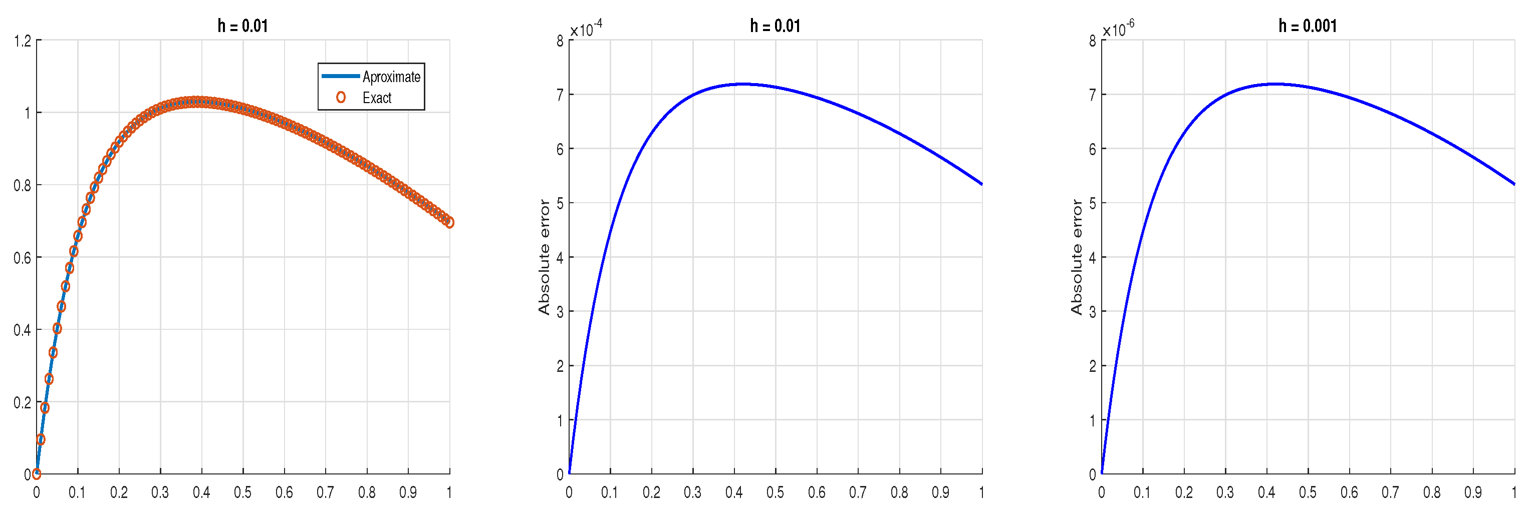
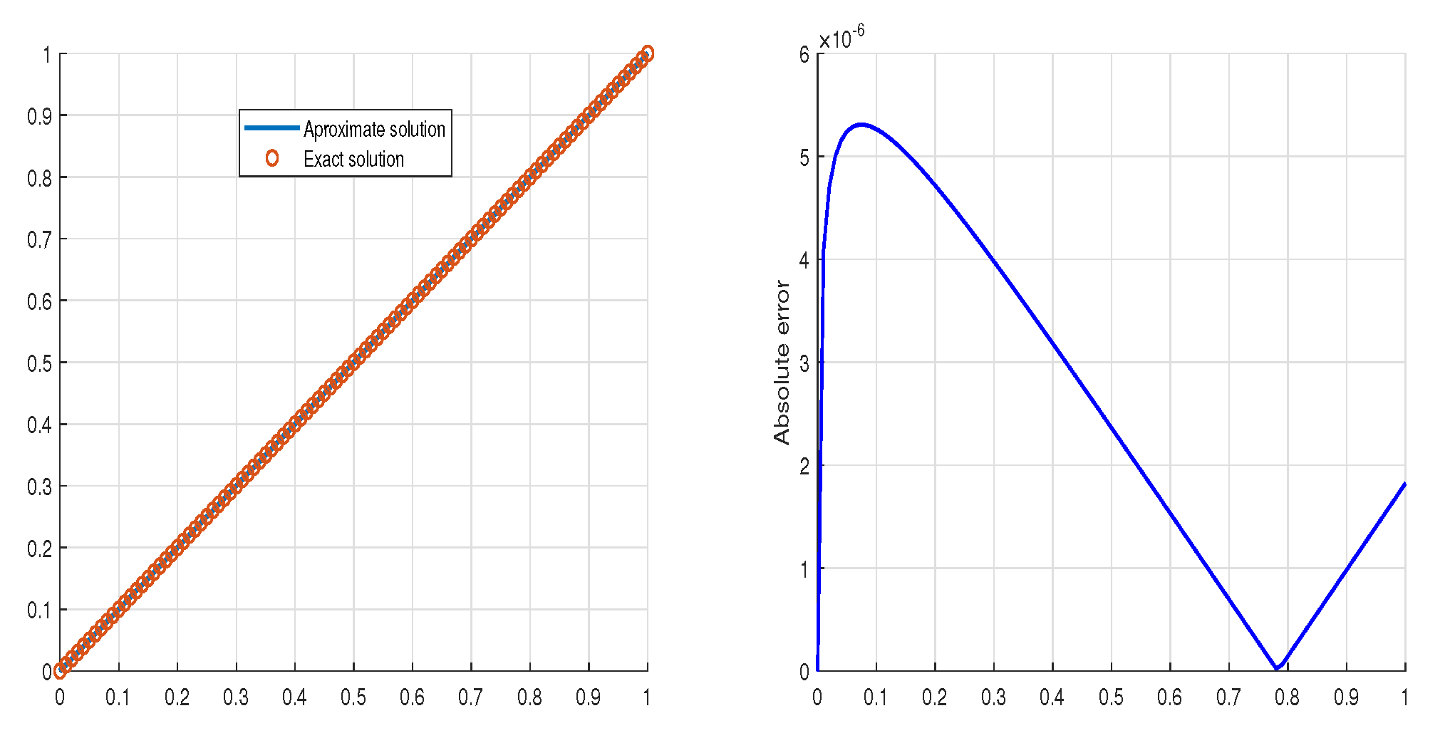
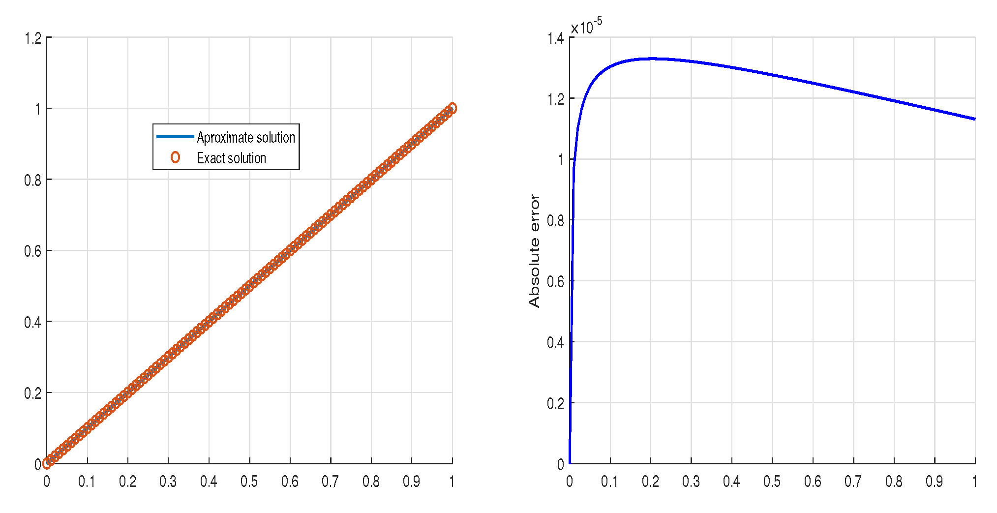
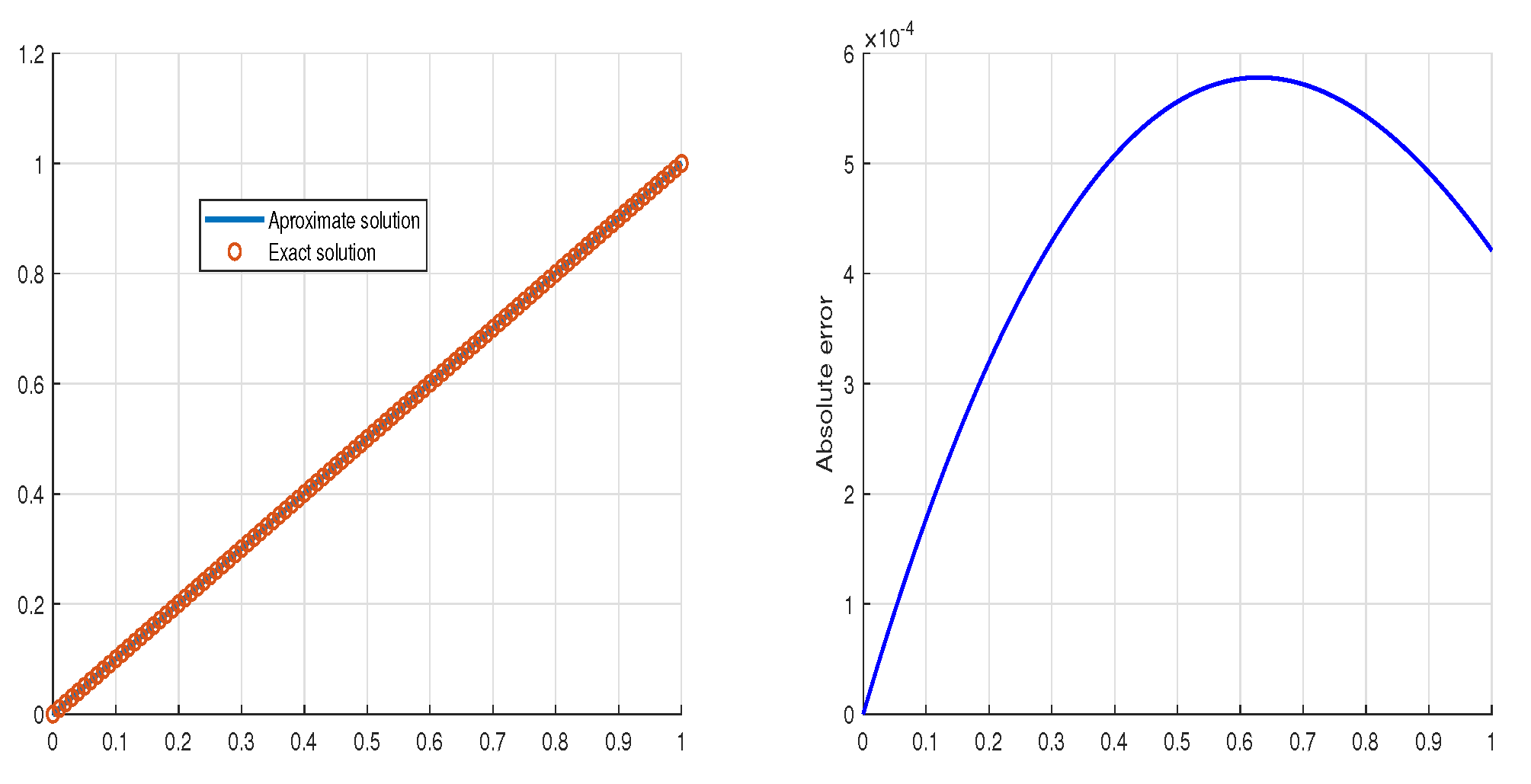
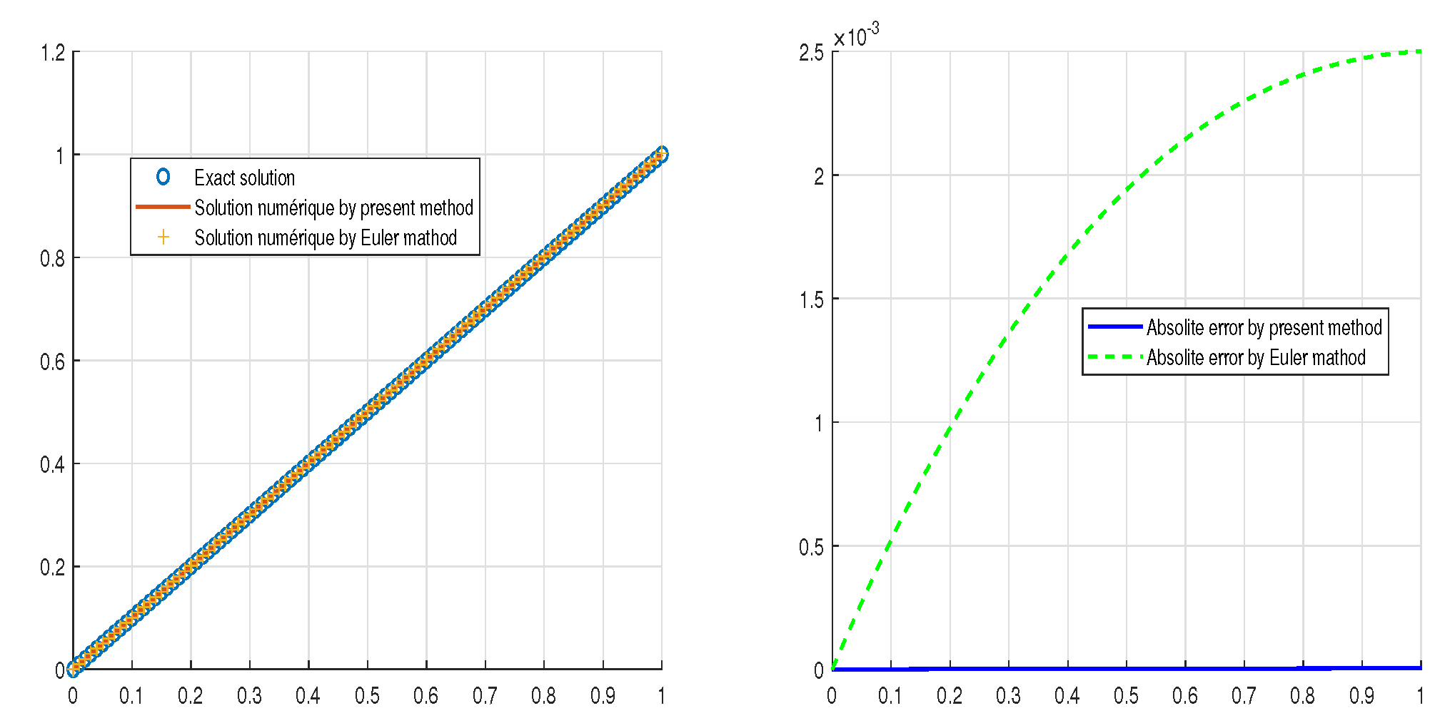
In this section, we present the numerical approximation of the MLCF fractional derivative. Consider a function $u(\lambda )\in H^1(a,b)$ and define the interval $J=[0,T]$. Let h be a constant step size given by $h=T/n$ for some $n\in \mathbb{N}$, and set ${\lambda }_k=kh$. Our goal is to derive a numerical approximation for the integral appearing in Equation (3). A straightforward approach is to apply the standard two-point finite forward difference method to approximate the first derivative over the interval J. Evaluating at $\lambda ={\lambda }_n$ for $0<\nu <1$, we obtain the following expression:

$$\begin{array}{cc}\hfill {}^{MLCF}\mathcal{D}_{\lambda }^{\nu ,\alpha }\left[u(\lambda )\right]{|}_{\lambda ={\lambda }_n}& ={\displaystyle \frac{M(\nu ){\mathbb{E}}_{\alpha }{(\frac{\nu }{1-\nu }{\lambda }_n^{\alpha })}^{-1}}{1-\nu }}{\int }_0^{{\lambda }_n}{u}^{\prime }(\tau ){\mathbb{E}}_{\alpha }\left(\nu {\displaystyle \frac{{\tau }^{\alpha }}{1-\nu }}\right)d\tau \hfill \\ & \approx {\displaystyle \frac{M(\nu ){\mathbb{E}}_{\alpha }{(\frac{\nu }{1-\nu }{\lambda }_n^{\alpha })}^{-1}}{1-\nu }}\sum _{k=0}^{n-1}\left[{\displaystyle \frac{u_{k+1}-u_k}{h}}+\mathcal{O}(h)\right]{\int }_{{\lambda }_k}^{{\lambda }_{k+1}}{\mathbb{E}}_{\alpha }\left(\nu {\displaystyle \frac{{\tau }^{\alpha }}{1-\nu }}\right)d\tau ,\hfill \end{array}$$

as the integral is subsequently approximated using the two-point trapezoidal quadrature method

$${\int }_a^{b}g(z)\mathrm{d}z\approx {\displaystyle \frac{b-a}{2}}(g(a)+g(b)),$$

Then,

$$\begin{array}{cc}\hfill {}^{MLCF}\mathcal{D}_{\lambda }^{\nu ,\alpha }\left[u(\lambda )\right]{|}_{\lambda ={\lambda }_n}& \approx {\displaystyle \frac{M(\nu ){\mathbb{E}}_{\alpha }{(\frac{\nu }{1-\nu }{\lambda }_n^{\alpha })}^{-1}}{1-\nu }}\sum _{k=0}^{n-1}[{\displaystyle \frac{u_{k+1}-u_k}{h}}\hfill \\ & +\mathcal{O}(h)]{\displaystyle \frac{h}{2}}\left({\mathbb{E}}_{\alpha }(\nu {\displaystyle \frac{{\lambda }_{k+1}^{\alpha }}{1-\nu }})+{\mathbb{E}}_{\alpha }(\nu {\displaystyle \frac{{\lambda }_k^{\alpha }}{1-\nu }})\right).\hfill \end{array}$$

For $n=1,2$, and 3, we, respectively, obtain

$$\begin{array}{cc}\hfill {}^{MLCF}\mathcal{D}_{\lambda }^{\nu ,\alpha }\left[u(\lambda )\right]{|}_{\lambda ={\lambda }_1}& ={\displaystyle \frac{M(\nu ){\mathbb{E}}_{\alpha }{(\frac{\nu }{1-\nu }{\lambda }_1)}^{-1}}{2(1-\nu )}}(u_1-u_0)\left({\mathbb{E}}_{\alpha }(\nu {\displaystyle \frac{{\lambda }_1^{\alpha }}{1-\nu }})+{\mathbb{E}}_{\alpha }(\nu {\displaystyle \frac{{\lambda }_0^{\alpha }}{1-\nu }})\right)\hfill \\ \hfill {}^{MLCF}\mathcal{D}_{\lambda }^{\nu ,\alpha }\left[u(\lambda )\right]{|}_{\lambda ={\lambda }_2}& ={\displaystyle \frac{M(\nu ){\mathbb{E}}_{\alpha }{(\frac{\nu }{1-\nu }{\lambda }_2)}^{-1}}{2(1-\nu )}}[(u_1-u_0)\left({\mathbb{E}}_{\alpha }(\nu {\displaystyle \frac{{\lambda }_1^{\alpha }}{1-\nu }})+{\mathbb{E}}_{\alpha }(\nu {\displaystyle \frac{{\lambda }_0^{\alpha }}{1-\nu }})\right)\hfill \\ \hfill & +(u_2-u_1)\left({\mathbb{E}}_{\alpha }(\nu {\displaystyle \frac{{\lambda }_2^{\alpha }}{1-\nu }})+{\mathbb{E}}_{\alpha }(\nu {\displaystyle \frac{{\lambda }_1^{\alpha }}{1-\nu }})\right)]\hfill \\ \hfill {}^{MLCF}\mathcal{D}_{\lambda }^{\nu ,\alpha }\left[u(\lambda )\right]{|}_{\lambda ={\lambda }_3}& ={\displaystyle \frac{M(\nu ){\mathbb{E}}_{\alpha }{(\frac{\nu }{1-\nu }{\lambda }_3)}^{-1}}{2(1-\nu )}}[(u_1-u_0)\left({\mathbb{E}}_{\alpha }(\nu {\displaystyle \frac{{\lambda }_1^{\alpha }}{1-\nu }})+{\mathbb{E}}_{\alpha }(\nu {\displaystyle \frac{{\lambda }_0^{\alpha }}{1-\nu }})\right)\hfill \\ \hfill & +(u_2-u_1)({\mathbb{E}}_{\alpha }(\nu {\displaystyle \frac{{\lambda }_2^{\alpha }}{1-\nu }})\hfill \\ \hfill & +{\mathbb{E}}_{\alpha }(\nu {\displaystyle \frac{{\lambda }_1^{\alpha }}{1-\nu }}))+(u_3-u_2)\left({\mathbb{E}}_{\alpha }(\nu {\displaystyle \frac{{\lambda }_3^{\alpha }}{1-\nu }})+{\mathbb{E}}_{\alpha }(\nu {\displaystyle \frac{{\lambda }_2^{\alpha }}{1-\nu }})\right)].\hfill \end{array}$$

(4)

Continuing in the same way, we obtain

$${}^{MLCF}\mathcal{D}_{\lambda }^{\nu ,\alpha }\left[u(\lambda )\right]{|}_{\lambda ={\lambda }_n}={\displaystyle \frac{M(\nu ){\mathbb{E}}_{\alpha }{(\frac{\nu }{1-\nu }{\lambda }_n^{\alpha })}^{-1}}{(1-\nu )2}}\sum _{k=0}^{n-1}(u_{k+1}-u_k)\left({\mathbb{E}}_{\alpha }(\nu {\displaystyle \frac{{\lambda }_{k+1}^{\alpha }}{1-\nu }})+{\mathbb{E}}_{\alpha }(\nu {\displaystyle \frac{{\lambda }_k^{\alpha }}{1-\nu }})\right).$$

One can replace k with $k-1$ to obtain the following form:

$${}^{MLCF}\mathcal{D}_{\lambda }^{\nu ,\alpha }\left[u(\lambda )\right]{|}_{\lambda ={\lambda }_n}={\displaystyle \frac{M(\nu ){\mathbb{E}}_{\alpha }{(\frac{\nu }{1-\nu }{\lambda }_n^{\alpha })}^{-1}}{(1-\nu )2}}\sum _{k=1}^n(u_{n-k+1}-u_{n-k})\left({\mathbb{E}}_{\alpha }(\nu {\displaystyle \frac{{\lambda }_{n-k+1}^{\alpha }}{1-\nu }})+{\mathbb{E}}_{\alpha }(\nu {\displaystyle \frac{{\lambda }_{n-k}^{\alpha }}{1-\nu }})\right).$$

(5)

Equation (5) represents a first-order time discretization of the MLCF derivative. Based on this, the following theorem is formulated.

Theorem 1.

Consider dividing the interval $[0,T]$ into n equal subintervals, each of width $h=T/n$, using the nodes ${\lambda }_k=kh$ for $k=0,1,\dots ,n$. This leads to the following expression:

$$\begin{array}{cc}\hfill {}^{MLCF}\mathcal{D}_{\lambda }^{\nu ,\alpha }(u,h,\nu )& ={\displaystyle \frac{M(\nu ){\mathbb{E}}_{\alpha }{(\frac{\nu }{1-\nu }{\lambda }_n^{\alpha })}^{-1}}{2(1-\nu )}}\sum _{k=1}^n(u_{n-k+1}-u_{n-k})\left({\mathbb{E}}_{\alpha }(\nu {\displaystyle \frac{{\lambda }_{n-k+1}^{\alpha }}{1-\nu }})+{\mathbb{E}}_{\alpha }(\nu {\displaystyle \frac{{\lambda }_{n-k}^{\alpha }}{1-\nu }})\right)\hfill \\ \hfill & +{\displaystyle \frac{M(\nu ){\mathbb{E}}_{\alpha }{(\frac{\nu }{1-\nu }{\lambda }_n^{\alpha })}^{-1}}{2(1-\nu )}}\sum _{k=1}^n\left({\mathbb{E}}_{\alpha }(\nu {\displaystyle \frac{{\lambda }_{n-k+1}^{\alpha }}{1-\nu }})+{\mathbb{E}}_{\alpha }(\nu {\displaystyle \frac{{\lambda }_{n-k}^{\alpha }}{1-\nu }})\right)\mathcal{O}(h^2),\hfill \end{array}$$

(6)

which is the proposed numerical approximation to the MLCF derivative. In addition, we have

$${}^{MLCF}\mathcal{D}_{\lambda }^{\nu ,\alpha }\left[u(\lambda )\right]{|}_{\lambda ={\lambda }_n}={}^{MLCF}\mathcal{D}_{\lambda }^{\nu ,\alpha }(u,h,\nu )-E_{MLCF}(u,h,\nu ),{\lambda }_n>0,0<\nu <1.$$

Additionally, if $u(\lambda )\in C^1[0,T]$, there exists a constant $A_{\nu }$ that depends solely on ν, such that the error term $E_{MLCF}(u,h,\nu )$ can be expressed in the following manner:

$$\left|E_{MLCF}(u,h,\nu )\right|\le A_{\nu }{∥u^{\prime }∥}_{\infty }{T}^{\nu }h=\mathcal{O}(h).$$

Proof. 

Based on the previous steps in Section 4, we obtain the following:

$$\begin{array}{cc}\hfill {}^{MLCF}\mathcal{D}_{\lambda }^{\nu ,\alpha }(u,h,\nu )& ={\displaystyle \frac{M(\nu ){\mathbb{E}}_{\alpha }{(\frac{\nu }{1-\nu }{\lambda }_n^{\alpha })}^{-1}}{2(1-\nu )}}\sum _{k=1}^n(u_{n-k+1}-u_{n-k})\left({\mathbb{E}}_{\alpha }(\nu {\displaystyle \frac{{\lambda }_{n-k+1}^{\alpha }}{1-\nu }})+{\mathbb{E}}_{\alpha }(\nu {\displaystyle \frac{{\lambda }_{n-k}^{\alpha }}{1-\nu }})\right)\hfill \\ \hfill & +{\displaystyle \frac{M(\nu ){\mathbb{E}}_{\alpha }{(\frac{\nu }{1-\nu }{\lambda }_n^{\alpha })}^{-1}}{2(1-\nu )}}\sum _{k=1}^n\left({\mathbb{E}}_{\alpha }(\nu {\displaystyle \frac{{\lambda }_{n-k+1}^{\alpha }}{1-\nu }})+{\mathbb{E}}_{\alpha }(\nu {\displaystyle \frac{{\lambda }_{n-k}^{\alpha }}{1-\nu }})\right)\mathcal{O}(h^2),\hfill \end{array}$$

(7)

By considering the third term in Equation (7), we obtain

$${\displaystyle \frac{M(\nu ){\mathbb{E}}_{\alpha }{(\frac{\nu }{1-\nu }{\lambda }_n^{\alpha })}^{-1}}{2(1-\nu )}}\sum _{k=1}^n\left({\mathbb{E}}_{\alpha }(\nu {\displaystyle \frac{{\lambda }_{n-k+1}^{\alpha }}{1-\nu }})+{\mathbb{E}}_{\alpha }(\nu {\displaystyle \frac{{\lambda }_{n-k}^{\alpha }}{1-\nu }})\right)\mathcal{O}(h^2).$$

   □

The next section presents several test cases selected to evaluate the effectiveness of the aforementioned approximations.

5. Examples

To evaluate the effectiveness of the proposed numerical approximation (5), two distinct mathematical functions were selected for testing and two applications. The computations were conducted for fractional orders $\alpha \in \{0.5,0.7,0.8,0.9,1\}$ and $\nu \in \{0.5,0.7,0.8,0.9\}$, assuming $M(\nu )=1$. The test cases and their corresponding numerical simulations are summarized in

Table 1. The absolute errors for different $\alpha$ and v.

	$\alpha =0.5$		$\alpha =0.7$
$\nu$	$h={10}^{-2}$	$h={10}^{-3}$	$h={10}^{-2}$	$h={10}^{-3}$
$0.5$	$7.8521\times {10}^{-5}$	$2.8099\times {10}^{-6}$	$1.7050\times {10}^{-5}$	$5.1342\times {10}^{-7}$
$0.7$	$1.4702\times {10}^{-4}$	$1.3851\times {10}^{-6}$	$8.1065\times {10}^{-5}$	$6.9029\times {10}^{-7}$
$0.8$	$6.6638\times {10}^{-4}$	$6.6666\times {10}^{-6}$	$3.0124\times {10}^{-4}$	$3.0064\times {10}^{-6}$
$0.9$	$6.6773\times {10}^{-3}$	$6.7493\times {10}^{-5}$	$1.9215\times {10}^{-3}$	$1.9232\times {10}^{-5}$
	$\alpha =0.8$		$\alpha =1$
$\nu$	$h={10}^{-2}$	$h={10}^{-3}$	$h={10}^{-2}$	$h={10}^{-3}$
$0.5$	$2.6185\times {10}^{-6}$	$1.4263\times {10}^{-7}$	$1.0535\times {10}^{-5}$	$1.0535\times {10}^{-7}$
$0.7$	$6.8827\times {10}^{-5}$	$6.2163\times {10}^{-7}$	$5.8529\times {10}^{-5}$	$5.8530\times {10}^{-7}$
$0.8$	$2.3386\times {10}^{-4}$	$2.3281\times {10}^{-6}$	$1.6361\times {10}^{-4}$	$1.6361\times {10}^{-6}$
$0.9$	$1.2985\times {10}^{-3}$	$1.2990\times {10}^{-5}$	$7.4981\times {10}^{-4}$	$7.4991\times {10}^{-6}$

and

Table 2. The absolute errors for different $\nu$ and h.

$\mathit{\nu }$	$\mathit{h}={10}^{-2}$	$\mathit{h}={10}^{-3}$
$0.5$	$1.4024\times {10}^{-5}$	$1.4025\times {10}^{-7}$
$0.7$	$5.9311\times {10}^{-5}$	$5.9311\times {10}^{-7}$
$0.8$	$1.4276\times {10}^{-4}$	$1.4276\times {10}^{-6}$
$0.9$	$5.3376\times {10}^{-4}$	$5.3379\times {10}^{-6}$

. MATLAB R2020b was used to perform the numerical computations.

Example 1.

Let function $u(\lambda ):=\lambda ,\lambda \in [0,1]$. The ${}^{MLCF}\mathcal{D}_{\lambda }^{\nu ,\alpha }$ of λ is

$$\begin{array}{cc}\hfill {}^{MLCF}\mathcal{D}_{\lambda }^{\nu ,\alpha }u(\lambda )& ={\displaystyle \frac{M(\nu ){\mathbb{E}}_{\alpha }{(\frac{\nu }{1-\nu }{\lambda }^{\alpha })}^{-1}}{1-\nu }}{\int }_0^{\lambda }{\mathbb{E}}_{\alpha }({\displaystyle \frac{\nu }{1-\nu }}{s}^{\alpha })ds\hfill \\ & ={\displaystyle \frac{M(\nu ){\mathbb{E}}_{\alpha }{(\frac{\nu }{1-\nu }{\lambda }^{\alpha })}^{-1}}{1-\nu }}{\int }_0^{\lambda }{\mathbb{E}}_{\alpha }({\displaystyle \frac{\nu }{1-\nu }}{s}^{\alpha })ds,\hfill \end{array}$$

since

$${\int }_0^z{\mathbb{E}}_{\alpha ,\beta }(c{\lambda }^{\alpha }){\lambda }^{\beta -1}d\lambda =z^{\beta }{\mathbb{E}}_{\alpha ,\beta +1}(c{z}^{\alpha }),$$

so

$$\begin{array}{cc}\hfill {}^{MLCF}\mathcal{D}_{\lambda }^{\nu ,\alpha }u(\lambda )& ={\displaystyle \frac{M(\nu ){\mathbb{E}}_{\alpha }{(\frac{\nu }{1-\nu }{\lambda }^{\alpha })}^{-1}}{1-\nu }}\lambda {\mathbb{E}}_{\alpha ,2}({\displaystyle \frac{\nu }{1-\nu }}{\lambda }^{\alpha }).\hfill \end{array}$$

In Figure 1, Figure 2, Figure 3, Figure 4, Figure 5, Figure 6, Figure 7, Figure 8, Figure 9, Figure 10, Figure 11, Figure 12, Figure 13, Figure 14, Figure 15 and Figure 16, we plot the MLCF of function u, the numerical approximation of the MLCF of u, and absolute errors for deferential v and $\alpha$.

Example 2.

Let $u(\lambda )=sin(\lambda )$. Then, we have

$${}^{MLCF}\mathcal{D}_{\lambda }^{\nu ,\alpha }\left[u(\lambda )\right]={\displaystyle \frac{-\nu e^{\frac{\nu }{\nu -1}\lambda }+\nu cos(\lambda )+(1-\nu )sin(\lambda )}{1-2\nu +2{\nu }^2}}.$$

In Figure 17, Figure 18, Figure 19 and Figure 20, we plot the MLCF of function u, the numerical approximation of the MLCF of u, and absolute errors for deferential v and $\alpha$.

Application 1

Consider the following fractional problem:

$$\begin{array}{cc}\hfill {}^{MLCF}\mathcal{D}_{\lambda }^{\nu ,\alpha }u(\lambda )& =\lambda f(\lambda ),\lambda \in ]0,1],\hfill \\ \hfill u(0)& =0,\hfill \end{array}$$

(8)

where

$$f(\lambda )={\displaystyle \frac{M(\nu ){\mathbb{E}}_{\alpha }{(\frac{\nu }{1-\nu }{\lambda }^{\alpha })}^{-1}}{1-\nu }}{\mathbb{E}}_{\alpha ,2}({\displaystyle \frac{\nu }{1-\nu }}{\lambda }^{\alpha }).$$

The exact solution is $u(\lambda )=\lambda$. Consider dividing the interval $[0,1]$ into n equal subintervals, each of width $h=1/n$, using the nodes ${\lambda }_k=kh$ for $k=0,1,\dots ,n$. from Equation (8), we have

$$\begin{array}{c}\hfill {\displaystyle \frac{M(\nu ){\mathbb{E}}_{\alpha }{(\frac{\nu }{1-\nu }{\lambda }_k^{\alpha })}^{-1}}{2(1-\nu )}}\sum _{i=1}^k(u_{k-i+1}-u_{k-i})\left({\mathbb{E}}_{\alpha }(\nu {\displaystyle \frac{{\lambda }_{k-i+1}^{\alpha }}{1-\nu }})+{\mathbb{E}}_{\alpha }(\nu {\displaystyle \frac{{\lambda }_{k-i}^{\alpha }}{1-\nu }})\right)={\lambda }_{k}f({\lambda }_k),\end{array}$$

for $k=1,\dots ,n$. Then,

$$\begin{array}{cc}& {\displaystyle \frac{M(\nu ){\mathbb{E}}_{\alpha }{(\frac{\nu }{1-\nu }{\lambda }_k^{\alpha })}^{-1}}{2(1-\nu )}}{u}_k\left({\mathbb{E}}_{\alpha }(\nu {\displaystyle \frac{{\lambda }_k^{\alpha }}{1-\nu }})+{\mathbb{E}}_{\alpha }(\nu {\displaystyle \frac{{\lambda }_{k-1}^{\alpha }}{1-\nu }})\right)={\lambda }_{k}f({\lambda }_k)\hfill \\ & +{\displaystyle \frac{M(\nu ){\mathbb{E}}_{\alpha }{(\frac{\nu }{1-\nu }{\lambda }_k^{\alpha })}^{-1}}{2(1-\nu )}}{u}_{k-1}\left({\mathbb{E}}_{\alpha }(\nu {\displaystyle \frac{{\lambda }_k^{\alpha }}{1-\nu }})+{\mathbb{E}}_{\alpha }(\nu {\displaystyle \frac{{\lambda }_{k-1}^{\alpha }}{1-\nu }})\right)\hfill \\ & -{\displaystyle \frac{M(\nu ){\mathbb{E}}_{\alpha }{(\frac{\nu }{1-\nu }{\lambda }_k^{\alpha })}^{-1}}{2(1-\nu )}}\sum _{i=2}^k(u_{k-i+1}-u_{k-i})\left({\mathbb{E}}_{\alpha }(\nu {\displaystyle \frac{{\lambda }_{k-i+1}^{\alpha }}{1-\nu }})+{\mathbb{E}}_{\alpha }(\nu {\displaystyle \frac{{\lambda }_{k-i}^{\alpha }}{1-\nu }})\right).\hfill \end{array}$$

Let

$$\left\{\begin{array}{cc}{a}_k={\displaystyle \frac{M(\nu ){\mathbb{E}}_{\alpha }{(\frac{\nu }{1-\nu }{\lambda }_k^{\alpha })}^{-1}}{2(1-\nu )}}\left({\mathbb{E}}_{\alpha }(\nu {\displaystyle \frac{{\lambda }_k^{\alpha }}{1-\nu }})+{\mathbb{E}}_{\alpha }(\nu {\displaystyle \frac{{\lambda }_{k-1}^{\alpha }}{1-\nu }})\right),\hfill & k=1,\dots ,n,\hfill \\ b_k={\displaystyle \frac{M(\nu ){\mathbb{E}}_{\alpha }{(\frac{\nu }{1-\nu }{\lambda }_k^{\alpha })}^{-1}}{2(1-\nu )}},\hfill & k=1,\dots ,n,\hfill \\ c_{k,i}=\left({\mathbb{E}}_{\alpha }(\nu {\displaystyle \frac{{\lambda }_{k-i+1}^{\alpha }}{1-\nu }})+{\mathbb{E}}_{\alpha }(\nu {\displaystyle \frac{{\lambda }_{k-i}^{\alpha }}{1-\nu }})\right),\hfill & k=2,\dots ,n,i=2,\dots ,k.\hfill \end{array}\right.$$

Therefore,

$$\left\{\begin{array}{cc}{u}_1={\displaystyle \frac{{\lambda }_{1}f({\lambda }_1)}{a_1}}+u_0,\hfill & \\ u_k={\displaystyle \frac{{\lambda }_{k}f({\lambda }_k)}{a_k}}+u_{k-1}-{\displaystyle \frac{b_k}{a_k}}\sum _{i=2}^k(u_{k-i+1}-u_{k-i})c_{k,i},\hfill & k=2,\dots ,n.\hfill \end{array}\right.$$

In Algorithm 1, we present the numerical method for solving Equation (8).

Algorithm 1 Numerical method for solving Equation (8).

Input: $n\in \mathbb{N}$, $\alpha ,\nu \in [0,1]$.   Set $h={\displaystyle \frac{1}{n}}$.   Set ${\lambda }_k=kh$ for $k=0,1,\dots ,n$.   Compute $a_k={\displaystyle \frac{M(\nu ){\mathbb{E}}_{\alpha }{(\frac{\nu }{1-\nu }{\lambda }_k^{\alpha })}^{-1}}{2(1-\nu )}}\left({\mathbb{E}}_{\alpha }(\nu {\displaystyle \frac{{\lambda }_k^{\alpha }}{1-\nu }})+{\mathbb{E}}_{\alpha }(\nu {\displaystyle \frac{{\lambda }_{k-1}^{\alpha }}{1-\nu }})\right),k=1,\dots ,n$.   Compute $b_k={\displaystyle \frac{M(\nu ){\mathbb{E}}_{\alpha }{(\frac{\nu }{1-\nu }{\lambda }_k^{\alpha })}^{-1}}{2(1-\nu )}},k=1,\dots ,n.$   Compute $c_{k,i}=\left({\mathbb{E}}_{\alpha }(\nu {\displaystyle \frac{{\lambda }_{k-i+1}^{\alpha }}{1-\nu }})+{\mathbb{E}}_{\alpha }(\nu {\displaystyle \frac{{\lambda }_{k-i}^{\alpha }}{1-\nu }})\right),k=2,\dots ,n,i=2,\dots ,k.$   Compute $u_1={\displaystyle \frac{{\lambda }_{1}f({\lambda }_1)}{a_1}}+u_0.$   Compute $u_k={\displaystyle \frac{{\lambda }_{k}f({\lambda }_k)}{a_k}}+u_{k-1}-{\displaystyle \frac{b_k}{a_k}}{\sum }_{i=2}^k(u_{k-i+1}-u_{k-i})c_{k,i},k=2,\dots ,n.$

Output: The approximate solution $u_k$.

In Figure 21 and Figure 22, we plot the exact solution, numerical solution, and absolute error for different $\nu$ and $\alpha$.

Application 2

Consider the following fractional problem:

$$\begin{array}{cc}\hfill {}^{MLCF}\mathcal{D}_{\lambda }^{\nu ,\alpha }u(\lambda )& =u(\lambda )\left(f(\lambda )+1\right)-{\lambda }^{\alpha },\lambda \in ]0,1],\hfill \\ \hfill u(0)& =0,\hfill \end{array}$$

(9)

where

$$f(\lambda )={\displaystyle \frac{M(\nu )\alpha }{1-\nu }}{\mathbb{E}}_{\alpha }{({\displaystyle \frac{\nu }{1-\nu }}{\lambda }^{\alpha })}^{-1}{\mathbb{E}}_{\alpha ,\alpha +1}({\displaystyle \frac{\nu }{1-\nu }}{\lambda }^{\alpha }).$$

The exact solution is $u(\lambda )={\lambda }^{\alpha }$. Consider dividing the interval $[0,1]$ into n equal subintervals, each of width $h=1/n$, using the nodes ${\lambda }_k=kh$ for $k=0,1,\dots ,n$. From Equation (9), we have

$$\begin{array}{c}\hfill {\displaystyle \frac{M(\nu ){\mathbb{E}}_{\alpha }{(\frac{\nu }{1-\nu }{\lambda }_k^{\alpha })}^{-1}}{2(1-\nu )}}\sum _{i=1}^k(u_{k-i+1}-u_{k-i})\left({\mathbb{E}}_{\alpha }(\nu {\displaystyle \frac{{\lambda }_{k-i+1}^{\alpha }}{1-\nu }})+{\mathbb{E}}_{\alpha }(\nu {\displaystyle \frac{{\lambda }_{k-i}^{\alpha }}{1-\nu }})\right)=u_k\left(f({\lambda }_k)+1\right)-{\lambda }_k^{\alpha },\end{array}$$

for $k=1,\dots ,n$. Then,

$$\begin{array}{cc}& {\displaystyle \frac{M(\nu ){\mathbb{E}}_{\alpha }{(\frac{\nu }{1-\nu }{\lambda }_k^{\alpha })}^{-1}}{2(1-\nu )}}{u}_k\left({\mathbb{E}}_{\alpha }(\nu {\displaystyle \frac{{\lambda }_k^{\alpha }}{1-\nu }})+{\mathbb{E}}_{\alpha }(\nu {\displaystyle \frac{{\lambda }_{k-1}^{\alpha }}{1-\nu }})\right)=u_k\left(f({\lambda }_k)+1\right)-{\lambda }_k^{\alpha }\hfill \\ & +{\displaystyle \frac{M(\nu ){\mathbb{E}}_{\alpha }{(\frac{\nu }{1-\nu }{\lambda }_k^{\alpha })}^{-1}}{2(1-\nu )}}{u}_{k-1}\left({\mathbb{E}}_{\alpha }(\nu {\displaystyle \frac{{\lambda }_k^{\alpha }}{1-\nu }})+{\mathbb{E}}_{\alpha }(\nu {\displaystyle \frac{{\lambda }_{k-1}^{\alpha }}{1-\nu }})\right)\hfill \\ & -{\displaystyle \frac{M(\nu ){\mathbb{E}}_{\alpha }{(\frac{\nu }{1-\nu }{\lambda }_k^{\alpha })}^{-1}}{2(1-\nu )}}\sum _{i=2}^k(u_{k-i+1}-u_{k-i})\left({\mathbb{E}}_{\alpha }(\nu {\displaystyle \frac{{\lambda }_{k-i+1}^{\alpha }}{1-\nu }})+{\mathbb{E}}_{\alpha }(\nu {\displaystyle \frac{{\lambda }_{k-i}^{\alpha }}{1-\nu }})\right).\hfill \end{array}$$

Let

$$\left\{\begin{array}{cc}{a}_k={\displaystyle \frac{M(\nu ){\mathbb{E}}_{\alpha }{(\frac{\nu }{1-\nu }{\lambda }_k^{\alpha })}^{-1}}{2(1-\nu )}}\left({\mathbb{E}}_{\alpha }(\nu {\displaystyle \frac{{\lambda }_k^{\alpha }}{1-\nu }})+{\mathbb{E}}_{\alpha }(\nu {\displaystyle \frac{{\lambda }_{k-1}^{\alpha }}{1-\nu }})\right)-\left(f({\lambda }_k)+1\right),\hfill & k=1,\dots ,n,\hfill \\ b_k={\displaystyle \frac{M(\nu ){\mathbb{E}}_{\alpha }{(\frac{\nu }{1-\nu }{\lambda }_k^{\alpha })}^{-1}}{2(1-\nu )}}\left({\mathbb{E}}_{\alpha }(\nu {\displaystyle \frac{{\lambda }_k^{\alpha }}{1-\nu }})+{\mathbb{E}}_{\alpha }(\nu {\displaystyle \frac{{\lambda }_{k-1}^{\alpha }}{1-\nu }})\right),\hfill & k=1,\dots ,n,\hfill \\ d_k={\displaystyle \frac{M(\nu ){\mathbb{E}}_{\alpha }{(\frac{\nu }{1-\nu }{\lambda }_k^{\alpha })}^{-1}}{2(1-\nu )}},\hfill & k=1,\dots ,n,\hfill \\ c_{k,i}=\left({\mathbb{E}}_{\alpha }(\nu {\displaystyle \frac{{\lambda }_{k-i+1}^{\alpha }}{1-\nu }})+{\mathbb{E}}_{\alpha }(\nu {\displaystyle \frac{{\lambda }_{k-i}^{\alpha }}{1-\nu }})\right),\hfill & k=2,\dots ,n,i=2,\dots ,k.\hfill \end{array}\right.$$

Therefore,

$$\left\{\begin{array}{cc}{u}_1=-{\displaystyle \frac{{\lambda }_1^{\alpha }}{a_1}}+{\displaystyle \frac{b_1}{a_1}}{u}_0,\hfill & \\ u_k=-{\displaystyle \frac{{\lambda }_k^{\alpha }}{a_k}}+{\displaystyle \frac{b_k}{a_k}}{u}_{k-1}-{\displaystyle \frac{d_k}{a_k}}\sum _{i=2}^k(u_{k-i+1}-u_{k-i})c_{k,i},\hfill & k=2,\dots ,n.\hfill \end{array}\right.$$

In Algorithm 2, we present the numerical method for solving Equation (9).

Algorithm 2 Numerical method for solving Equation (9).

Input: $n\in \mathbb{N}$, $\alpha ,\nu \in [0,1]$.   Set $h={\displaystyle \frac{1}{n}}$.   Set ${\lambda }_k=kh$ for $k=0,1,\dots ,n$.   Compute $a_k={\displaystyle \frac{M(\nu ){\mathbb{E}}_{\alpha }{(\frac{\nu }{1-\nu }{\lambda }_k^{\alpha })}^{-1}}{2(1-\nu )}}\left({\mathbb{E}}_{\alpha }(\nu {\displaystyle \frac{{\lambda }_k^{\alpha }}{1-\nu }})+{\mathbb{E}}_{\alpha }(\nu {\displaystyle \frac{{\lambda }_{k-1}^{\alpha }}{1-\nu }})\right)-\left(f({\lambda }_k)+1\right),k=1,\dots ,n$.   Compute $b_k={\displaystyle \frac{M(\nu ){\mathbb{E}}_{\alpha }{(\frac{\nu }{1-\nu }{\lambda }_k^{\alpha })}^{-1}}{2(1-\nu )}}\left({\mathbb{E}}_{\alpha }(\nu {\displaystyle \frac{{\lambda }_k^{\alpha }}{1-\nu }})+{\mathbb{E}}_{\alpha }(\nu {\displaystyle \frac{{\lambda }_{k-1}^{\alpha }}{1-\nu }})\right),k=1,\dots ,n.$   Compute $d_k={\displaystyle \frac{M(\nu ){\mathbb{E}}_{\alpha }{(\frac{\nu }{1-\nu }{\lambda }_k^{\alpha })}^{-1}}{2(1-\nu )}},k=1,\dots ,n.$   Compute $c_{k,i}=\left({\mathbb{E}}_{\alpha }(\nu {\displaystyle \frac{{\lambda }_{k-i+1}^{\alpha }}{1-\nu }})+{\mathbb{E}}_{\alpha }(\nu {\displaystyle \frac{{\lambda }_{k-i}^{\alpha }}{1-\nu }})\right),k=2,\dots ,n,i=2,\dots ,k.$   Compute $u_1=-{\displaystyle \frac{{\lambda }_1^{\alpha }}{a_1}}+{\displaystyle \frac{b_1}{a_1}}{u}_0.$   Compute $u_k=-{\displaystyle \frac{{\lambda }_k^{\alpha }}{a_k}}+{\displaystyle \frac{b_k}{a_k}}{u}_{k-1}-{\displaystyle \frac{d_k}{a_k}}{\sum }_{i=2}^k(u_{k-i+1}-u_{k-i})c_{k,i},k=2,\dots ,n.$

Output: The approximate solution $u_k$.

In Figure 23, we plot the exact solution, numerical solution, and the absolute error. In Figure 24, we plot the solution obtained using the MLCF derivative and the solution obtained using the Caputo derivative. In Figure 25, we plot the solution obtained using the MLCF derivative and the solution obtained using the fractional Euler method in [47].

6. Conclusions

This study introduces a new definition for the fractional derivative with a numerical approximation. The error analysis demonstrates that the proposed method converges at the first order, as evidenced by the local truncation error term of the form $\mathcal{O}(h)$. This analysis was extended to a continuous temporal mesh to achieve improved accuracy. Test cases 1 and 2 validate the first-order convergence of the numerical approximation, showing a consistent reduction in the computed absolute errors by one order with each corresponding to a decrease in time step h. In the future, we will study other schemes.

References

1. Sadek, L.; Jarad, F. The general Caputo–Katugampola fractional derivative and numerical approach for solving the fractional differential equations. Alex. Eng. J. 2025, 121, 539–557. [Google Scholar] [CrossRef]
2. Al-Refai, M. On weighted Atangana–Baleanu fractional operators. Adv. Differ. Equ. 2020, 2020, 3. [Google Scholar] [CrossRef]
3. Sadek, L.; Baleanu, D.; Abdo, M.S.; Shatanawi, W. Introducing novel Θ-fractional operators: Advances in fractional calculus. J. King Saud Univ. Sci. 2024, 36, 103352. [Google Scholar] [CrossRef]
4. Jarad, F.; Abdeljawad, T.; Rashid, S.; Hammouch, Z. More properties of the proportional fractional integrals and derivatives of a function with respect to another function. Adv. Differ. Equ. 2020, 2020, 303. [Google Scholar] [CrossRef]
5. Jarad, F.; Abdeljawad, T.; Shah, K. On the weighted fractional operators of a function with respect to another function. Fractals 2020, 28, 2040011. [Google Scholar] [CrossRef]
6. Sousa, J.V.D.C.; De Oliveira, E.C. Leibniz type rule: ψ-Hilfer fractional operator. Commun. Nonlinear Sci. Numer. Simul. 2019, 77, 305–311. [Google Scholar] [CrossRef]
7. Sadek, L. Controllability, observability, and stability of ϕ-conformable fractional linear dynamical systems. Asian J. Control 2024, 26, 2476–2494. [Google Scholar] [CrossRef]
8. Ardjouni, A.; Boulares, H.; Djoudi, A. Stability of nonlinear neutral nabla fractional difference equations. Commun. Optim. Theory 2018, 2018, 8. [Google Scholar]
9. Atangana, A.; Akgül, A.; Owolabi, K.M. Analysis of fractal fractional differential equations. Alex. Eng. J. 2020, 59, 1117–1134. [Google Scholar] [CrossRef]
10. Mathivanan, T.; Bheeman, R.; Prasantha Bharathi Dhandapani, P.B.; Alraddadi, I.; Ahmad, H.; Radwan, T. Monkeypox: A New Mathematical Model Using the Caputo-Fabrizio Fractional Derivative. Fractals 2025, 2025, 2540128. [Google Scholar] [CrossRef]
11. Khan, M.A.; Hammouch, Z.; Baleanu, D. Modeling the dynamics of hepatitis E via the Caputo–Fabrizio derivative. Math. Model. Nat. Phenom. 2019, 14, 311. [Google Scholar] [CrossRef]
12. Hammouch, Z.; Jamil, M.O.; Unlu, C. Dynamics investigation and numerical simulation of fractional-order predator-prey model with Holling type II functional response. Discret. Contin. Dyn. Syst. S 2025, 18, 1230–1266. [Google Scholar] [CrossRef]
13. Baitiche, Z.; Guerbati, K.; Benchohra, M.; Zhou, Y. Boundary value problems for hybrid Caputo fractional differential equations. Mathematics 2019, 7, 282. [Google Scholar] [CrossRef]
14. Abro, K.A.; Memon, A.A.; Memon, A.A. Functionality of circuit via modern fractional differentiations. Analog. Integr. Circuits Signal Process. 2019, 99, 11–21. [Google Scholar] [CrossRef]
15. Arqub, O.A.; Al-Smadi, M. Atangana–Baleanu fractional approach to the solutions of Bagley–Torvik and Painlevé equations in Hilbert space. Chaos Solitons Fractals 2018, 117, 161–167. [Google Scholar] [CrossRef]
16. Qureshi, S.; Yusuf, A. Modeling chickenpox disease with fractional derivatives: From caputo to atangana-baleanu. Chaos Solitons Fractals 2019, 122, 111–118. [Google Scholar] [CrossRef]
17. Sadek, L. Two Numerical Approaches for Solving Fractional Model of Chemical Kinetics Problem via Chebyshev Polynomials. Prog. Fract. Differ. Appl. 2024, 10, 601–613. [Google Scholar]
18. Mahmud, A.A.; Tanriverdi, T.; Muhamad, K.A. Exact traveling wave solutions for (2+1)-dimensional Konopelchenko-Dubrovsky equation by using the hyperbolic trigonometric functions methods. Int. J. Math. Comput. Eng. 2023, 1, 11–24. [Google Scholar] [CrossRef]
19. Jan, A.; Shah, R.A.; Bilal, H.; Almohsen, B.; Jan, R.; Sharma, B.K. Dynamics and stability analysis of enzymatic cooperative chemical reactions in biological systems with time-delayed effects. Partial Differ. Equ. Appl. Math. 2024, 11, 100850. [Google Scholar] [CrossRef]
20. Saad, K.M.; Srivastava, R. Non-standard finite difference and vieta-lucas orthogonal polynomials for the multi-space fractional-order coupled korteweg-de vries equation. Symmetry 2024, 16, 242. [Google Scholar] [CrossRef]
21. Alqhtani, M.; Khader, M.M.; Saad, K.M. Numerical simulation for a high-dimensional chaotic Lorenz system based on Gegenbauer wavelet polynomials. Mathematics 2023, 11, 472. [Google Scholar] [CrossRef]
22. Manickam, A.; Kavitha, M.; Jaison, A.B.; Singh, A.K. A Fractional-Order Mathematical Model of Banana Xanthomonas Wilt Disease Using Caputo Derivatives. Contemp. Math. 2024, 136–156. [Google Scholar] [CrossRef]
23. Sheikh, N.A.; Ali, F.; Saqib, M.; Khan, I.; Jan, S.A.A.; Alshomrani, A.S.; Alghamdi, M.S. Comparison and analysis of the Atangana–Baleanu and Caputo–Fabrizio fractional derivatives for generalized Casson fluid model with heat generation and chemical reaction. Results Phys. 2017, 7, 789–800. [Google Scholar] [CrossRef]
24. Atangana, A.; Baleanu, D. Caputo-Fabrizio derivative applied to groundwater flow within confined aquifer. J. Eng. Mech. 2017, 143, D4016005. [Google Scholar] [CrossRef]
25. Diethelm, K.; Ford, N.J. Analysis of fractional differential equations. J. Math. Anal. Appl. 2002, 265, 229–248. [Google Scholar] [CrossRef]
26. Hilfer, R.; Luchko, Y. Desiderata for fractional derivatives and integrals. Mathematics 2019, 7, 149. [Google Scholar] [CrossRef]
27. Yusuf, A.; Inc, M.; Aliyu, A.I.; Baleanu, D. Efficiency of the new fractional derivative with nonsingular Mittag-Leffler kernel to some nonlinear partial differential equations. Chaos Solitons Fractals 2018, 116, 220–226. [Google Scholar] [CrossRef]
28. Inc, M.; Yusuf, A.; Aliyu, A.I.; Baleanu, D. Investigation of the logarithmic-KdV equation involving Mittag-Leffler type kernel with Atangana–Baleanu derivative. Phys. A Stat. Mech. Its Appl. 2018, 506, 520–531. [Google Scholar] [CrossRef]
29. Caputo, M.; Fabrizio, M. Applications of new time and spatial fractional derivatives with exponential kernels. Prog. Fract. Differ. Appl. 2016, 2, 1–11. [Google Scholar] [CrossRef]
30. Xiao-Jun, X.J.; Srivastava, H.M.; Machado, J.T. A new fractional derivative without singular kernel. Therm. Sci. 2016, 20, 753–756. [Google Scholar]
31. Hallaci, A.; Boulares, H.; Ardjouni, A.; Chaoui, A. On the study of fractional differential equations in a weighted Sobolev space. Bull. Int. Math. Virtual Inst. 2019, 9, 333–343. [Google Scholar]
32. Diethelm, K.; Ford, N.J.; Freed, A.D.; Luchko, Y. Algorithms for the fractional calculus: A selection of numerical methods. Comput. Methods Appl. Mech. Eng. 2005, 194, 743–773. [Google Scholar] [CrossRef]
33. Garrappa, R. Numerical solution of fractional differential equations: A survey and a software tutorial. Mathematics 2018, 6, 16. [Google Scholar] [CrossRef]
34. Qureshi, S.; Rangaig, N.A.; Baleanu, D. New numerical aspects of Caputo-Fabrizio fractional derivative operator. Mathematics 2019, 7, 374. [Google Scholar] [CrossRef]
35. Arshad, S.; Saleem, I.; Akgül, A.; Huang, J.; Tang, Y.; Eldin, S.M. A novel numerical method for solving the Caputo-Fabrizio fractional differential equation. AIMS Math. 2023, 8, 9535–9556. [Google Scholar] [CrossRef]
36. Pariyar, S.; Kafle, J. Caputo-Fabrizio approach to numerical fractional derivatives. BIBECHANA 2023, 20, 126–133. [Google Scholar] [CrossRef]
37. Akman, T.; Yıldız, B.; Baleanu, D. New discretization of Caputo–Fabrizio derivative. Comput. Appl. Math. 2018, 37, 3307–3333. [Google Scholar] [CrossRef]
38. Wei, Y.; Chen, Y.; Cheng, S.; Wang, Y. A note on short memory principle of fractional calculus. Fract. Calc. Appl. Anal. 2017, 20, 1382–1404. [Google Scholar] [CrossRef]
39. Khader, M.M.; Macías-Díaz, J.E.; Román-Loera, A.; Saad, K.M. A Note on a Fractional Extension of the Lotka–Volterra Model Using the Rabotnov Exponential Kernel. Axioms 2024, 13, 71. [Google Scholar] [CrossRef]
40. Caputo, M.; Fabrizio, M. A new definition of fractional derivative without singular kernel. Prog. Fract. Differ. Appl. 2015, 1, 73–85. [Google Scholar]
41. Tunç, O. New Results on the Ulam–Hyers–Mittag–Leffler Stability of Caputo Fractional-Order Delay Differential Equations. Mathematics 2024, 12, 1342. [Google Scholar] [CrossRef]
42. Pal, A. Generalized Integral Transform and Fractional Calculus Operators Involving a Generalized Mittag-Leffler (ML)-Type Function. Comput. Sci. Math. Forum 2023, 7, 42. [Google Scholar]
43. Awais, M.; Kirmani, S.K.N.; Rana, M.; Ahmad, R. Caputo Fabrizio Bézier Curve with Fractional and Shape Parameters. Computers 2024, 13, 206. [Google Scholar] [CrossRef]
44. Almeida, R. Variational Problems Involving a Generalized Fractional Derivative with Dependence on the Mittag–Leffler Function. Fractal Fract. 2023, 7, 477. [Google Scholar] [CrossRef]
45. Chouhan, V.S.; Badsara, A.K.; Shukla, R. Zika Virus Model with the Caputo–Fabrizio Fractional Derivative. Symmetry 2024, 16, 1606. [Google Scholar] [CrossRef]
46. Sadek, L.; Bataineh, A.S.; Talibi Alaoui, H.; Hashim, I. The novel mittag-leffler–galerkin method: Application to a riccati differential equation of fractional order. Fractal Fract. 2023, 7, 302. [Google Scholar] [CrossRef]
47. Jajarmi, A.; Baleanu, D. A new fractional analysis on the interaction of HIV with CD4+ T-cells. Chaos Solitons Fractals 2018, 113, 221–229. [Google Scholar] [CrossRef]
Figure 1. The MLCF of function u, numerical approximation of MLCF of u, and absolute errors with α = ν = 0.5 , h = 0.01 , and h = 0.001 for Example 1.
Symmetry 17 00800 g001
Figure 2. The MLCF of function u, numerical approximation of MLCF of u, and absolute errors with α = 0.5 , ν = 0.7 , h = 0.01 , and h = 0.001 for Example 1.
Symmetry 17 00800 g002
Figure 3. The MLCF of function u, numerical approximation of MLCF of u, and absolute errors with α = 0.5 , ν = 0.8 , h = 0.01 , and h = 0.001 for Example 1.
Symmetry 17 00800 g003
Figure 4. The MLCF of function u, numerical approximation of MLCF of u, and absolute errors with α = 0.5 , ν = 0.9 , h = 0.01 , and h = 0.001 for Example 1.
Symmetry 17 00800 g004
Figure 5. The MLCF of function u, numerical approximation of MLCF of u, and absolute errors with α = 0.7 , ν = 0.5 , h = 0.01 , and h = 0.001 for Example 1.
Symmetry 17 00800 g005
Figure 6. The MLCF of function u, numerical approximation of MLCF of u, and absolute errors with α = 0.7 , ν = 0.7 , h = 0.01 , and h = 0.001 for Example 1.
Symmetry 17 00800 g006
Figure 7. The MLCF of function u, numerical approximation of MLCF of u, and absolute errors with α = 0.7 , ν = 0.8 , h = 0.01 , and h = 0.001 for Example 1.
Symmetry 17 00800 g007
Figure 8. The MLCF of function u, numerical approximation of MLCF of u, and absolute errors with α = 0.7 , ν = 0.9 , h = 0.01 , and h = 0.001 for Example 1.
Symmetry 17 00800 g008
Figure 9. The MLCF of function u, numerical approximation of MLCF of u, and absolute errors with α = 0.8 , ν = 0.5 , h = 0.01 , and h = 0.001 for Example 1.
Symmetry 17 00800 g009
Figure 10. The MLCF of function u, numerical approximation of MLCF of u, and absolute errors with α = 0.8 , ν = 0.7 , h = 0.01 , and h = 0.001 for Example 1.
Symmetry 17 00800 g010
Figure 11. The MLCF of function u, numerical approximation of MLCF of u, and absolute errors with α = 0.8 , ν = 0.8 , h = 0.01 , and h = 0.001 for Example 1.
Symmetry 17 00800 g011
Figure 12. The MLCF of function u, numerical approximation of MLCF of u, and absolute errors with α = 0.8 , ν = 0.9 , h = 0.01 , and h = 0.001 for Example 1.
Symmetry 17 00800 g012
Figure 13. The MLCF of function u, numerical approximation of MLCF of u, and absolute errors with α = 1 , ν = 0.5 , h = 0.01 , and h = 0.001 for Example 1.
Symmetry 17 00800 g013
Figure 14. The MLCF of function u, numerical approximation of MLCF of u, and absolute errors with α = 1 , ν = 0.7 , h = 0.01 , and h = 0.001 for Example 1.
Symmetry 17 00800 g014
Figure 15. The MLCF of function u, numerical approximation of MLCF of u, and absolute errors with α = 1 , ν = 0.8 , h = 0.01 , and h = 0.001 for Example 1.
Symmetry 17 00800 g015
Figure 16. The MLCF of function u, numerical approximation of MLCF of u, and absolute errors with α = 1 , ν = 0.9 , h = 0.01 , and h = 0.001 for Example 1.
Symmetry 17 00800 g016
Figure 17. The MLCF of function u, numerical approximation of MLCF of u, and absolute errors with ν = 0.5 , h = 0.01 , and h = 0.001 for Example 2.
Symmetry 17 00800 g017
Figure 18. The MLCF of function u, numerical approximation of MLCF of u, and absolute errors with ν = 0.7 , h = 0.01 , and h = 0.001 for Example 2.
Symmetry 17 00800 g018
Figure 19. The MLCF of function u, numerical approximation of MLCF of u, and absolute errors with ν = 0.8 , h = 0.01 , and h = 0.001 for Example 2.
Symmetry 17 00800 g019
Figure 20. The MLCF of function u, numerical approximation of MLCF of u, and absolute errors with ν = 0.9 , h = 0.01 , and h = 0.001 for Example 2.
Symmetry 17 00800 g020
Figure 21. The exact solution, numerical solution, and absolute error with α = 0.9 , ν = 0.5 , and h = 0.01 for Application 1.
Symmetry 17 00800 g021
Figure 22. The exact solution, numerical solution, and absolute error with α = 0.8 , ν = 0.4 , and h = 0.01 for Application 1.
Symmetry 17 00800 g022
Figure 23. The exact solution, numerical solution, and absolute error with α = 0.998 , ν = 0.4 , and h = 0.01 for Application 2.
Symmetry 17 00800 g023
Figure 24. The solution using Caputo’s definition with the new definition for Application 2, where α = 0.5 and ν = 0.4 .
Symmetry 17 00800 g024
Figure 25. The exact solution, numerical solution (present method and fractional Euler method in [47]), and absolute errors with α = 1 , ν = 0.4 , and h = 0.01 for Application 2.
Symmetry 17 00800 g025