Abstract
Fractional-order differential equations are prevalent in many scientific fields; hence, their study has seen a renaissance in recent years. The fascinating realm of fractional calculus is explored in this research study, with particular emphasis on the Harry Dym equation. To solve this problem, we use the Laplace Residual Power Series Method (LRPSM) and introduce the New Iterative Method (NIM). Both the mathematical complexity of the Harry Dym problem and the viability of the Caputo operator in this setting are investigated in our work. We go beyond the limitations of traditional mathematical methods to provide novel insights into the results of fractional-order differential equations via careful analysis and cutting-edge procedures. In this paper, we combine theory and practice to provide a novel perspective to the results of high-order fractional differential equations. Our efforts pay off by expanding our knowledge of mathematics and revealing the latent potential of the Harry Dym equation. This study expands researchers’ and mathematicians’ perspectives, bringing in a new and exciting period of progress in the field of fractional calculus.
1. Introduction
The study of the characteristics of integrals and derivatives of orders other than integers is known as fractional calculus (FC). In recent decades, fractional differential equations have been studied to investigate a wide field of scientific topics. FC has attracted greater attention than traditional calculus because of its varied applicability to the study of physical phenomena. Fluid dynamics, signal processing, astronomy, calculus, genetics, kinetics, and a number of other branches of physics have all benefited from the applications of FC to the demonstrations of PDEs [1,2,3,4]. Sadek et al. [5,6,7] introduced -fractional operators, generalizing traditional fractional calculus through adaptive weight functions to define -conformable derivatives -CFD and associated function spaces, supported by foundational theorems. It proposes generalized Bernstein basis functions for solving linear/nonlinear -Caputo fractional differential equations (-FDEs) via collocation methods, extending classical Bernstein polynomials to address applied mathematics problems. Additionally, the work introduces -conformable fractional derivatives/integrals, analyzing the controllability, observability, and stability of -conformable dynamical systems (-CF-DS) through Lyapunov equations and eigenvalue criteria. Theoretical advancements are validated by numerical experiments, demonstrating convergence and efficacy in solving complex fractional models, bridging abstract operator theory with practical computational frameworks for differential equations and dynamical systems.
Nonlinear partial differential equations (PDEs) represent important techniques in many scientific and technological disciplines. Nonlinear PDEs contain terms that depend nonlinearly on the unknown function and its derivatives, making them more difficult to solve than linear PDEs, for which there are recognized techniques. As a result, complex mathematical frameworks are common, which can make it very hard or even impossible to find exact solutions. So, scientists and professionals use different approaches to solve these problems. Numerous studies have delved into these PDEs, employing a diverse range of analytical and numerical techniques. These encompass methodologies like the Homotopy perturbation technique [8], the Exp-function scheme [9], Homotopy analysis technique [10], subequation technique [11], first integral approach [12], rational function strategy [13], auxiliary equation procedure [14], quasi-wavelet process [15], fractional complex transform [16], and fractional Reduced Differential Transform technique [17].
Kruskal and Moser [18] (1974) performed an important investigation that marked the first exploration of the Harry Dym equation (HDEq) in the field. This paper contributes to the investigation of nonlinear HDEq by introducing fractional operators, thus enhancing our comprehension of its complex dynamics:
having the initial condition
This HDEq does not have the Painleve property, but it is applied to pinpoint applications in a number of physical techniques. The HDEq has connections to the Korteweg–de Vries equation, and the implementation of this equation to hydrodynamics issues has been discovered. The HDEq fractional model was examined by Kumar et al. [19], who used HPM to achieve an approximation of the solution. A system of variation and modulation is connected to this equation, making HDEq a fully integrable, nonlinear evolution problem. Given that it adheres to the conversion rules, the HDEq is quite significant. The precise traveling wave solutions to the HDEq were researched by Mokhtari [20]. In order to analyze the precise results in explicit forms of the time FHDEq, Huanga and Zhdanovb [21] applied a Lie symmetry technique. The finite difference approach was utilized by Yokus and Glbahar [22] to get approximations of the findings of HDEq with fractional derivative. For the analytical results of linear and nonlinear systems, he came up with the notion of the homotopy perturbation technique (HPM) [23,24]. Later, several writers [25] investigated the responses of HPM to these difficulties. To solve nonlinear vibration systems, Nadeem and Li [26,27] combined HPM with the Laplace transform.
The Laplace Residual Power Series Method (LRPSM) is an analytical technique for approximating solutions to differential equations. Nonlinear differential equations, which are notoriously difficult to solve, benefit greatly from this method. By expanding the results into a power series in terms of a small parameter, this method provides a systematic approximation. The LRPSM may be useful when perturbation theory is unsuccessful. This method is helpful for scientists and engineers researching advanced physical processes since it may provide close approximations to a wide range of problems [28,29,30,31,32]. It has applications in the study of fluids, quantum mechanics, and the dynamics of populations. The approximating solution of nonlinear systems, such as integral and differential systems, can be obtained by applying the NIM method. This method uses repeated refinement to get the result to be as precise as possible. It is excellent for handling nonlinearities and difficult or irregular geometries. The NIM is notable for being both flexible and effective. It provides a methodical way to get close to the truth without resorting to analytical formulas. This makes it handy in situations where it would be difficult or impossible to find a closed-form solution. In a recent study, an iterative approach was found to be instrumental in diverse scientific disciplines such as physics, engineering, economics, and biology [33,34,35,36,37,38,39]. Khater [40,41] worked on a dynamics study of nonlinear time fractional Harry Dym equations in shallow water with a B-spline scheme. Alshammari [42] studied an analytical investigation of nonlinear fractional Harry Dym and Rosenau–Hyman equation via a novel transform. O’Regan [43] investigated the analytical study of soliton solution of the nonlinear time fractional equations with comprehensive methods to solve physical models. Altuijri et al. [44] discussed exploring plasma dynamics, with analytical and numerical insights into a generalized nonlinear time fractional Harry Dym equation. Biswas and Ghosh [45] worked on the formulation of conformable time fractional differential equation and q-HAM solution comparison with ADM. Buryachenko et al. [46] studied approximation methods and analytical modeling using partial differential equations. Nagaraja et al. [47] discussed a semi-analytical approach for the approximate solution of Harry Dym and Rosenau–Hyman equations of the fractional order. ÇULHA [48] briefly studied approximate solutions of the fractional Harry Dym equation. Significant advancements have been made in the field of mathematical modeling and analysis with the introduction of both the LRPSM and NIM. Because of their adaptability and ability to solve a wide variety of practical issues, they have become indispensable tools in the study and practice of applied mathematics. Assabaai [49] worked on the numerical solution of the Harry Dym equation using the Chebyshev spectral method via the Lie group method. In this paper, we address the problem of solving the nonlinear fractional Harry Dym equation, which is a challenging fractional partial differential equation arising in various physical contexts. To tackle this problem, we employ two advanced analytical techniques—the Laplace Residual Power Series Method (LRPSM) and the New Iterative Method (NIM)—both incorporating the Caputo fractional derivative to accurately model memory and non-local effects. Our results demonstrate that these methods effectively approximate the solution with high accuracy and convergence as validated by comparisons with the known exact solution. The LRPSM shows excellent precision at lower fractional orders, while NIM performs especially well when the fractional-order approaches one, providing computational efficiency and robustness. Overall, this study presents a novel application of these methods to the fractional Harry Dym system, offering valuable insights and practical tools for solving complex fractional differential equations. The objective of this study is to apply these novel techniques to the fractional HDEq in order to better understand its behavior. Extensive numerical data and comparisons between the solutions generated using LRPSM and NIM have shown the correctness and consistency of the technique. The remaining sections of the paper are organized as follows. In Section 2, some foundational terminology used in this paper is given. The algorithm of LRPSM and NIM and convergence are presented in Section 3 and Section 4. The convergence of the proposed methods and numerical experiments of the nonlinear fractional Harry Dym equation are given in Section 5 and Section 6. The conclusion is given in Section 7.
2. Foundational Terminology
In this section, we discuss the basic definition of fractional calculus, some properties of fractional calculus and also define Laplace transform and inverse Laplace transform.
Definition 1.
The fractional integral Riemann–Liouville operator , for p positive-valued function is expressed by and denoted as [50]:
Definition 2.
The fractional derivative of order , for the function in the Caputo is defined by , [50]:
where , where .
Consequently, for and , the operators and satisfy the following:
- 1.
- .
- 2.
- .
- 3.
- .
- 4.
- , for , and .
Definition 3.
Let be a piecewise continuous function defined on and possessing exponential order ϱ. In such a case, the Laplace transform of is denoted and defined as [50]:
On the other hand, the definition of the Inverse Laplace transform for the function is defined as
where lies in the right half-plane where the Laplace integral converges absolutely.
3. The Proposed Techniques
In this section, we derive the methodology of LRSPM with the help of the fractional-order differential equation using the above definition.
General Methodology LRPSM
Consider the fractional-order PDE:
where is a nonlinear operator dependent on with a degree of r, where , , and denote the p-th fractional Caputo derivative for , and is an unspecified function.
To develop an estimate result for (2) through the LRPSM, one can execute the following steps:
Step 1: Using the Laplace transform on both sides of (2), make use of the initial condition from (2):
Step 2: We assume a fractional extension for the approximate results of the Laplace Equation (3) as follows:
the k-th Laplace series results is expressed in the following manner:
Step 3: We define the k-th Laplace fractional residual function of (3) as
and the Laplace Residual Function (LRF) of (3) are defined as
Listed below are key properties of the Laplace Residual Function that are important in obtaining the approximate results:
- -
- , for .
- -
- , for .
- -
- , for , and
Step 4: Substitute the k-th Laplace series results (5) into the k-th Laplace Fractional Residual Function of (6).
Step 5: The unknown coefficients , for , could be based on solving the system . Then, we obtain the coefficients result in terms of the fractional expansion series (5) .
Step 6: Applying the inverse Laplace transform operator to both sides of the derived Laplace series results yields the estimate results for the main Equation (2).
4. Basic Concept of (NIM)
In this section, we also derive the methodology of NIM with the help of the fractional differential equation. The basic steps of deriving the NIM are the following [51]. Suppose the nonlinear FODEs
where f represents the known function, M represents the linear term, and N represents the nonlinear term which is a mapping from the Banach space . In accordance with the NIM approach, the results of Equation (8) can be expressed as
So the linear term of M
5. Convergence of NIM Theorem
In this section we discuss the convergence of the proposed method by some basic theorem. If N is an analytic solution in a neighborhood of , then
For any specific number j and for certain positive numbers and , where , then the series is absolutely convergent. In addition,
To derive the boundedness of for every m, we studied the conditions on which show the convergence series. The given theorem provides the conditions that are sufficient to secure the convergence of the method.
Theorem 1.
If N is and for all j, then the series is absolutely convergent. These are the basic conditions of convergence expansion . The proofs are available in [52].
6. Numerical Experiment
In this section, we implement LRPSM and NIM to solve the nonlinear fractional Harry Dym equation.
6.1. Implementation of LRPSM
Consider the nonlinear fractional Harry Dym equation [53]
Subjected to the following initial condition (IC),
The exact solution is
Utilizing the Laplace transform on Equation (14) and employing Equation (15), we obtain the following result:
and kth-truncation term expansion is
Laplace Residual Functions (LRFs) [54] are
and the kth-LRFs as
Now, to compute for we substitute the rth truncation expansion from Equation (18) into the rth LRFs as given in Equation (20). Afterward, we multiply the obtaining equation by and then proceed to evaluate the relation recursively for . Here are the initial terms in the solution sequence:
and so on.
Putting the obtained values of , in Equation (18), we get
By using the inverse Laplace transform, we get the following result:
6.2. Implementation of NIM
Here in this section, we also implement LRPSM to solve the nonlinear fractional Harry Dym equation Using the RL integral in the Caputo sense on Equation (14), we arrive at an equivalent expression:
Applying the NIM method, we get the following terms:
The NIM technique yields the infinity solution as follows:
7. Discussion
You may learn some fascinating new details about the system’s behavior by comparing the exact answer to the estimate solution of a Harry Dym equation with fractional order . As opposed to the idealized mathematical representation of the phenomena provided by the precise solution, the approximate solution generated by appropriate methods like the LRPSM and the NIM scheme is more in line with the actual world. Despite the fact that it is just an approximation, the approximate solution shows very high levels of consistency with the true one. The proposed methods’ ability to handle the challenges posed by the fractional order and nonlinearity of the Harry Dym equation is shown in the Figure 1, Figure 2, Figure 3, Figure 4, Figure 5, Figure 6, Figure 7 and Figure 8.These results provide weight to the utilization of the known solution methodologies for better grasping the real-world occurrences, demonstrating their resilience and usefulness in capturing crucial parts of the system’s growth. Comparisons and contrasts are drawn between solution outcomes of a Harry Dym equation at varying fractional orders (, utilizing both the LRPSM and the NIM. Depending on the fractional order, each method displays distinct advantages. LRPSM demonstrates notable precision in approximating solutions, particularly at lower fractional orders effectively capturing nuanced system behavior. Conversely, when the fractional order is set at NIM exhibits robust convergence, offering an accurate representation of the system’s underlying dynamics. Figure 6, Figure 7 and Figure 8 for LRPSM and NIM solutions, respectively, exhibit distinct patterns contingent on the fractional order and various values of . LRPSM-derived curves demonstrate a smooth and consistent profile aligning closely with the exact solution, particularly at lower fractional orders. Conversely, NIM solutions demonstrate their efficacy through swift convergence and alignment with the precise solution, especially at higher fractional orders. Table 1, Table 2, Table 3, Table 4, Table 5 and Table 6 present a comparative analysis of values for different fractional orders at , while Table 7 showcases absolute error values for various fractional orders. The figures and tables collectively illustrate the effectiveness of the Laplace Residual Power Series Method (LRPSM) and New Iterative Method (NIM) in solving the nonlinear fractional Harry Dym equation. Figures show that the solution converges progressively with each iteration, as the residual error decreases, confirming the accuracy and efficiency of these iterative methods. The behavior of the solution changes as the fractional orders are varied, with the figures depicting the slower propagation and damped oscillations in the solution, indicating the influence of anomalous diffusion and memory effects introduced by the fractional derivatives. Tables further quantify the performance of the iterative methods by providing numerical data on the residual errors and convergence rates for different fractional orders, offering a more detailed comparison. These tables and figures together highlight how the LRPSM and NIM methods improve the solution of the nonlinear fractional Harry Dym equation, showing their ability to handle nonlinearities, memory effects, and non-local interactions effectively, which are critical in accurately modeling complex physical systems. This comparative analysis highlights the adaptability of both LRPSM and NIM across a broad spectrum of fractional orders, with each method excelling within its unique domain of the fractional parameter space. Such insights hold significant practical implications for tackling not only Harry Dym equations but also analogous fractional-order differential equations across diverse scientific and engineering disciplines, offering guidance for their efficient applications.
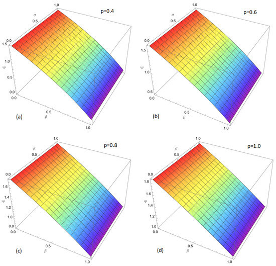
Figure 1.
Approximate solutions of the nonlinear fractional Harry Dym equation using the Laplace Residual Power Series Method (LRPSM) at fractional orders , for . The figure is divided into four subplots, each representing a different fractional order p: (a): The solution for , shown with a rainbow color map where the red color corresponds to higher values of the solution, and the blue color represents lower values. (b): The solution for , following the same rainbow color map, which indicates the evolution of the solution as p increases. (c): The solution for , showing a more refined structure as the fractional order increases further. The color gradient continues to illustrate variations in the solution. (d): The solution for the classical case , which displays the expected behavior for the full-order differential equation. The color map continues to reflect the variation in the solution.
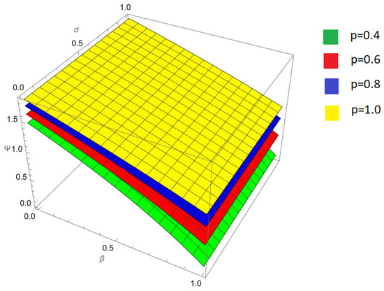
Figure 2.
A comparison between the approximate solutions obtained by the Laplace Residual Power Series Method (LRPSM) and the exact analytical solution of the nonlinear fractional Harry Dym equation at and .
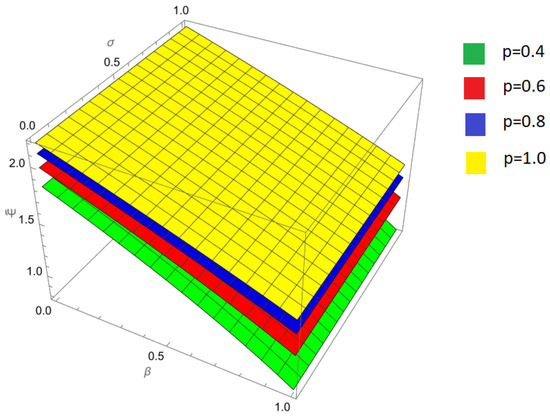
Figure 3.
A comparison between the approximate solutions obtained by the Laplace Residual Power Series Method (LRPSM) and the exact analytical solution of the nonlinear fractional Harry Dym equation at and .
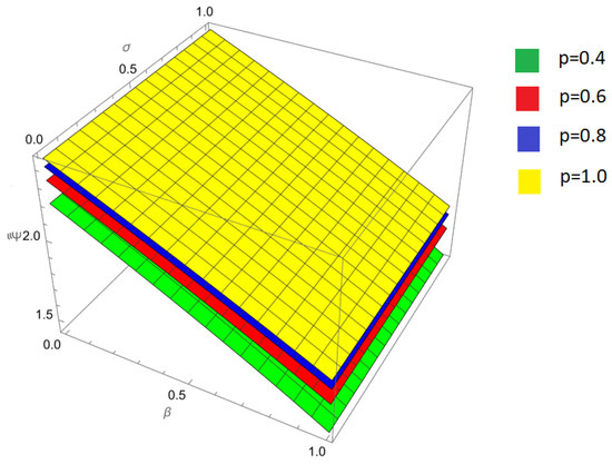
Figure 4.
A comparison between the approximate solutions obtained by the Laplace Residual Power Series Method (LRPSM) and the exact analytical solution of the nonlinear fractional Harry Dym equation at and .
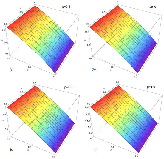
Figure 5.
The approximate solutions of the nonlinear fractional Harry Dym equation obtained using the New Iterative Method (NIM) at fractional orders , for . The figure is divided into four subplots, each representing a different fractional order p: (a): The solution for , shown with a rainbow color map where the red color corresponds to higher values of the solution, and the blue color represents lower values. (b): The solution for , following the same rainbow color map, which indicates the evolution of the solution as p increases. (c): The solution for , showing a more refined structure as the fractional order increases further. The color gradient continues to illustrate variations in the solution. (d): The solution for the classical case , which displays the expected behavior for the full-order differential equation. The **color map** continues to reflect the variation in the solution.
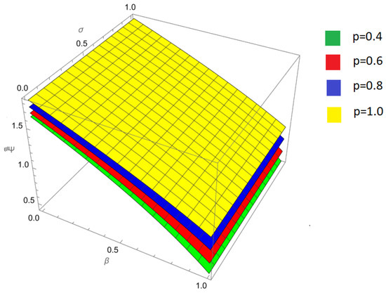
Figure 6.
Comparison of approximate solutions obtained by the New Iterative Method (NIM) with the exact solution of the nonlinear fractional Harry Dym equation for and fractional orders .
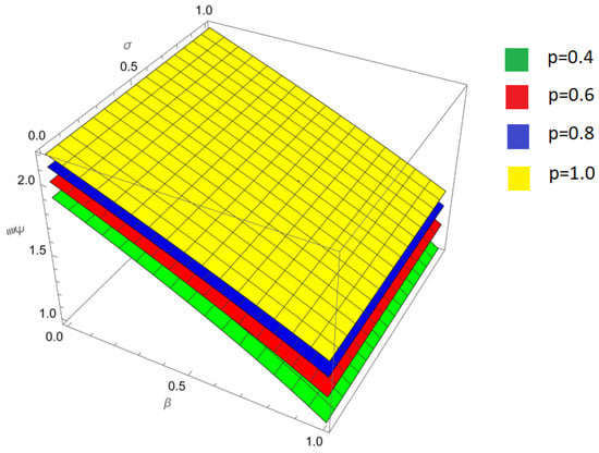
Figure 7.
Comparison of approximate solutions obtained by the New Iterative Method (NIM) with the exact solution of the nonlinear fractional Harry Dym equation and fractional orders .
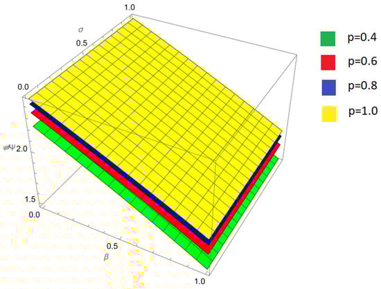
Figure 8.
Comparison of approximate solutions obtained by the New Iterative Method (NIM) with the exact solution of the nonlinear fractional Harry Dym equation and fractional orders .

Table 1.
The comparison of fractional orders of LRPSM and exact with absolute errors .
Table 2.
The comparison of various fractional orders of LRPSM and exact solution with absolute errors for .
Table 3.
Comparison of various fractional orders of LRPSM for exact solution and , .
Table 4.
The comparison of various fractional orders of NIM and exact solution with absolute errors for .
Table 5.
The comparison of various fractional orders of NIM and exact solution with absolute errors for .
Table 6.
The comparison of various fractional orders of NIM and exact solution with absolute errors for .
Table 7.
Comparison of absolute error fractional orders of NIM and LPRSM of example 1 for .
8. Conclusions
In this research, we have designed and validated novel iterative approaches for the challenging domain of nonlinear Harry Dym fractional PDEs. The incorporation of fractional calculus into the mathematical framework has enhanced its stable, enabling the modeling of a broader spectrum of physical processes with more accuracy and realism by considering non-local and memory-dependent effects. In this article, we used the LRPSM and NIM with the Caputo operator to address the complexities of nonlinear Harry Dym PDEs. The LRPSM method has shown to be a valuable numerical tool for estimating solution to nonlinear Harry Dym fractional PDEs. This method, which express the solution in terms of the Laplace operator, is an effective tool for dealing with nonlinearity and fractional derivatives. Furthermore, it has been demonstrated that the Caputo operator allows the proposed NIM to make iterative improvements to the solution of fractional-order differential equations. Due to its high convergence rate and low computational cost, the NIM method shows significant promise as a tool for solving complex problem. When compared to conventional methods, the advantages of the proposed approach in terms of precision and computational efficiency become apparent. Despite the computational complexity of these methods, especially when dealing with large-scale or high-dimensional systems, the proposed approach offers promising accuracy, and its applicability to more complex real-world problems involving multiple variables and boundary conditions may require further optimization for efficiency. As further proof of its adaptability and capacity to address challenges across various scientific domains, these methods have successfully been applied to the solution of nonlinear HDFEs.
For future work, expanding the LRPSM and NIM approach to handle systems with more complex boundary conditions, multi-dimensional spaces, and higher fractional-order derivatives is a promising direction. The potential for these methods to be applied to various types of nonlinear PDEs and incorporated into multidisciplinary contexts should be explored in further research. By investigating how these methods can be used in real-world scenarios, we can gain a better understanding of complex phenomena in fields such as fluid dynamics, combustion, and traffic analysis.
Author Contributions
Conceptualization, M.N. and H.A.; methodology, S.Y.; software, M.N. and S.Y.; validation, T.R.; formal analysis, S.Y.; investigation, T.R.; writing—original draft preparation, M.N.; writing—review and editing, H.A.; visualization, T.R.; supervision, S.Y.; funding acquisition, T.R. All authors have read and agreed to the published version of the manuscript.
Funding
The researchers would like to thank the Deanship of Graduate Studies and Scientific Research at Qassim University for financial support (QU-APC-2025).
Data Availability Statement
The original contributions presented in this study are included in the article. Further inquiries can be directed to the corresponding author.
Acknowledgments
The researchers would like to thank the Deanship of Graduate Studies and Scientific Research at Qassim University for financial support (QU-APC-2025).
Conflicts of Interest
The authors declare that they have no conflicts of interest.
References
- Gharechahi, R.; Arab Ameri, M.; Bisheh-Niasar, M. High order compact finite difference schemes for solving Bratu-type equations. J. Appl. Comput. Mech. 2019, 5, 91–102. [Google Scholar]
- Sharma, J.R.; Kumar, S.; Cesarano, C. An efficient derivative free one-point method with memory for solving nonlinear equations. Mathematics 2019, 7, 604. [Google Scholar] [CrossRef]
- He, J.H.; Wu, X.H. Variational iteration method: New development and applications. Comput. Math. Appl. 2007, 54, 881–894. [Google Scholar] [CrossRef]
- Nadeem, M.; Li, F. Modified Laplace variational iteration method for analytical approach of Klein-Gordon and Sine-Gordon equations. Iran. J. Sci. Technol. Trans. A Sci. 2019, 43, 1933–1940. [Google Scholar] [CrossRef]
- Sadek, L.; Baleanu, D.; Abdo, M.S.; Shatanawi, W. Introducing novel Θ-fractional operators: Advances in fractional calculus. J. King Saud Univ.-Sci. 2024, 36, 103352. [Google Scholar] [CrossRef]
- Sadek, L.; Bataineh, A.S. The general Bernstein function: Application to χ-fractional differential equations. Math. Methods Appl. Sci. 2024, 47, 6117–6142. [Google Scholar] [CrossRef]
- Sadek, L. Controllability, observability, and stability of φ-conformable fractional linear dynamical systems. Asian J. Control 2024, 26, 2476–2494. [Google Scholar] [CrossRef]
- Gul, H.; Ali, S.; Shah, K.; Muhammad, S.; Sitthiwirattham, T.; Chasreechai, S. Application of asymptotic homotopy perturbation method to fractional order partial differential equation. Symmetry 2021, 13, 2215. [Google Scholar] [CrossRef]
- Yusufoglu, E. New solitonary solutions for the MBBM equations using Exp-Function method. Phys. Lett. A 2008, 372, 442–446. [Google Scholar] [CrossRef]
- Sedighi, H.M.; Shirazi, K.H.; Zare, J. An analytic solution of transversal oscillation of quintic non-linear beam with homotopy analysis method. Int. J. Non-Linear Mech. 2012, 47, 777–784. [Google Scholar] [CrossRef]
- Akinyemi, L.; Senol, M.; Iyiola, O.S. Exact solutions of the generalized multidimensional mathematical physics models via sub-equation method. Math. Comput. Simul. 2021, 182, 211–233. [Google Scholar] [CrossRef]
- Abbasbandy, S.; Shirzadi, A. The first integral method for modified Benjamin-Bona-Mahony equation. Commun. Nonlinear Sci. Numer. Simul. 2010, 15, 1759–1764. [Google Scholar] [CrossRef]
- Bekir, A.; Kaplan, M. Exponential rational function method for solving nonlinear equations arising in various physical models. Chin. J. Phys. 2016, 54, 365–370. [Google Scholar] [CrossRef]
- Kaplan, M.; Akbulut, A.; Bekir, A. Exact travelling wave solutions of the nonlinear evolution equations by auxiliary equation method. Z. Naturforschung A 2015, 70, 969–974. [Google Scholar] [CrossRef]
- Kumar, S.; Gomez-Aguilar, J.F. Numerical solution of Caputo-Fabrizio time fractional distributed order reaction-diffusion equation via quasi wavelet based numerical method. J. Appl. Comput. Mech. 2020, 6, 848–861. [Google Scholar]
- Habib, S.; Islam, A.; Batool, A.; Sohail, M.U.; Nadeem, M. Numerical solutions of the fractal foam drainage equation. GEM-Int. J. Geomath. 2021, 12, 7. [Google Scholar] [CrossRef]
- Rawashdeh, M. A new approach to solve the fractional Harry Dym equation using the FRDTM. Int. J. Pure Appl. Math 2014, 95, 553–566. [Google Scholar] [CrossRef]
- Kruskal, M.D.; Moser, J. Dynamical systems, theory and applications. Lect. Notes Phys. 1975, 38, 310–354. [Google Scholar]
- Kumar, S.; Tripathi, M.P.; Singh, O.P. A fractional model of Harry Dym equation and its approximate solution. Ain Shams Eng. J. 2013, 4, 111–115. [Google Scholar] [CrossRef]
- Mokhtari, R. Exact Solutions of the Harry—Dym Equation. Commun. Theor. Phys. 2011, 55, 204. [Google Scholar] [CrossRef]
- Huang, Q.; Zhdanov, R. Symmetries and exact solutions of the time fractional Harry-Dym equation with Riemann–Liouville derivative. Phys. A Stat. Mech. Its Appl. 2014, 409, 110–118. [Google Scholar] [CrossRef]
- Yokus, A.; Gulbahar, S. Numerical solutions with linearization techniques of the fractional Harry Dym equation. Appl. Math. Nonlinear Sci. 2019, 4, 35–42. [Google Scholar] [CrossRef]
- He, J.H. Homotopy perturbation method: A new nonlinear analytical technique. Appl. Math. Comput. 2003, 135, 73–79. [Google Scholar] [CrossRef]
- He, J.H. Recent development of the homotopy perturbation method. Topol. Methods Nonlinear Anal. 2008, 31, 205–209. [Google Scholar]
- Singh, M.; Gupta, P.K. Homotopy perturbation method for time-fractional shock wave equation. Adv. Appl. Math. Mech. 2011, 3, 774–783. [Google Scholar] [CrossRef]
- Li, F.; Nadeem, M. He-Laplace method for nonlinear vibration in shallow water waves. J. Low Freq. Noise Vib. Act. Control 2019, 38, 1305–1313. [Google Scholar] [CrossRef]
- Nadeem, M.; Li, F. He–Laplace method for nonlinear vibration systems and nonlinear wave equations. J. Low Freq. Noise Vib. Act. Control 2019, 38, 1060–1074. [Google Scholar] [CrossRef]
- Liaqat, M.I.; Okyere, E. Comparative Analysis of the Time-Fractional Black-Scholes Option Pricing Equations (BSOPE) by the Laplace Residual Power Series Method (LRPSM). J. Math. 2023, 2023, 6092283. [Google Scholar] [CrossRef]
- Shafee, A.; Alkhezi, Y.; Shah, R. Efficient Solution of Fractional System Partial Differential Equations Using Laplace Residual Power Series Method. Fractal Fract. 2023, 7, 429. [Google Scholar] [CrossRef]
- Albalawi, W.; Shah, R.; Nonlaopon, K.; El-Sherif, L.S.; El-Tantawy, S.A. Laplace Residual Power Series Method for Solving Three-Dimensional Fractional Helmholtz Equations. Symmetry 2023, 15, 194. [Google Scholar] [CrossRef]
- Luo, X.; Nadeem, M. Laplace residual power series method for the numerical solution of time-fractional Newell–Whitehead–Segel model. Int. J. Numer. Methods Heat Fluid Flow 2023, 33, 2377–2391. [Google Scholar] [CrossRef]
- Singh, B.K.; Agrawal, S.; Singh, N. Revised residual power series method in Laplacian space for space-time fractional PDEs with proportional delayed arguments. Math. Methods Appl. Sci. 2023, 48, 7495–7513. [Google Scholar] [CrossRef]
- Batiha, B. Solving one species Lotka–volterra equation by the new iterative method (NIM). WSEAS Trans. Math. 2023, 22, 324–329. [Google Scholar] [CrossRef]
- Batiha, B.; Ghanim, F.; Batiha, K. Application of the New Iterative Method (NIM) to the Generalized Burgers–Huxley Equation. Symmetry 2023, 15, 688. [Google Scholar] [CrossRef]
- Batiha, B.; Al-khateeb, A.; Zureigat, H. Improving Numerical Solutions for the Generalized Huxley Equation: The New Iterative Method (NIM). Appl. Math 2023, 1, 427–493. [Google Scholar]
- Batiha, B.; Heilat, A.S.; Ghanim, F. Closed-Form Solutions for Cauchy-Euler Differential Equations through the New Iterative Method (NIM). Appl. Math 2023, 17, 459–467. [Google Scholar]
- Jafarian, A. On the Solution of Volterra-Fredholm Integro-Differential Equation by Using New Iterative Method. Int. J. Ind. Math. 2023, 15, 21–26. [Google Scholar]
- Ghareeb, S.M.; Arif, G.E.; Jumaa, B.F. Modified New Iterative Method for Solving Systems of Nonlinear Volterra Integral Equations of the Second Kind. J. Nat. Appl. Sci. URAL 2023, 1, 85–93. [Google Scholar]
- Nawaz, R.; Iqbal, A.; Bakhtiar, H.; Alhilfi, W.A.; Fewster-Young, N.; Ali, A.H.; Poțclean, A.D. A New Extension of Optimal Auxiliary Function Method to Fractional Non-Linear Coupled ITO System and Time Fractional Non-Linear KDV System. Axioms 2023, 12, 881. [Google Scholar] [CrossRef]
- Khater, M.M. Wave propagation analysis in the modified nonlinear time fractional harry dym equation: Insights from khater ii method and b-spline schemes. Mod. Phys. Lett. B 2024, 38, 2450288. [Google Scholar] [CrossRef]
- Khater, M.M. Dynamics of nonlinear time fractional equations in shallow water waves. Int. J. Theor. Phys. 2024, 63, 92. [Google Scholar] [CrossRef]
- Alshammari, S.; Iqbal, N.; Yar, M. Analytical Investigation of Nonlinear Fractional Harry Dym and Rosenau-Hyman Equation via a Novel Transform. J. Funct. Spaces 2022, 2022, 8736030. [Google Scholar] [CrossRef]
- O’Regan, D.; Aderyani, S.R.; Saadati, R.; Inc, M. Soliton Solution of the Nonlinear Time Fractional Equations: Comprehensive Methods to Solve Physical Models. Axioms 2024, 13, 92. [Google Scholar] [CrossRef]
- Altuijri, R.; Abdel-Aty, A.H.; Nisar, K.S.; Khater, M.M. Exploring plasma dynamics: Analytical and numerical insights into generalized nonlinear time fractional Harry Dym equation. Mod. Phys. Lett. B 2024, 38, 2450264. [Google Scholar] [CrossRef]
- Biswas, S.; Ghosh, U. Formulation of conformable time fractional differential equation and q-HAM solution comparison with ADM. J. Phys. Soc. Jpn. 2022, 91, 044007. [Google Scholar] [CrossRef]
- Buryachenko, K.; Chugunova, M.; Kolomoitsev, Y. Approximation methods and analytical modeling using partial differential equations. Front. Appl. Math. Stat. 2025, 11, 1584781. [Google Scholar] [CrossRef]
- Nagaraja, M.; Chethan, H.B.; Shivamurthy, T.R.; Shah, M.A.; Prakasha, D.G. Semi-analytical approach for the approximate solution of Harry Dym and Rosenau–Hyman equations of fractional order. Res. Math. 2024, 11, 2401662. [Google Scholar] [CrossRef]
- ÇULHA ÜNAL, S. Approximate solutions of the fractional Harry Dym equation. Sigma J. Eng. Nat. Sci. 2024, 42, 1604–1611. [Google Scholar] [CrossRef]
- Assabaai, M.A. Numerical solution of the Harry Dym equation using Chebyshev spectral method via Lie group method. J. Phys. Conf. Ser. 2021, 1900, 012004. [Google Scholar] [CrossRef]
- El-Ajou, A. Adapting the Laplace transform to create solitary solutions for the nonlinear time-fractional dispersive PDEs via a new approach. Eur. Phys. J. Plus 2021, 136, 229. [Google Scholar] [CrossRef]
- Daftardar-Gejji, V.; Jafari, H. An iterative method for solving nonlinear functional equations. J. Math. Anal. Appl. 2006, 316, 753–763. [Google Scholar] [CrossRef]
- Bhalekar, S.; Daftardar-Gejji, V. Convergence of the new iterative method. Int. J. Differ. Equ. 2011, 2011, 989065. [Google Scholar] [CrossRef]
- Nadeem, M.; Li, Z.; Alsayyad, Y. Analytical approach for the approximate solution of harry dym equation with caputo fractional derivative. Math. Probl. Eng. 2022, 1, 4360735. [Google Scholar] [CrossRef]
- Alquran, M.; Ali, M.; Alsukhour, M.; Jaradat, I. Promoted residual power series technique with Laplace transform to solve some time-fractional problems arising in physics. Results Phys. 2020, 19, 103667. [Google Scholar] [CrossRef]
Disclaimer/Publisher’s Note: The statements, opinions and data contained in all publications are solely those of the individual author(s) and contributor(s) and not of MDPI and/or the editor(s). MDPI and/or the editor(s) disclaim responsibility for any injury to people or property resulting from any ideas, methods, instructions or products referred to in the content. |
© 2025 by the authors. Licensee MDPI, Basel, Switzerland. This article is an open access article distributed under the terms and conditions of the Creative Commons Attribution (CC BY) license (https://creativecommons.org/licenses/by/4.0/).