Abstract
This study focuses on approximating continuous functions using Frobenius–Euler–Simsek polynomial analogues of Szász operators. Test functions and central moments are computed to study convergence uniformly, approximation order by these operators. Next, we investigate approximation order uniform convergence via Korovkin result and the modulus of smoothness for functions in continuous functional spaces. A Voronovskaja theorem is also explored approximating functions which belongs to the class of function having first and second order continuous derivative. Further, we discuss numerical error and graphical analysis. In the last, two dimensional operators are constructed to discuss approximation for the class of two variable continuous functions.
Keywords:
Voronovskaja theorem; mathematical operators; rate of convergence; Frobenius polynomials; modulus of continuity; approximation algorithms MSC:
41A10; 41A28; 41A25; 41A35; 41A36
1. Introduction and Preliminaries
Bernstein (1912) [1] introduced a sequence of polynomials to present the simplest proof of an elegant theorem due to Weierstrass (1885) [2] which is termed as the Weierstrass approximation theorem in terms of the binomial probability distribution, as follows:
Define for . It is well established that the sequence of operators converges uniformly to ℏ on for every bounded function ℏ, i.e., . In recent developments, operator theory has emerged as a powerful tool, establishing strong interdisciplinary connections across various fields of science, including engineering and medical sciences. Notable applications can be found in areas such as robotics, computer-aided geometric design (CAGD), and the modeling of diseases like HIV, among others [3,4,5,6,7,8]. Over the past decade, numerous mathematicians have proposed various modifications of the operators defined in (1) in order to enhance their flexibility in approximation properties on both bounded and unbounded intervals within different functional spaces, for example, Özger et al. [9,10], Aslan et al. [11,12], Ayman et al. [13,14], Mohiuddine et al. [15,16], Mursaleen et al. [17,18], Khan et al. [19], Nasiruzzaman [20], Braha et al. [21], Rao et al. [22,23,24], Çetin et al. [25,26]. Numerous researchers have developed significant literature in the field of approximation theory, such as [27,28,29,30,31,32,33,34,35,36,37,38,39,40,41]. In the context of polynomial classes, which constitute an active area of research within the broader field of special functions, we recall a class of polynomials introduced by Simsek [42], known as the Frobenius Simsek Euler type polynomials andnumbers denoted by . Frobenius–Euler polynomials possess rich symmetric properties [43], often expressed through binomial expansions and translation identities. These symmetries simplify computations and reveal deep structural relationships among the polynomials. Such properties have important applications in combinatorics, number theory, and special functions connected with the generating function, such as:
As , one yields Frobenious–Simsek–Euler–type numbers as follows:
Setting in above relation, one obtains the following:
For detailed information and application regarding Frobenius–Euler–Simsek-type numbers, see [44,45]. Motivated by the aforementioned developments, We propose a new formulation of Szász–Chlodowsky operators incorporating Frobenius–Şimşek–Euler–type numbers, defined as:
Lemma 1
Lemma 2.
Based on the generating function given in (3), we derive the following:
Proof.
Applying Lemma (1), Lemma (2) can be established by taking and replacing y with . □
Lemma 3.
Let , . Then, one yields:
Proof.
To prove Lemma (3) in view of given in (4), we have the following:
For ,
For , we yield the following:
In the light of Equation (2), we yield:
For ,
Based on Lemma (2), we yield the following:
□
Lemma 4.
Let . Then, for the sequence of operators given by (4), the following properties hold:
Proof.
Using (4) and its linearity property, we yield:
In the light of Lemma 3, we arrived required Lemma. □
Remark 1.
The operators introduced in (4) are found as positive, i.e., for , .
Remark 2.
The operators introduced in (4) are found as linear, i.e., for every and , we yield the following:
This manuscript investigates the approximation results for the sequence of operators defined in (4). It addresses several fundamental aspects, including uniform convergence, pointwise convergence, and theorem due Voronovskaja. Furthermore, a bivariate sequence of operators is constructed, and their uniform rate of approximation as well as the order of approximation are analyzed. Finally, the study explores direct approximation results using these operators in various functional spaces.
2. Voronovskaja-Type Theorem and Order of Approximation
Definition 1
(See [46]). Let (a space of continuous and bounded functions). Then, modulus of smoothness is given as follows:
and
Theorem 1.
Let be introduced in (4) and for all . Then, on a bounded subset of where ⇉ depicts that the convergence is uniform.
Proof.
According to the theorem due to Korovkin [47], it is only required to demonstrate that:
On each compact subset of uniformly, and applying Lemma (3), one obtain the required proof of this theorem.
□
The next approximation result involves the investigation of the order of approximation (4) using modulus of smoothness given in (6), as follows:
Theorem 2.
Proof.
Using (4), we get
By applying the Cauchy–Schwarz inequality, we have
On choosing , we yield the following:
Thus, we conclude the proof of above Theorem. □
We now state the Voronovskaja result for functions havingfirst and second ordered continuous derivatives, employing the sequences in (4), as:
Theorem 3.
Let converge as and Then, we receive the following:
Proof.
For function approximation, first, we recall the expansion of the Taylor series:
where is a remainder term and with . We apply given in Equations (4)
Taking limits both the sides (9), we get following result:
Using the inequality due to Cauchy–Schwarz inequality:
Using Equations (10) and (11), Lemma (4), and , we derive the following:
Hence we arrived the desired result. □
3. Convergence Analysis via Numerical and Graphical Methods
This section, we focus on examination of the convergence behavior of the operators defined in (4). The analysis is conducted for different values of m, specifically , , and . The convergence behavior is visualized in Figure 1, which highlights the impact of increasing m on the operator’s performance. Furthermore, the approximation error for these cases is illustrated in Figure 2, providing a clear depiction of the error trends.
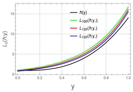
Figure 1.
Convergence behavior for .
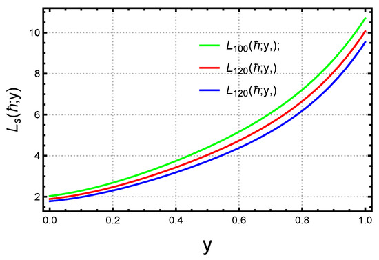
Figure 2.
Error approximation .
To quantitatively evaluate the convergence, we compute the numerical errors using the following formula:
where is defined as follows:
The computed numerical errors are presented in Table 1. These errors are crucial for understanding the approximation accuracy of the operators for different values of m and demonstrate the rate of convergence as m increases.

Table 1.
The approximation error of the operators with respect to .
Significance of Numerical Analysis
The numerical analysis confirms the theoretical results and shows how the operators behave in practice. By calculating the errors for various y-values, we can understand how well the operators approximate the target function . This is important for applications where accuracy is key.
4. Results on Local Approximation
Let us recall the definition of the Lipschitz-type space [48], given by:
where , and .
Theorem 4.
Let be the sequences of the operator given by (4). Then, for , one has the following:
choosing , and .
Proof.
Given and , one yields the following:
Since , for each , one has
This means that Theorem 4 holds for . Next, for , using Hölder’s inequality with and , we get the following:
Since , for all , we yields
Thus, we have proved Theorem 4. □
5. A Bivariate Frobenius–Şimşek–Euler Polynomial Representation of Szász Operators
In this part, we construct the bivariate form of the operators described in (4). And, let denote the category of functions that are continuous on equipped with the supremum norm:
For all and , we introduce a bivariate version of as follows:
where
with
and Let be a sequence of positive, increasing real numbers. The sequence satisfies the following conditions:
- ,
- for .
Let with . We define the two-dimensional test functions as , and the central moments as .
Lemma 5.
Given , the operator from Equation (15), and the test functions , we have the following:
Proof.
The above lemma is proved using the linearity property and Lemma (3) as follows:
□
Lemma 6.
For for such that , we have the following equalities:
Proof.
By Lemma 5 and the linearity property, the desired result follows easily. □
6. Error Bounds and Approximation Order
To study the rate of convergence of the operators defined in (15), we make use of the result established by Volkov [49], which offers an effective framework for analyzing the convergence behavior, as outlined below:
Theorem 5.
Consider compact intervals I and J on the real line. Let , and define as linear positive operators.
If
and
uniformly on . Then, for any , the sequence converges uniformly to ℏ.
Theorem 6.
Let be the test functions restricted on . If
and
uniformly on . Then,
uniformly for all .
Proof.
In the light of Lemma 5, it is evident for
For , , we obtain the following:
Similarly,
Using Lemma (5), we obtain:
In the direction of Theorem 5, we establish the desired result. □
In the final result, we address the order of approximation for the sequence of operators defined in (15) as follows:
Theorem 7.
([50]). Let be a linear positive operator. Then, for any , any , and any , the following inequality holds:
Theorem 8.
For and , , and , one has the following:
where and .
Proof.
From Theorem 7, we have the following:
Selecting
and , we arrive at the required result. □
7. Bivariate Operators: Graphical and Tabular Representations
To verify the convergence of the operator defined in (15), we perform both graphical and numerical analyses. For this purpose, we consider the following test function:
The corresponding results are displayed in Figure 3.
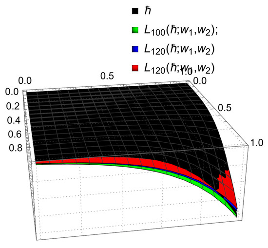
Figure 3.
Convergence of operator for .
Furthermore, to evaluate the error approximation, we utilize the formula:
The error is examined for various values of and , specifically and 140. The corresponding error approximations are illustrated graphically in Figure 4 and listed in Table 2. These representations together offer insights into the accuracy and behavior of the operator as the values of and increase, highlighting the convergence of the operator to the target function .
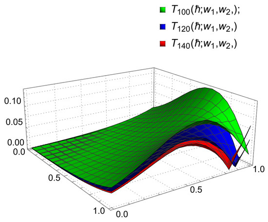
Figure 4.
Error approximation .
Table 2.
Error approximation table .
8. Conclusions
In conclusion, this research explores the approximation of continuous functions using Frobenius–Euler–Simsek polynomial analogues of Szász operators. The study demonstrates uniform convergence, approximation order, and the application of Korovkin and modulus of continuity for continuous functional spaces. A Voronovskaja-type theorem is presented for functions with continuous first and second derivatives. Numerical and graphical analyses, including the construction of a bivariate sequence, further illustrate the accuracy and efficiency of the operators in approximating both univariate and bivariate continuous functions. The findings contribute valuable insights for applications requiring high precision.
Author Contributions
Conceptualization, M.F.; Methodology, N.R.; Software, M.R.; Writing—original draft, N.R.; Writing—review & editing, M.F. and M.R. All authors have read and agreed to the published version of the manuscript.
Funding
The APC was funded by the Deanship of Graduate Studies and Scientific Research at Qassim University for financial support (QU-APC-2025).
Data Availability Statement
Data are contained within the article.
Acknowledgments
The Researchers would like to thank the Deanship of Graduate Studies and Scientific Research at Qassim University for financial support (QU-APC-2025).
Conflicts of Interest
The authors declare no conflicts of interest.
References
- Bernstein, S.N. Démonstration du théorème de Weierstrass fondée sur le calcul de probabilités. Commun. Soc. Math. Kharkow. 1913, 13, 1–2. [Google Scholar]
- Weierstrass, K. Über die analytische Darstellbarkeit sogenannter willkürlicher Functionen einer reellen Veränderlichen. Sitzungsberichte KöNiglichen PreußIschen Akad. Wiss. Berl. 1885, 2, 633–639. [Google Scholar]
- Agyuz, E. Onthe convergence properties of generalized Szász–Kantorovich type operators involving Frobenious–Euler–Simsek-type polynomials. Aims Math. 2024, 9, 28195–28210. [Google Scholar] [CrossRef]
- Khan, K.; Lobiyal, D.K. Bézier curves based on Lupăs (p, q)-analogue of Bernstein functions in CAGD. Comput. Appl. Math. 2017, 317, 458–477. [Google Scholar] [CrossRef]
- Khan, K.; Lobiyal, D.K.; Kilicman, A. Bézier Curves and Surfaces Based on Modified Bernstein Polynomials. Azerb. J. Math. 2019, 9, 3–21. [Google Scholar]
- Izadbakhsh, A.; Kalat, A.A.; Khorashadizadeh, S. Observer-based adaptive control for HIV infection therapy using the Baskakov operator. Biomed. Signal Process. Control 2021, 65, 102343. [Google Scholar] [CrossRef]
- Uyan, H.; Aslan, A.O.; Karateke, S.; Büyükyazıcı, İ. Interpolation for neural network operators activated with a generalized logistic-type function. J. Inequalities Appl. 2024, 2024, 125. [Google Scholar] [CrossRef]
- Zhang, Q.; Mu, M.; Wang, X. A Modified Robotic Manipulator Controller Based on Bernstein-Kantorovich-Stancu Operator. Micromachines 2022, 14, 44. [Google Scholar] [CrossRef]
- Özger, F. Weighted statistical approximation properties of univariate and bivariate λ-Kantorovich operators. Filomat 2019, 33, 3473–3486. [Google Scholar] [CrossRef]
- Özger, F.; Ansari, K.J. Statistical convergence of bivariate generalized Bernstein operators via four-dimensional infinite matrices. Filomat 2022, 36, 507–525. [Google Scholar] [CrossRef]
- Aslan, R. Rate of approximation of blending type modified univariate and bivariate λ-Schurer-Kantorovich operators. Kuwait J. Sci. 2024, 51, 100168. [Google Scholar] [CrossRef]
- Aslan, R. Approximation properties of univariate and bivariate new class-Bernstein–Kantorovich operators and its associated GBS operators. Comp. Appl. Math. 2023, 42, 34. [Google Scholar] [CrossRef]
- Ayman-Mursaleen, M.; Heshamuddin, M.; Rao, N.; Sinha, B.K.; Yadav, A.K. Hermite polynomials linking Szász–Durrmeyer operators. Comp. Appl. Math. 2024, 43, 223. [Google Scholar] [CrossRef]
- Ayman-Mursaleen, M.; Rao, N.; Rani, M.; Kilicman, A.; Al-Abied, A.A.H.A.; Malik, P. A Note on Approximation of Blending Type Bernstein–Schurer–Kantorovich Operators with Shape Parameter α. J. Math. 2023, 2023, 5245806. [Google Scholar] [CrossRef]
- Mohiuddine, S.A.; Acar, T.; Alotaibi, A. Construction of a new family of Bernstein-Kantorovich operators. Math. Methods Appl. Sci. 2017, 40, 7749–7759. [Google Scholar] [CrossRef]
- Mohiuddine, S.A.; Ahmad, N.; Özger, F.; Alotaibi, A.; Hazarika, B. Approximation by the parametric generalization of Baskakov–Kantorovich operators linking with Stancu operators. Iran. J. Sci. Technol. Trans. 2021, 45, 593–605. [Google Scholar] [CrossRef]
- Mursaleen, M.; Ansari, K.J.; Khan, A. Approximation properties and error estimation of q-Bernstein shifted operators. Numer. Algorithms 2020, 84, 207–227. [Google Scholar] [CrossRef]
- Mursaleen, M.; Naaz, A.; Khan, A. Improved approximation and error estimations by King type (p, q)-Szász-Mirakjan Kantorovich operators. Appl. Math. Comput. 2019, 348, 2175–2185. [Google Scholar] [CrossRef]
- Khan, A.; Mansoori, M.; Khan, K.; Mursaleen, M. Phillips-type q-Bernstein operators on triangles. J. Funct. Spaces 2021, 2021, 6637893. [Google Scholar] [CrossRef]
- Nasiruzzaman, M. Approximation properties by Szász–Mirakjan operators to bivariate functions via Dunkl analogue. Iran. J. Sci. Technol. Trans. 2011, 45, 259–269. [Google Scholar] [CrossRef]
- Braha, N.L.; Loku, V.; Mansour, T.; Mursaleen, M. A new weighted statistical convergence and some associated approximation theorems. Math. Methods Appl. Sci. 2022, 45, 5682–5698. [Google Scholar] [CrossRef]
- Rao, N.; Farid, M.; Ali, R.A. Study of Szász–Durremeyer-Type Operators Involving Adjoint Bernoulli Polynomials. Mathematics 2024, 12, 3645. [Google Scholar] [CrossRef]
- Rao, N.; Farid, M.; Raiz, M. Symmetric Properties of λ-Szász Operators Coupled with Generalized Beta Functions and Approximation Theory. Symmetry 2024, 16, 1703. [Google Scholar] [CrossRef]
- Rao, N.; Farid, M.; Raiz, M. Approximation Results: Szász– Kantorovich Operators Enhanced by Frobenius–Euler–Type Polynomials. Axioms 2025, 14, 252. [Google Scholar] [CrossRef]
- Çetin, N. Approximation and geometric properties of complex α-Bernstein operator. Results Math. 2019, 74, 40. [Google Scholar] [CrossRef]
- Çetin, N.; Radu, V.A. Approximation by generalized Bernstein-Stancu operators. Turk. J. Math. 2019, 43, 2032–2048. [Google Scholar] [CrossRef]
- Arı, D.A.; Yılmaz, G.U. A Note On Kantorovich Type Operators Which Preserve Affine Functions. Fundam. J. Math. Appl. 2024, 1, 53–58. [Google Scholar]
- Çiçek, H.; İzgi, A. Approximation by Modified Bivariate Bernstein-Durrmeyer and GBS Bivariate Bernstein-Durrmeyer Operators on a Triangular Region. Fundam. J. Math. Appl. 2022, 5, 135–144. [Google Scholar] [CrossRef]
- Aslan, R. Some Approximation Results on λ–Szász-Mirakjan-Kantorovich Operators. Fundam. J. Math. Appl. 2021, 4, 150–158. [Google Scholar] [CrossRef]
- Baytunç, E.; Aktuğlu, H.; Mahmudov, N. A New Generalization of Szász-Mirakjan Kantorovich Operators for Better Error Estimation. Fundam. J. Math. Appl. 2023, 6, 194–210. [Google Scholar] [CrossRef]
- Qazza, A.; Bendib, I.; Hatamleh, R.; Saadeh, R.; Ouannas, A. Finite-time synchronization control for fractional-order reaction–diffusion systems with Neumann boundary conditions. Partial. Diff. Equations Appl. Math. 2024, 13, 101125. [Google Scholar]
- Qazza, A.; Bendib, I.; Hatamleh, R.; Saadeh, R.; Ouannas, A. Dynamics of the Gierer–Meinhardt reaction–diffusion system: Insights into finite-time stability and control strategies. Partial. Differ. Equ. Appl. Math. 2025, 13, 101142. [Google Scholar] [CrossRef]
- Batiha, I.M.; Ogilat, O.; Bendib, I.; Ouannas, A.; Jebril, I.H.; Anakira, N. Finite-time dynamics of the fractional-order epidemic model: Stability, synchronization, and simulations. Chaos, Solitons Fractals X 2024, 130, 100118. [Google Scholar] [CrossRef]
- Sadek, L.; Baleanu, D.; Abdo, M.S.; Shatanawi, W. Introducing novel θ-fractional operators: Advances in fractional calculus. J. King Saud-Univ.-Sci. 2024, 36, 103352. [Google Scholar] [CrossRef]
- Sadek, L. Controllability, observability, and stability of ϕ-conformable fractional linear dynamical systems. Asian J. Control. 2024, 26, 2476–2494. [Google Scholar] [CrossRef]
- Sadek, L.; Lazar, T.A. On Hilfer cotangent fractional derivative and a particular class of fractional problems. Aims Math. 2023, 8, 28334–28352. [Google Scholar] [CrossRef]
- Sadek, L.; Jarad, F. The general Caputo–Katugampola fractional derivative and numerical approach for solving the fractional differential equations. Alex. Eng. J. 2025, 121, 539–557. [Google Scholar] [CrossRef]
- Hou, Q.; Li, Y.; Singh, V.P.; Sun, Z. Physics-informed neural network for diffusive wave model. J. Hydrol. 2024, 637, 131261. [Google Scholar] [CrossRef]
- Feng, G.; Yu, S.; Wang, T.; Zhang, Z. Discussion on the Weak Equivalence Principle for a Schwarzschild Gravitational Field Based on the Light-Clock Model. Ann. Phys. 2025, 473, 169903. [Google Scholar] [CrossRef]
- Sun, W.; Jin, Y.; Lü, G. Genuine Multipartite Entanglement from a Thermodynamic Perspective. Phys. Rev. A 2024, 109, 042422. [Google Scholar] [CrossRef]
- Lenze, B. On Lipschitz type maximal functions and their smoothness spaces. Nederl. Akad. Indag. Math. 1988, 50, 53–63. [Google Scholar] [CrossRef]
- Simsek, Y. Applications of constructed new families of generating-type functions interpolating new and known classes of polynomials and numbers. Math. Methods Appl. Sci. 2021, 44, 11245–11268. [Google Scholar] [CrossRef]
- Araci, S.; Duran, U.; Acikgoz, M. Symmetric Identities Involving q-Frobenius-Euler Polynomials under Sym (5). Turk. J. Anal. Number Theory 2015, 3, 90–93. [Google Scholar] [CrossRef]
- Kucukoglu, I. Generating functions for multiparametric Hermite-based Peters-type Simsek numbers and polynomials in several variables. Montes Taurus J. Pure Appl. Math. 2024, 6, 217–238. [Google Scholar]
- Kucukoglu, I.; Simsek, Y. Identities and relations on the q-Apostol type Frobenius-Euler numbers and polynomials. J. Korean Math. Soc. 2019, 56, 265–284. [Google Scholar]
- DeVore, R.A.; Lorentz, G.G. Constructive Approximation; Springer: Berlin, Germany, 1993. [Google Scholar]
- Altomare, F.; Campiti, M. Korovkin-type approximation theory and its applications. De Gruyter Ser. Stud. Math. 1994, 17, 266–274. [Google Scholar]
- Özarslan, M.A.; Aktuğlu, H. Local approximation for certain King type operators. Filomat 2013, 27, 173–181. [Google Scholar] [CrossRef]
- Volkov, V.I. On the convergence of sequences of linear positive operators in the space of continuous functions of two variables. Dokl. Akad. Nauk SSSR (NS) 1957, 115, 17–19. (In Russian) [Google Scholar]
- Stancu, F. Aproximarca Funcţiilor de Două şi Mai Multe Variabile Prin şiruri de Operatori Liniari şi Pozitivi. Ph.D. Thesis, Babeṣ-Bolyai University, Cluj-Napoca, Romania, 1984. (In Romanian). [Google Scholar]
Disclaimer/Publisher’s Note: The statements, opinions and data contained in all publications are solely those of the individual author(s) and contributor(s) and not of MDPI and/or the editor(s). MDPI and/or the editor(s) disclaim responsibility for any injury to people or property resulting from any ideas, methods, instructions or products referred to in the content. |
© 2025 by the authors. Licensee MDPI, Basel, Switzerland. This article is an open access article distributed under the terms and conditions of the Creative Commons Attribution (CC BY) license (https://creativecommons.org/licenses/by/4.0/).