The Radial Symmetry and Monotonicity of Solutions of Fractional Parabolic Equations in the Unit Ball

Abstract

We use the method of moving planes to prove the radial symmetry and monotonicity of solutions of fractional parabolic equations in the unit ball. Since the fractional Laplacian operator is a linear operator, we investigate the maximal regularity of nonlocal parabolic fractional Laplacian equations in the unit ball. The maximal regularity of nonlocal parabolic fractional Laplacian equations guarantees the existence of solutions in the unit ball. Based on these conditions, we first establish a maximum principle in a parabolic cylinder, and the principles provide a starting position to apply the method of moving planes. Then, we consider the fractional parabolic equations and derive the radial symmetry and monotonicity of solutions in the unit ball.

1. Introduction

In this paper, we consider nonlinear equations involving the fractional parabolic equation in the unit ball

$$\begin{array}{c}\hfill {\displaystyle \frac{\partial u}{\partial t}}(x,t)+{(-\Delta )}^{s}u(x,t)=f(t,|x|,u)\end{array}$$

(1)

with

$$\begin{array}{ccc}\hfill {(-\Delta )}^{s}u(x,t)& \equiv & C_{n,s}P.V.{\int }_{{\mathbb{R}}^n}{\displaystyle \frac{u(x,t)-u(y,t)}{{|x-y|}^{n+2s}}}dy\hfill \\ & \equiv & C_{n,s}\underset{\epsilon \to 0^{+}}{lim}{\int }_{{\mathbb{R}}^n\setminus B_{\epsilon }\left(x\right)}{\displaystyle \frac{u(x,t)-u(y,t)}{{|x-y|}^{n+2s}}}dy,\hfill \end{array}$$

(2)

for any real number $0<s<1$, where $C_{n,s}$ is a normalization positive constant depending on n and s, and $P.V.$ stands for the Cauchy principal value.

In order to understand the integral in (2), we require that $u\in {\mathcal{L}}_{2s}\cap C_{loc}^{1,1}$ with

$$\begin{array}{c}\hfill {\mathcal{L}}_{2s}\equiv \left\{u:{\mathbb{R}}^n\to \mathbb{R}|{\int }_{{\mathbb{R}}^n}{\displaystyle \frac{\left|u\right(x,t\left)\right|}{1+{\left|x\right|}^{n+2s}}}dx<+\infty \right\}.\end{array}$$

In contrast to the usual differential operators, the fractional Laplacian is a nonlocal operator, meaning that its value at a point depends on the values of the function in the whole space. This nonlocality gives rise to a number of mathematical properties that make the fractional Laplacian an important tool for modeling nonlocal phenomena, and has gained much attention in recent years, with a lot of researchers studying equations involving the fractional Laplacian (e.g., Cabré & Cinti, 2014; Caffarelli & Silvestre, 2007; Felmer & Wang, 2014; Musina & Nazarov, 2014; Chen et al., 2015; Cabré & Sire, 2015 [1,2,3,4,5,6]; and references therein). During the past two decades, researchers have developed several methods for studying the lower-order fractional operators with $s\in (0,1)$. Notably, the extension method (Caffarelli & Silvestre, 2007) [2] and the integral method (Chen & Li, [7]) have produced fruitful outcomes. To our knowledge, the extension method cannot be applied to higher-order fractional problems with $s>1$ due to technical limitations. In contrast, applying the integral method requires imposing additional constraints on the integrability of solutions; consequently, the integral method also loses its effectiveness. In 2017, Chen et al. (2017) [8] introduced a direct method of moving planes for the fractional Laplacian, to avoid circumventing the issue and investigate nonlocal problems directly, they applied it to obtain the symmetry, existence/nonexistence, and regularity properties of solutions of various problems (e.g., Caffarelli et al., [9,10,11]; and references therein). The method of moving planes was first introduced by A. D. Alexandrov (1950s) to prove the celebrated Soap Bubble Theorem. Since its inception, the method has been refined and extended by numerous mathematicians, including Serrin (1971) [12], who applied it to establish symmetry results for elliptic equations. In recent years, the method has been adapted for nonlocal problems, such as in the direct method of moving planes (e.g., Chen et al., 2019 [13]), which arise naturally in models of anomalous diffusion, Lévy flights, and image processing. This adaptation has facilitated the study of nonlinear problems (e.g., Cai & Ma, 2018; Chen & Li, 2018; Chen et al., 2017 [14,15,16]).

In our paper, we use the direct method of moving planes (Chen et al., 2017 [8]) to study the radial symmetry and monotonicity of solutions of fractional parabolic equations in the unit ball. Du and Wang (2023) [17] use the direct method of moving planes to prove the monotonicity of solutions of equations involving a nonlocal Monge–Ampère operator; however, they only discuss how to address problems when restricting variables solely to the half-space, since the nonlocal fractional operator generates the semi-group in ${\mathbb{R}}_{+}^n\times \mathbb{R}$. We generalize the variables to the unit ball. When the variables are not restricted to a half-space, ensuring the existence of solutions within this framework requires preserving maximal regularity. To achieve this, we adopt the method proposed by Liu (2024) in [18], which involves controlling the norm of the spatial operator to be less than 1. However, since the fractional Laplacian is nonlocal, the challenge lies in how to enforce such a norm constraint. Conventionally, one might assume uniform convergence and boundedness of the solution u (e.g., $\left|u\right(x,t\left)\right|\le 1$), as in Chen et al. (2020) [19]. In contrast, our paper boldly relaxes this assumption, requiring only that u converges almost everywhere—a key innovation that distinguishes our work from the existing literature. Meanwhile, our paper also employs a localization procedure by restricting the problem to specific local subdomains of the domain of interest. This approach transforms a global partial differential equation problem into locally tractable subproblems, thereby simplifying analysis or computation. For instance, in Section 3 of the paper, we utilize the Fourier transform to decompose the partial differential equation into distinct frequency components and achieve localization by truncating certain frequency ranges. Similarly, in Section 5, we confine the problem to a specific region using a cut-off function, effectively localizing the analysis.

The fractional Laplacian, as a nonlocal operator, requires values from the entire domain to determine its values on the boundary. Consequently, there is currently a lack of literature addressing boundary-value problems for partial differential equations involving the fractional Laplacian. Although our study incorporates an investigation into maximal regularity, we still adhere to the common assumption, adopted in the majority of existing works, of imposing homogeneous (zero) boundary conditions. If we consider $u{\mid }_{\partial B_1\left(0\right)}\not\equiv 0$, we have to consider the boundary conditions ${\partial }_{n}u{\mid }_{x_n}$, and the intersection of $u{\mid }_{\partial B_1\left(0\right)}$ with ${\partial }_{n}u{\mid }_{x_n}$, which complicates the problem; the detailed process for finding the maximal regularity of complicated half-space problems can be found in Shibata and Shimizu (2007) [20]. Possible directions for future research can place significant emphasis on the exploration of incorporating boundary conditions into fractional Laplacian equations.

2. Main Results

In our study, we consider nonlinear parabolic equations involving the fractional Laplacian on a parabolic cylinder using the direct method of moving planes, we aim to prove the following main theorems:

Theorem 1.

Let $B_1\left(0\right)$ be a unit ball. Let $0<s<1$; assume that $u(x,t)\in \left(C_{loc}^{1,1}\left(B_1\left(0\right)\right)\cap C\left(\overline{B_1\left(0\right)}\right)\right)\times \mathbb{R}$ is a positive bounded classical solution of

$$\begin{array}{c}\hfill \left\{\begin{array}{cc}{\displaystyle \frac{\partial u}{\partial t}}(x,t)+{(-\Delta )}^{s}u(x,t)=f(t,|x|,u)),\hfill & (x,t)\in B_1\left(0\right)\times \mathbb{R},\hfill \\ u(x,t)\equiv 0,\hfill & x\notin B_1\left(0\right),\hfill \end{array}\right.\end{array}$$

(3)

Then, the solution of (3) satisfies the $L_p$-$L_q$ maximal regularity estimate:

$$\begin{array}{c}\hfill \parallel e^{-\gamma t}{u}_t{\parallel }_{L_p(\mathbb{R},L_q\left(B_1\left(0\right)\right))}+\parallel e^{-\gamma t}{\nabla }^2{u\parallel }_{L_p(\mathbb{R},L_q\left(B_1\left(0\right)\right))}\le C{\parallel e^{-\gamma t}f\parallel }_{L_p(\mathbb{R},L_q\left(B_1\left(0\right)\right))}\end{array}$$

(4)

for any $\gamma \ge 0$. Since $f\in C_0^{\infty }({\mathbb{R}}_{+}^n\times \mathbb{R})$, and $C_0^{\infty }({\mathbb{R}}_{+}^n\times \mathbb{R})$ is dense in $L_{p,0}({\mathbb{R}}_{+},L_q\left({\mathbb{R}}^n\right))$.

The proof of Theorem 1 is referred to in [20]; take the advantage that the heat equation and fractional Laplacian operator have similar Fourier transform structures.

Theorem 2.

Let $B_1\left(0\right)$ be a unit ball. Let $0<s<1$, and suppose that $u(x,t)\in \left(C_{loc}^{1,1}\left(B_1\left(0\right)\right)\cap C\left(\overline{B_1\left(0\right)}\right)\right)\times \mathbb{R}$ is a positive bounded classical solution of

$$\begin{array}{c}\hfill \left\{\begin{array}{cc}{\displaystyle \frac{\partial u}{\partial t}}(x,t)+{(-\Delta )}^{s}u(x,t)=f(t,|x|,u),\hfill & (x,t)\in B_1\left(0\right)\times \mathbb{R},\hfill \\ u(x,t)\stackrel{a.e.}{\to }{u}_0(x,t)>0,\hfill & (x,t)\in B_1\left(0\right)\times \mathbb{R},\hfill \\ u(x,t)\equiv 0,\hfill & x\notin B_1\left(0\right),\hfill \end{array}\right.\end{array}$$

(5)

and assume $f(t,|x|,u)$ satisfies the following assumptions:

(f1) $f(t,|x|,u)$ are decreasing in $\left|x\right|$.

(f2) f is uniformly Lipschitz continuous in u, i.e.:

$$\begin{array}{c}\hfill f(t,|x|,u_1)-f(t,\left|x\right|,u_2)\le c|u_1-u_2|,\forall x\in B_1\left(0\right),\end{array}$$

then, $u(x,t)$ is radially symmetric and monotone decreasing about the origin.

Remark 1.

$u(x,t)\stackrel{a.e.}{\to }{u}_0(x,t)$ implies that $u(x,t)$ converges almost everywhere to $u_0(x,t)$ when $(x,t)\in B_1\left(0\right)\times \mathbb{R}$. Specifically in our case, on a measure space $(X,\Sigma ,\mu )$, where $\Sigma \subset B_1\left(0\right)$, there exists a sequence of functions $\left\{u_n\right\}$ and a function u, such that for any positive number ε, there exists a set $E\in \Sigma$ with $\mu \left(E\right)<\epsilon$, and for all $x\in X\setminus E$, $u_n(x,t)\to u(x,t)$, which means the sequence of functions converges to u at all points except for those in a set of measure zero. The reason why this condition is imposed is expatiated in Section 3.

Theorem 2 is referred to in [21]; compared to the version in [21], Theorem 2 has undergone updates that add convergent conditions on u.

In the process of proving Theorem 2, we will develop a systematic approach to carry out the method of moving planes for nonlocal problems, see the Figure 1. The main theorems and how they fit in the framework of the method of moving planes are illustrated in the following.

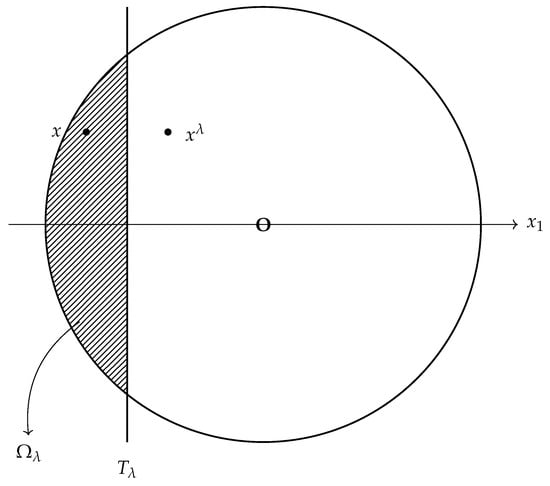
Figure 1. Moving planes on the unit ball.

For any given $\lambda \in \mathbb{R},$ let

$$\begin{array}{c}\hfill T_{\lambda }=\{x\in {\mathbb{R}}^n\mid x_1=\lambda \mathrm{for}\mathrm{some}\lambda \in \mathbb{R}\}\end{array}$$

be the moving planes,

$$\begin{array}{c}\hfill {\Sigma }_{\lambda }=\{x\in {\mathbb{R}}^n\mid x_1<\lambda \}\end{array}$$

be the region to the left of the plane, and

$$\begin{array}{c}\hfill x^{\lambda }=(2\lambda -x_1,x_2,...,x_n)\end{array}$$

be the reflection of x about the plane $T_{\lambda }.$

$$\begin{array}{c}\hfill \widetilde{{\Sigma }_{\lambda }}=\{x\mid x^{\lambda }\in {\Sigma }_{\lambda }\}\end{array}$$

is the reflection region of the plane, and

$$\begin{array}{c}\hfill {\Omega }_{\lambda }={\Sigma }_{\lambda }\cap B_1\left(0\right)\end{array}$$

is the intersection of $B_1\left(0\right)$ and ${\Sigma }_{\lambda }$.

Assume that $u(x,t)$ is a positive solution of Equation (5). We compare the values of $u(x,t)$ with

$$u_{\lambda }(x,t)=u(x^{\lambda },t),$$

and we denote

$$\begin{array}{c}\hfill w_{\lambda }(x,t)=u_{\lambda }(x,t)-u(x,t).\end{array}$$

The main part of the proof is to show that

$$\begin{array}{c}\hfill w_{\lambda }(x,t)\ge 0,(x,t)\in {\Omega }_{\lambda }\times \mathbb{R}.\end{array}$$

(6)

This provides a starting point to move the plane. Then, in the second step, we move the plane to the right as long as inequality (6) holds to its limiting position to show that u is symmetric about the limiting plane. A maximum principle is usually used to prove (6). Since $w_{\lambda }$ is an anti-symmetric function:

$$\begin{array}{c}\hfill w_{\lambda }(x,t)=-w_{\lambda }(x^{\lambda },t),\end{array}$$

for simplicity of notation, in the following, we denote $w_{\lambda }$ by w, ${\Sigma }_{\lambda }$ by $\Sigma$, and ${\Omega }_{\lambda }$ by $\Omega$. We first prove the following; Theorem 3 is referred to in [21].

Theorem 3.

(The maximum principle for the anti-symmetric functions on a parabolic cylinder) We add a time dimension on the unit ball with lower edge $t=\underline{t}$ and higher edge $t=T$; denote this thin cylinder as $\Omega \times (\underline{t},T]$ to be the narrow region in $\Sigma \times (\underline{t},T]$. Assume that $w(x,t)\in [C_{loc}^{1,1}(\Omega )\cap C\left(\overline{\Omega }\right)\cap {\mathcal{L}}_{2s}]\times C^1\left([\underline{t},T]\right)$ and is lower semi-continuous on $\overline{\Omega }\times (\underline{t},T]$. If

$$\begin{array}{c}\hfill \left\{\begin{array}{cc}{\displaystyle \frac{\partial w}{\partial t}}+{(-\Delta )}^{s}w=c(x,t)w(x,t),\hfill & in\Omega \times [\underline{t},T],\hfill \\ w(x,t)\ge 0,\hfill & in\Sigma \setminus \Omega \times [\underline{t},T],\hfill \\ w(x^{\lambda },t)=-w(x,t),\hfill & in\Sigma \times [\underline{t},T],\hfill \end{array}\right.\end{array}$$

(7)

where $c(x,t)$ is bounded from below in $\Omega \times [\underline{t},T]$; denote

$$\begin{array}{c}\hfill d\le width(\Omega ),\end{array}$$

then

$$\begin{array}{c}\hfill w(x,t)\ge min\{0,\underset{\Omega \times [\underline{t},T]}{inf}w(x,\underline{t})\}.\end{array}$$

(8)

In Section 3, we present proofs of Theorem 1. In Section 4, we present proofs of Theorem 3. In Section 5, we present proofs of Theorem 2, and therefore we obtain the radial symmetry and monotonicity of solutions of fractional parabolic equations. We hold a strong conviction that the ideas and methods presented here can be readily employed to investigate diverse nonlocal problems that involve more comprehensive operators and nonlinearities. Notice in Section 3, $\lambda$ is used to denote eigenvalues; in the Section 4 and Section 5, $\lambda$ is used to denote the reflection variable.

3. Proof of Theorem 1

Lemma 1.

The nonlocal fractional Laplacian operator defined by Equation (2) generates the semi-group in ${\mathbb{R}}_{+}^n\times \mathbb{R}$.

Proof. 

The resolvent for the fractional Laplacian ${(-▵)}^s$ is

$$\begin{array}{c}\hfill {({(-▵)}^s-z)}^{-1}f\left(x\right)={\displaystyle \frac{1}{{\left(2\pi \right)}^d}}{\int }_{{\mathbb{R}}^d}{e}^{ix·\xi }{\left(\right|\xi |}^{2s}{-z)}^{-1}\overline{f}\left(\xi \right)d\xi \end{array}$$

(9)

The poles of (9) are

$$\begin{array}{c}\hfill \xi =\pm (z^{{\displaystyle \frac{1}{2s}}})e^{i\theta },\theta \in [0,2\pi )\end{array}$$

Since $\xi$ is the integration variable and the integral is taken over all $\xi \in {\mathbb{R}}^d$, the poles are actually the values of z in the complex plane, such that there exists some $\xi$ such that ${\left|\xi \right|}^{2s}=z$. These values correspond to the positive real part of the complex plane, where $z=k$ with $k>0$. The set $\left\{\right|\xi {|}^{2s}:\xi \in {\mathbb{R}}^d\}$ is dense in $[0,\infty )$; for any $z>0$, we can find a $\xi \in {\mathbb{R}}^d$ such that ${\left|\xi \right|}^{2s}$ is arbitrarily close to z. Therefore, the fractional Laplacian operator ${(-▵)}^s$ generates the semi-group in ${\mathbb{R}}_{+}^n\times \mathbb{R}$. □

Lemma 2.

The nonlocal fractional Laplacian operator defined by Equation (2) is a self-adjoint and dense operator.

Proof. 

Consider the fractional Laplacian operator ${(-\Delta )}^s$ defined on an appropriate function space H; we will show that for all $u,v\in H$, we have

$$\begin{array}{c}\hfill <{(-\Delta )}^{s}u,v{>}_H=<u,{(-\Delta )}^{s}v{>}_H\end{array}$$

Let

$$\begin{array}{c}\hfill {(-\Delta )}^{s}u(\xi ,t)={\left|\xi \right|}^{2s}\widehat{u}(\xi ,t),\end{array}$$

be a Fourier transform representation of the fractional Laplacian applied to ${(-\Delta )}^{s}u(x,t)$, where

$$\begin{array}{c}\hfill {(-\Delta )}^{s}u(\xi ,t)={\int }_{{\mathbb{R}}^n}u(x,t)e^{-i\xi ·x}dx,\end{array}$$

the fractional Laplacian can be represented in Fourier space as

$$\begin{array}{c}\hfill F_x\left\{{(-\Delta )}^{s}u(x,t)\right\}(\xi ,t)={\left|\xi \right|}^{2s}u(x,t)\end{array}$$

where $F\{·\}$ denotes the Fourier transform.

Consider the inner product $<{(-\Delta )}^{s}u,v{>}_H$. Using Parseval’s identity, we have

$$\begin{array}{ccc}& & <{(-\Delta )}^{s}u,v{>}_H\hfill \\ & =& {\int }_{{\mathbb{R}}^n}{(-\Delta )}^{s}u(x,t)\overline{v(x,t)}dx\hfill \\ & =& {\int }_{{\mathbb{R}}^n}{F}_x^{-1}{\left\{\right|\xi |}^{2s}{F}_x\left\{u\right\}(\xi ,t)\}(x,t)\overline{F_x^{-1}\left\{F_x\left\{v\right\}(\xi ,t)\right\}(x,t)}dx\hfill \\ & =& {\int }_{{\mathbb{R}}^n}{\left|\xi \right|}^{2s}{F}_x\left\{u\right\}(\xi ,t)\overline{F_x\left\{v\right\}(\xi ,t)}d\xi (\mathrm{by}\mathrm{Parseval}’\mathrm{s}\mathrm{identity})\hfill \\ & =& {\int }_{{\mathbb{R}}^n}{F}_x\left\{u\right\}(\xi ,t)\overline{{\left|\xi \right|}^{2s}{F}_x\left\{v\right\}(\xi ,t)}d\xi \hfill \\ & =& {\int }_{{\mathbb{R}}^n}u\left(x\right)\overline{F_x^{-1}{\left\{\right|\xi |}^{2s}{F}_x\left\{v\right\}(\xi ,t)\}(x,t)}dx(\mathrm{by}\mathrm{Parseval}’\mathrm{s}\mathrm{identity}\mathrm{again})\hfill \\ & =& <u,{(-\Delta )}^{s}v{>}_H\hfill \end{array}$$

Since $<{(-\Delta )}^{s}u,v{>}_H=<u,{(-\Delta )}^{s}v{>}_H$ for all $u,v\in H$, we conclude that ${(-\Delta )}^s$ is a self-adjoint operator; therefore, the nonlocal fractional Laplacian operator is also a self-adjoint operator.

The domain of the fractional Laplacian ${(-\Delta )}^s$, which is ${\mathbb{R}}^n$, typically includes functions that are smooth or at least have some regularity properties, belonging to a Sobolev space $H^s\left({\mathbb{R}}^n\right)$. In ${\mathbb{R}}^n$, smooth functions $f\in C^{\infty }\left({\mathbb{R}}^n\right)$ are dense in various function spaces, including Sobolev spaces $H^s\left({\mathbb{R}}^n\right)$; this means that for any $u\in H^s\left({\mathbb{R}}^n\right)$, there exists a sequence $\left\{u_n\right\}\subset C^{\infty }\left({\mathbb{R}}^n\right)$ such that $u_n\to u$ in the $H^s$ norm. Since $C^{\infty }\left({\mathbb{R}}^n\right)$ is a subset of $H^s\left({\mathbb{R}}^n\right)$ and is dense therein, and the fractional Laplacian is well defined on $H^s\left({\mathbb{R}}^n\right)$, we can apply ${(-\Delta )}^s$ to each $u_n$ in the sequence; the resulting sequence $\left\{{(-\Delta )}^s{u}_n\right\}$ converges to $\left\{{(-\Delta )}^{s}u\right\}$ as $n\to \infty$. Therefore, the domain of the fractional Laplacian is dense in $H^s\left({\mathbb{R}}^n\right)$. □

Now, we will prove Theorem 1. First of all, we show the $L_p$-$L_q$ maximal regularity of solutions to the model problems in the whole space according to reference [20]:

$$\begin{array}{c}\hfill u_t+\Delta u=fin{\mathbb{R}}^n\times {\mathbb{R}}_{+}.\end{array}$$

(10)

Let $1<p,q<\infty$; we would like to show that the solution of (10) satisfies the $L_p$-$L_q$ maximal regularity estimate:

$$\begin{array}{c}\hfill \parallel e^{-\gamma t}{u}_t{\parallel }_{L_p(\mathbb{R},L_q\left({\mathbb{R}}^n\right)}+\parallel e^{-\gamma t}{\nabla }^2{u\parallel }_{L_p(\mathbb{R},L_q\left({\mathbb{R}}^n\right)}\le C{\parallel e^{-\gamma t}f\parallel }_{L_p(\mathbb{R},L_q\left({\mathbb{R}}^n\right))}\end{array}$$

(11)

for any $\gamma \ge 0$. We may assume that $f\in C_0^{\infty }({\mathbb{R}}^n\times {\mathbb{R}}_{+})$, because $C_0^{\infty }({\mathbb{R}}^n\times {\mathbb{R}}_{+})$ is dense in $L_{p,0}({\mathbb{R}}_{+},L_q\left({\mathbb{R}}^n\right))$.

To obtain the solution formula of (10), we first consider the resolvent problem corresponding to (10):

$$\begin{array}{c}\hfill \lambda u+u^{″}=f,\end{array}$$

(12)

apply the Laplace transform, we have

$$\begin{array}{c}\hfill \lambda U-{\xi }^{2}U=F,\end{array}$$

solving for U, we have

$$\begin{array}{c}\hfill U\left(\xi \right)={\displaystyle \frac{F\left(\xi \right)}{\lambda -{\xi }^2}}\end{array}$$

To obtain the exact formula of solutions of (10), we consider the equivalent homogeneous equation:

$$\begin{array}{c}\hfill {\displaystyle \frac{\partial u}{\partial t}}=-{\displaystyle \frac{{\partial }^{2}u}{\partial x^2}},\end{array}$$

(13)

Apply the Fourier transform to the problem related to x; we have

$$\begin{array}{c}\hfill {\displaystyle \frac{\partial \widehat{u}}{\partial t}}={\xi }^2\widehat{u}(\xi ,t),\end{array}$$

(14)

where

$$\begin{array}{c}\hfill \widehat{u}(\xi ,t)={\displaystyle \frac{1}{\sqrt{2\pi }}}{\int }_{-\infty }^{\infty }{e}^{-ix\xi }u(x,t)dx,\end{array}$$

(15)

combine (14) and (15); we have

$$\begin{array}{c}\hfill {\displaystyle \frac{\partial \widehat{u}}{\partial t}}={\xi }^2{\displaystyle \frac{1}{\sqrt{2\pi }}}{\int }_{-\infty }^{\infty }{e}^{-ix\xi }u(x,t)dx.\end{array}$$

(16)

Solve (14); we have

$$\begin{array}{c}\hfill \widehat{u}(\xi ,t)=C_0{e}^{{\xi }^{2}t}\end{array}$$

(17)

where $C_0=\widehat{u}(\xi ,0)$ is the initial value, and take ${\xi }^2=\lambda$ as the eigenvalues so that (17) generates a semi-group.

Therefore, we obtain the solution formula of (10):

$$\begin{array}{c}\hfill u(x,t)={\mathcal{L}}^{-1}[{\displaystyle \frac{\mathcal{L}\left[f\right](\xi ,\lambda )}{\lambda -{\left|\xi \right|}^2}}](x,t),\end{array}$$

(18)

where $\mathcal{L}$ and ${\mathcal{L}}^{-1}$ denote the Fourier–Laplace transform and its inverse, defined by

$$\begin{array}{c}\hfill \left[\mathcal{L}f\right](\xi ,\lambda )=\int {\int }_{{\mathbb{R}}^{n+1}}{e}^{-\lambda t-ix·\xi }f(x,t)dxdt=\mathcal{F}\left[e^{-\lambda t}f\right](\xi ,\tau ),\end{array}$$

$$\begin{array}{ccc}\hfill \left[{\mathcal{L}}^{-1}g\right](x,t)& =& {\displaystyle \frac{1}{{\left(2\pi \right)}^{n+1}}}\int {\int }_{{\mathbb{R}}^{n+1}}{e}^{\lambda t+ix·\xi }g(\xi ,\lambda )d\xi d\tau \hfill \\ & =& e^{\lambda t}{\mathcal{F}}^{-1}\left[g(\xi ,\lambda +i\tau )\right](x,t),\lambda =\gamma +i\tau ,\hfill \end{array}$$

respectively. In particular, $u_t$ is given by the formula:

$$\begin{array}{c}\hfill u_t(x,t)={\mathcal{L}}^{-1}[{\displaystyle \frac{\lambda \mathcal{L}\left[f\right](\xi ,\lambda )}{\lambda -{\left|\xi \right|}^2}}](x,t).\end{array}$$

Set

$$\begin{array}{c}\hfill k_{\gamma }(\tau ,x)={\mathcal{F}}^{-1}\left[\lambda \right(\lambda -{\left|\xi \right|}^2{)}^{-1}]\left(x\right),\lambda =\gamma +i\tau ,\end{array}$$

$$\begin{array}{c}\hfill \left[K_{\gamma }g\right]\left(x\right)={\int }_{{\mathbb{R}}^n}{k}_{\gamma }(\tau ,x-y)g\left(y\right)dy.\end{array}$$

Then, we have

$$\begin{array}{c}\hfill e^{-\gamma t}{u}_t={\mathcal{F}}_{\tau }^{-1}\left[K_{\gamma }\left(\tau \right){\mathcal{F}}_t\left[e^{-\gamma t}f\right]\left(t\right)\right].\end{array}$$

(19)

Employing the same arguments and process in [20], only different in the denominator in the solution formula (26), by the $\mathcal{R}$-boundedness of the families $\{K_{\gamma }\left(\tau \right)\mid \tau \in \mathbb{R}\left\{0\right\}\}$ and $\{\tau {\partial }_{\tau }{K}_{\gamma }\left(\tau \right)\mid \tau \in \mathbb{R}\left\{0\right\}\}$, we obtain

$$\begin{array}{c}\hfill \parallel e^{-\gamma t}{u}_t{\parallel }_{L_p(\mathbb{R},L_q\left({\mathbb{R}}^n\right))}\le C{\parallel e^{-\gamma t}f\parallel }_{L_p(\mathbb{R},L_q\left({\mathbb{R}}^n\right))},\forall \gamma \ge 0.\end{array}$$

(20)

We can also see that in [20]:

$$\begin{array}{c}\hfill \parallel e^{-\gamma t}{\nabla }^2{u\parallel }_{L_p(\mathbb{R},L_q\left({\mathbb{R}}^n\right))}\le C{\parallel e^{-\gamma t}f\parallel }_{L_p(\mathbb{R},L_q\left({\mathbb{R}}^n\right))},\forall \gamma \ge 0.\end{array}$$

(21)

Combining (20) with (21), we obtain (11).

Since we have proved the maximal $L_p$-$L_q$ regularity of the model equation (10), to apply the result on proving the maximal $L_p$-$L_q$ regularity of the nonlocal parabolic fractional Laplacian equations (1), use the following procedure, since

$$\begin{array}{c}\hfill {(-\Delta )}^{s}u(\xi ,t)={\left|\xi \right|}^{2s}\widehat{u}(\xi ,t),\end{array}$$

where $\widehat{u}=\mathcal{F}\left(u\right)$ is the Fourier transform of u, i.e.,

$$\begin{array}{c}\hfill \mathcal{F}\left(u\right)\left(\xi \right)={\int }_{{\mathbb{R}}^n}{e}^{-2\pi ix·\xi }u(x,t)dx.\end{array}$$

The Fourier transform of homogeneous equation

$$\begin{array}{c}\hfill {\displaystyle \frac{\partial u}{\partial t}}(x,t)+{(-\Delta )}^{s}u(x,t)=0\end{array}$$

is

$$\begin{array}{c}\hfill {\displaystyle \frac{\partial \widehat{u}}{\partial t}}(\xi ,t)=-{\left|\xi \right|}^{2s}\widehat{u}(\xi ,t),\end{array}$$

(22)

we derive

$$\begin{array}{c}\hfill \widehat{u}(\xi ,t)=C_0{e}^{-{\left|\xi \right|}^{2s}t}\end{array}$$

(23)

for some constant $C_0=\widehat{u}(\xi ,0)$, and take $-{\left|\xi \right|}^{2s}=\lambda$ as the eigenvalues so that (23) generates a semi-group. Therefore, the above process of finding the maximal regularity of the model problem could be applied to the nonlocal parabolic fractional Laplacian equations.

In this paper, we consider the case where the boundary condition is zero, in which $u{\mid }_{\partial B_1\left(0\right)}=0$. Therefore, the maximal regularity of nonlocal parabolic fractional Laplacian equations in the whole space can be applied to our problem, which proves the Theorem 1.

In [18], the author briefly elucidates the underlying logic and principles governing the existence of maximal regularity for parabolic and hyperbolic differential equations. Based on this reference, we can verify that the prerequisite for the existence of maximal regularity for parabolic differential equations is that the eigenvalues of the operator related to spatial variables must be less than 1. In (11), we observe that as $\gamma \to \infty$ and $t>0$, $\parallel e^{-\gamma t}{\nabla }^2{u\parallel }_{L_p(\mathbb{R},L_q\left({\mathbb{R}}^n\right)}$ could be bounded by 1; however, when $\gamma$ is not sufficiently large or $t<0$, to ensure that the eigenvalues of the nonlocal fractional Laplacian operator remain less than 1, we impose the condition $u(x,t)\stackrel{a.e.}{\to }{u}_0(x,t)$ for $(x,t)\in B_1\left(0\right)\times \mathbb{R}$ in Theorem 2, where we take the measure space $(X,\Sigma ,\mu )$ as the following:

$$\begin{array}{c}\hfill X={\mathbb{R}}^n\cap B_1\left(0\right)\end{array}$$

$$\begin{array}{c}\hfill E=\pm (z^{{\displaystyle \frac{1}{2s}}}),z>0,z={\left|\xi \right|}^{2s},\xi \in {\displaystyle \frac{p}{q}}\mathrm{where}p,q\in \mathbb{Z},p,q\ne 0,\end{array}$$

therefore, we have $u_n(x,t)\to u_0(x,t)$ for all $x\in X\setminus E$ to control the growth of ${(-\Delta )}^{s}u(x,t)$ on those uncountable sets where the eigenvalues of ${(-\Delta )}^{s}u(x,t)$ could be defined, by the definition of fractional Laplacian operator, since we take the integration variable $y\in {\mathbb{R}}^n$, the eigenvalue of ${(-▵)}^{s}u(x,t)$ could be controlled less than 1.

4. Proof of Theorem 3

In this section, we will provide the detailed proof of Theorem 3 for the fractional parabolic equations. Using Theorem 3 (the maximum principle), we also give the detailed proof of Theorem 2 in the next section.

If (8) does not hold, then the lower semi-continuity of $w(x,t)$ on $\overline{\Omega }\times [\underline{t},T]$ guarantees that there exists an $(x^o,t^o)\in \Omega \times [\underline{t},T]$ such that

$$\begin{array}{c}\hfill w(x^o,t^o)=\underset{\Omega \times (\underline{t},T]}{min}w<0.\end{array}$$

Since $(x^o,t^o)$ is the minimum point, thus

$$\begin{array}{c}\hfill {\displaystyle \frac{\partial w(x^o,t^o)}{\partial t}}=0,\end{array}$$

(24)

and one can further deduce from condition (7) that $(x^o,t^o)$ is in the interior of $\Omega \times [\underline{t},T]$. We have

$$\begin{array}{ccc}\hfill & & {(-\Delta )}^{s}w(x^o,t^o)\hfill \\ & =& C_{n,s}P.V.{\int }_{{\mathbb{R}}^n}{\displaystyle \frac{w(x^o,t^o)-w(y,t^o)}{|x^o{-y|}^{n+2s}}}dy\hfill \\ & =& C_{n,s}P.V.\left\{{\int }_{\Sigma }{\displaystyle \frac{w(x^o,t^o)-w(y,t^o)}{|x^o{-y|}^{n+2s}}}dy+{\int }_{\tilde{\Sigma }}{\displaystyle \frac{w(x^o,t^o)-w(y,t^o)}{|x^o{-y|}^{n+2s}}}dy\right\}\hfill \\ & =& C_{n,s}P.V.\left\{{\int }_{\Sigma }{\displaystyle \frac{w(x^o,t^o)-w(y,t^o)}{|x^o{-y|}^{n+2s}}}dy+{\int }_{\Sigma }{\displaystyle \frac{w(x^o,t^o)-w(y^{\lambda },t^o)}{|x^o-y^{\lambda }{|}^{n+2s}}}dy\right\}\hfill \\ & =& C_{n,s}P.V.\left\{{\int }_{\Sigma }{\displaystyle \frac{w(x^o,t^o)-w(y,t^o)}{|x^o{-y|}^{n+2s}}}dy+{\int }_{\Sigma }{\displaystyle \frac{w(x^o,t^o)+w(y,t^o)}{|x^o-y^{\lambda }{|}^{n+2s}}}dy\right\}\hfill \\ & \le & C_{n,s}\left\{{\int }_{\Sigma }{\displaystyle \frac{w(x^o,t^o)-w(y,t^o)}{|x^o-y^{\lambda }{|}^{n+2s}}}dy+{\displaystyle \frac{w(x^o,t^o)+w(y,t^o)}{|x^o-y^{\lambda }{|}^{n+2s}}}dy\right\}\hfill \\ & =& C_{n,s}{\int }_{\Sigma }{\displaystyle \frac{2w(x^o,t^o)}{|x^o-y^{\lambda }{|}^{n+2s}}}.\hfill \end{array}$$

(25)

Choose a ball centered at $(x^o,t^o)\in \Sigma \times [\underline{t},T]$ with radius $2l$, and let $D=B_{2l}(x^o,t^o)\cap \tilde{\Sigma }$, see Figure 2. Then,

$$\begin{array}{ccc}\hfill & & {\int }_{\Sigma }{\displaystyle \frac{1}{|x^o-y^{\lambda }|}}dy\ge {\int }_D{\displaystyle \frac{1}{|x^o{-y|}^{n+2s}}}dy\hfill \\ & \ge & vol\left(D\right)·{\displaystyle \frac{1}{{\left(2d\right)}^{n+2s}}}\ge c{\left(2d\right)}^n·{\displaystyle \frac{1}{{\left(2d\right)}^{n+2s}}}={\displaystyle \frac{c}{d^{2s}}}.\hfill \end{array}$$

(26)

Combining (7), (24), (25), and (26), we deduce

$$\begin{array}{ccc}& & {(-\Delta )}^{s}w(x^o,t^o)=c(x^o,t^o)w(x^o,t^o)\hfill \\ & \le & C_{n,s}{\int }_{\Sigma }{\displaystyle \frac{2w(x^o,t^o)}{|x^o-y^{\lambda }{|}^{n+2s}}}\hfill \\ & \le & {\displaystyle \frac{cw(x^o,t^o)}{d^{2s}}},\hfill \end{array}$$

then, we derive

$$\begin{array}{c}\hfill {\displaystyle \frac{c}{d^{2s}}}\le c(x^o,t^o),\end{array}$$

since $\Omega \times (\underline{t},T]$ is a narrow region, d would be sufficiently small; since c is bounded, we derive a contradiction. Therefore, (8) must be valid.

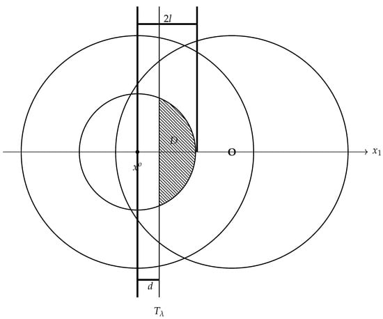
Figure 2. The region of $D=B_{2l}\cap \widetilde{{\Sigma }_{\lambda }}$.

So far, we have proved the Theorem 3.

5. Proof of Theorem 2

Step 1: Begin moving the plane from near the left end of $B_1\left(0\right)$ along the $x_1$ axis, but do not reach origin,

so then

$$\begin{array}{c}\hfill |x^{\lambda }|<|x|,\end{array}$$

we derive

$$\begin{array}{c}\hfill f(t,|x^{\lambda }|,u_{\lambda })-f(t,\left|x\right|,u_{\lambda })\ge 0.\end{array}$$

We deduce from the Equation (5) and $\left(f1\right)$, $\left(f2\right)$ that $w_{\lambda }$ satisfies

$$\begin{array}{ccc}\hfill & & {\displaystyle \frac{\partial w_{\lambda }}{\partial t}}(x,t)+{(-\Delta )}^s{w}_{\lambda }(x,t)\hfill \\ & =& f(t,|x^{\lambda }|,u_{\lambda })-f(t,\left|x\right|,u)\hfill \\ & =& f(t,|x^{\lambda }|,u_{\lambda })-f(t,\left|x\right|,u_{\lambda })+f(t,\left|x\right|,u_{\lambda })-f(t,\left|x\right|,u)\hfill \\ & \ge & f(t,|x|,u_{\lambda })-f(t,\left|x\right|,u)\hfill \\ & =& {\displaystyle \frac{f(t,|x|,u_{\lambda })-f(t,\left|x\right|,u)}{u_{\lambda }(x,t)-u(x,t)}}{w}_{\lambda }(x,t)\hfill \\ & :=& c_{\lambda }(x,t)w_{\lambda }(x,t),\hfill \end{array}$$

(27)

where $c_{\lambda }(x,t)={\displaystyle \frac{f(t,|x|,u_{\lambda })-f(t,\left|x\right|,u)}{u_{\lambda }(x,t)-u(x,t)}}$ is bounded.

We first prove that for $\lambda$ sufficiently close to $-1$, we have:

$$\begin{array}{c}\hfill w_{\lambda }(x,t)\ge 0.\end{array}$$

(28)

Let $w_{\lambda }$ be w in Theorem 3, we have

$$\begin{array}{c}\hfill {\displaystyle \frac{\partial w_{\lambda }}{\partial t}}+{(-\Delta )}^s{w}_{\lambda }=c(x,t)w_{\lambda }(x,t),(x,t)\in {\Omega }_{\lambda }\times [\underline{t},T],\end{array}$$

according to Theorem 3, we conclude that for $\lambda$ sufficiently close to $-1$ when ${\Omega }_{\lambda }$ is narrow,

$$\begin{array}{c}\hfill w_{\lambda }(x,t)\ge min\{0,\underset{{\Omega }_{\lambda }\times [\underline{t},T]}{inf}{w}_{\lambda }(x,\underline{t})\},w_{\lambda }\in [C_{loc}^{1,1}\left({\Omega }_{\lambda }\right)\cap C\left(\overline{{\Omega }_{\lambda }}\right)\cap {\mathcal{L}}_{2s}]\times C^1\left([\underline{t},T]\right).\end{array}$$

Let

$$\begin{array}{c}\hfill \overline{w}=e^{m(t-\underline{t})}{w}_{\lambda }(x,t),m>0,\end{array}$$

from (27), we derive

$$\begin{array}{c}\hfill {\displaystyle \frac{\partial \overline{w}}{\partial t}}+{(-▵)}^s\overline{w}\ge \overline{c}\overline{w},\end{array}$$

(29)

with $\overline{c}$ is still bounded.

Suppose otherwise that (28) does not hold, then $\overline{w}(x,t)$ is negative somewhere; hence, there exists an $x^o\in {\Omega }_{\lambda }$ and $t^o\in [\underline{t},T]$ such that

$$\begin{array}{c}\hfill \overline{w}(x^o,t^o)=\underset{{\Omega }_{\lambda }\times (\underline{t},T]}{min}\overline{w}<0.\end{array}$$

If $t^o<T$, ${\displaystyle \frac{\partial \overline{w}}{\partial t}}(x^o,t^o)=0$. If $t^o=T$, ${\displaystyle \frac{\partial \overline{w}}{\partial t}}(x^o,t^o)\le 0.$ Combine with (29), we derive

$$\begin{array}{c}\hfill {(-\Delta )}^s\overline{w}(x^o,t^o)\ge \overline{c}(x^o,t^o)\overline{w}(x^o,t^o),\end{array}$$

from (26), we also have

$$\begin{array}{c}\hfill {(-\Delta )}^s\overline{w}(x^o,t^o)\le {\displaystyle \frac{c}{d^{2s}}}\overline{w}(x^o,t^o),\end{array}$$

(30)

where $d\le width\left({\Omega }_{\lambda }\right)$; then, we derive

$$\begin{array}{c}\hfill {\displaystyle \frac{c}{d^{2s}}}\le \overline{c}(x^o,t^o),\end{array}$$

which is a contradiction for d sufficiently small. Thus,

$$\begin{array}{c}\hfill \overline{w}(x,t)\ge min\{0,\underset{x\in {\Omega }_{\lambda }}{inf}\overline{w}(x,\underline{t})\},\forall (x,t)\in {\Omega }_{\lambda }\times (\underline{t},T),\end{array}$$

$$\begin{array}{c}\hfill e^{m(t-\underline{t})}{w}_{\lambda }(x,t)\ge min\{0,\underset{x\in {\Omega }_{\lambda }}{inf}{w}_{\lambda }(x,\underline{t})\},\end{array}$$

$$\begin{array}{c}\hfill w_{\lambda }(x,t)\ge e^{-m(t-\underline{t})}min\{0,\underset{x\in {\Omega }_{\lambda }}{inf}{w}_{\lambda }(x,\underline{t})\}.\end{array}$$

$w_{\lambda }(x,t)$ is bounded from below. Let $\underline{t}\to -\infty$, $w_{\lambda }(x,t)\to \ge 0$.

Therefore, (28) is proved if ${\Omega }_{\lambda }$ is narrow.

Step 2: The inequality (28) provides a starting point, from which we can carry out the moving. Now, we move the plane continuously to the right until its limiting position, as long as (28) holds.

Define

$$\begin{array}{c}\hfill {\lambda }_0=sup\{\lambda \le 0\mid w_{\mu }(x,t)\ge 0,\forall (x,t)\in {\Omega }_{\mu }\times \mathbb{R},\mu \le \lambda \},\end{array}$$

we will prove ${\lambda }_0=0$.

Otherwise, if ${\lambda }_0<0$, we will show that $T_{{\lambda }_0}$ can be moved further to the right and we will have

$$\begin{array}{c}\hfill w_{\lambda }(x,t)\ge 0,(x,t)\in {\Sigma }_{{\lambda }_0}\times \mathbb{R},\forall {\lambda }_0<\lambda \le {\lambda }_0+ϵ.\end{array}$$

Suppose ${\lambda }_0<0$; we want to first show

$$\begin{array}{c}\hfill w_{{\lambda }_0}(x,t)>0,(x,t)\in {\Omega }_{{\lambda }_0}\times \mathbb{R}.\end{array}$$

(31)

Suppose otherwise, (31) does not hold, then there exists $(x^o,t^o)\in {\Omega }_{{\lambda }_0}\times \mathbb{R}$ such that $w_{{\lambda }_0}(x^o,t^o)=0$. Since $w_{{\lambda }_0}(x,t)\ge 0$ inside ${\Omega }_{{\lambda }_0}\times \mathbb{R}$ as step 1 has proved, $(x^o,t^o)$ is the minimum point, thus ${\displaystyle \frac{\partial w_{{\lambda }_0}}{\partial t}}(x^o,t^o)=0$; following from (27), we derive

$$\begin{array}{c}\hfill {\displaystyle \frac{\partial w_{{\lambda }_0}}{\partial t}}(x^o,t^o)+{(-\Delta )}^s{w}_{{\lambda }_0}(x^o,t^o)\ge c_{{\lambda }_0}(x^o,t^o)w_{{\lambda }_0}(x^o,t^o),\end{array}$$

so that

$$\begin{array}{c}\hfill {(-▵)}^s{w}_{{\lambda }_0}(x^o,t^o)\ge 0.\end{array}$$

It follows that

$$\begin{array}{ccc}\hfill & & 0\le {(-\Delta )}^s{w}_{{\lambda }_0}(x^o,t^o)\hfill \\ & =& C_{n,s}P.V.{\int }_{{\mathbb{R}}^n}{\displaystyle \frac{-w_{{\lambda }_0}(y,t^o)}{|x^o{-y|}^{n+2s}}}dy\hfill \\ & =& C_{n,s}P.V.\left\{{\int }_{{\Sigma }_{{\lambda }_0}}{\displaystyle \frac{-w_{{\lambda }_0}(y,t^o)}{|x^o{-y|}^{n+2s}}}dy+{\int }_{\widetilde{{\Sigma }_{{\lambda }_0}}}{\displaystyle \frac{-w_{{\lambda }_0}(y,t^o)}{|x^o{-y|}^{n+2s}}}dy\right\}\hfill \\ & =& C_{n,s}P.V.\left\{{\int }_{{\Sigma }_{{\lambda }_0}}{\displaystyle \frac{-w_{{\lambda }_0}(y,t^o)}{|x^o{-y|}^{n+2s}}}dy+{\int }_{{\Sigma }_{{\lambda }_0}}{\displaystyle \frac{-w_{{\lambda }_0}(y^{{\lambda }_0},t^o)}{|x^o-y^{{\lambda }_0}{|}^{n+2s}}}dy\right\}\hfill \\ & =& C_{n,s}P.V.\left\{{\int }_{{\Sigma }_{{\lambda }_0}}{\displaystyle \frac{-w_{{\lambda }_0}(y,t^o)}{|x^o{-y|}^{n+2s}}}dy+{\int }_{{\Sigma }_{{\lambda }_0}}{\displaystyle \frac{w_{{\lambda }_0}(y,t^o)}{|x^o-y^{{\lambda }_0}{|}^{n+2s}}}dy\right\}\hfill \\ & =& C_{n,s}P.V.{\int }_{{\Sigma }_{{\lambda }_0}}{w}_{{\lambda }_0}(y,t^o)\left\{{\displaystyle \frac{1}{|x^o-y^{{\lambda }_0}{|}^{n+2s}}}-{\displaystyle \frac{1}{|x^o{-y|}^{n+2s}}}\right\}dy\hfill \\ & \le & 0,\hfill \end{array}$$

(32)

since

$$\begin{array}{c}\hfill {\displaystyle \frac{1}{|x^o-y^{{\lambda }_0}{|}^{n+2s}}}-{\displaystyle \frac{1}{|x^o{-y|}^{n+2s}}}<0,\end{array}$$

this implies that

$$w_{{\lambda }_0}(y,t^o)\equiv 0,in{\Omega }_{{\lambda }_0}\times \mathbb{R},$$

(33)

we derive a contradiction, since the plane $T_{{\lambda }_0}$ did not reach the origin. If we take a point $\overline{x}$ on the curved part $\partial {\Omega }_{{\lambda }_0}$, then its reflection point ${\overline{x}}^{{\lambda }_0}$ is in the interior of the ball, $u({\overline{x}}^{{\lambda }_0},t)>0$, $w_{{\lambda }_0}(\overline{x},t)=u({\overline{x}}^{{\lambda }_0},t)-u(\overline{x},t)>0$, which contradicts (33). Therefore, (31) is proved.

However, since for all $x\in X\setminus E$, $u_n(x,t)\to u(x,t)$, we proceed to establish $w_{{\lambda }_0}(x,t)$ is bounded away from 0:

$$\begin{array}{c}\hfill inf{w}_{{\lambda }_0}(x,t)>c_o>0,(x,t)\in {\Omega }_{{\lambda }_0-\delta }\times \mathbb{R}.\end{array}$$

(34)

Suppose (34) is violated, then there exists $(x_k,t_k)\in {\Omega }_{{\lambda }_0-\delta }\times \mathbb{R}$ such that $w_{{\lambda }_0}(x_k,t_k)\to 0$. Without loss of generality, by the Bolzano–Weierstrass theorem, there exist some subsequences of $x_k$ (here, we still denote this subsequence by $x_k$ for convenience) such that $x_k\to x^o$ in ${\Omega }_{{\lambda }_0-\delta }$.

Let

$$\begin{array}{c}\hfill w_k(x,t)=w_{{\lambda }_0}(x,t+t_k),c_k(x,t)=c_{{\lambda }_0}(x,t+t_k),\end{array}$$

We rewrite Lemma 3.1 from [22] as the following, as we will use it later:

Lemma 3.

Let $s\in (0,1)$, and let ${\left(L_k\right)}_{k\in \mathbb{N}}$ be a sequence of nonlocal fractional Laplacian operators. Let ${\left(u_k\right)}_{k\in \mathbb{N}}$ and ${\left(f_k\right)}_{k\in \mathbb{N}}$ be sequences of functions satisfying in the weak sense

$$\begin{array}{c}\hfill {\partial }_t{u}_k-L_k{u}_k=f_{k}inI\times K\end{array}$$

(35)

for a given bounded interval $I\subset (-\infty ,0]$ and a bounded domain $K\subset {\mathbb{R}}^n$. Assume that $L_k$ have spectral measures ${\mu }_k$ converging to a spectral measure μ. Let L be the operator associated with μ (weak limit of $L_k$), and suppose that, for some functions, u and f, the following hypotheses hold:

1. 

$u_k\to u$ uniformly in compact sets of $(-\infty ,0]\times {\mathbb{R}}^n$

2. 

$f_k\to f$ uniformly in $I\times K$,

3. 

${sup}_{t\in I}|u_k{(t,x)|\le C(1+\left|x\right|}^{2s-ϵ})$ for some $ϵ>0$, and for all $x\in {\mathbb{R}}^n$.

Then, u satisfies

$$\begin{array}{c}\hfill {\partial }_{t}u-Lu=finI\times K\end{array}$$

(36)

in the weak sense.

By the assumption that $w_k(x_k,0)=w_{{\lambda }_0}(x_k,t_k)\to 0$ for some $(x_k,t_k)\in {\Omega }_{{\lambda }_0-\delta }\times \mathbb{R}$, and given that $w_k$ satisfies a certain compactness property, the compactness is derived from the Arzelà–Ascoli theorem, which guarantees that if $w_k$ is bounded in a suitable fractional Sobolev space, then it converges locally uniformly in $C^{\alpha }$ for $\alpha >0$. Therefore, $w_k(x_k,0)$ converges locally uniformly to $\overline{w}(x^o,0)$ and $\overline{w}(x^o,0)=0$. It follows that,

$$\begin{array}{c}\hfill {(-\Delta )}^s\overline{w}(x^o,0)=\overline{c}(x^o,0)\overline{w}(x^o,0)=0\end{array}$$

We also have

$$\begin{array}{c}\hfill {(-\Delta )}^s\overline{w}(x^o,0)=C_{n,s}PV{\int }_{{\mathbb{R}}^n}{\displaystyle \frac{-\overline{w}(y,0)}{|x^o{-y|}^{n+2s}}}dy\le 0\end{array}$$

which forces

$$\begin{array}{c}\hfill \overline{w}(y,0)\equiv 0,\forall y\in {\mathbb{R}}^n\end{array}$$

(37)

Let $u_k(x,t)=u(x,t+t_k)$; suppose there are some sequences $x_k\in X\setminus E$ such that $u_k(x_k,0)$ converges uniformly to $\overline{u}(x^o,0)$, and $f(0,u_k)$ converges uniformly to $\overline{f}(0,\overline{u})$.

By a Strong Maximum principle:

Lemma 4.

Assume that $\overline{u}(x,0)\in [C_{loc}^{1,1}\left({\Omega }_{\lambda }\right)\cap C\left(\overline{{\Omega }_{\lambda }}\right)\cap {\mathcal{L}}_{2s}]\times 0$ satisfies

$$\begin{array}{c}\hfill \left\{\begin{array}{cc}{\displaystyle \frac{\partial \overline{u}(x,0)}{\partial t}}+{(-\Delta )}^s\overline{u}(x,0)=\overline{f}(0,\overline{u}),\hfill & (x,0)\in {\Omega }_{\lambda }\times 0,\hfill \\ \overline{u}(x,0)\ge 0,\hfill & (x,0)\in {\Omega }_{\lambda }\times 0\hfill \end{array}\right.\end{array}$$

(38)

we have either

$$\begin{array}{c}\hfill \overline{u}(x,0)>0,x\in B_1\left(0\right),\end{array}$$

or

$$\begin{array}{c}\hfill \overline{u}(x,0)\equiv 0,x\in {\mathbb{R}}^n.\end{array}$$

If $\overline{u}(x^o,0)>0,x^o\in B_1\left(0\right)$, $\overline{w}(x^o,0)>0$ somewhere, but we already derive $\overline{w}(x^o,0)\equiv 0$ in (37), see Figure 3, then we must have $\overline{u}(x^o,0)\equiv 0$, $x^o\in {\mathbb{R}}^n$. Thus, $u_k(x_k,0)$ converges to 0 uniformly in ${\mathbb{R}}^n$. Until now, the hypotheses in Lemma 3 have been satisfied; then, we can guarantee the equation of the form

$$\begin{array}{c}\hfill {\displaystyle \frac{\partial w_k(x_k,0)}{\partial t}}+{(-\Delta )}^s{w}_k(x_k,0)=c_k(x_k,0)w_k(x_k,0)\end{array}$$

(39)

could converge to the form

$$\begin{array}{c}\hfill {\displaystyle \frac{\partial \overline{w}(x,0)}{\partial t}}+{(-\Delta )}^s\overline{w}(x,0)=\overline{c}(x,0)\overline{w}(x,0)\end{array}$$

(40)

in the weak sense. In the context of weak sense, the equation is understood in the distributional sense, meaning that the equation holds in the limit after multiplication by a test function and subsequent integration. For an arbitrary test function $\varphi \in C_c^{\infty }(I\times K)$, the following holds:

$$\begin{array}{c}\hfill {\int }_{I\times K}{w}_k({\partial }_t\varphi +L_k\varphi )dxdt={\int }_{I\times K}{c}_k\varphi dxdt,\end{array}$$

(41)

Furthermore, as the limit is taken, w fulfills the weak formulation

$$\begin{array}{c}\hfill {\int }_{I\times K}w({\partial }_t\varphi +L\varphi )dxdt={\int }_{I\times K}c\varphi dxdt,\end{array}$$

(42)

for all test functions $\varphi$, where $L_k$ in (41) and L in (42) are fractional Laplacian operators. We can also guarantee the equation of the form

$$\begin{array}{c}\hfill {\displaystyle \frac{\partial u_k(x_k,0)}{\partial t}}+{(-\Delta )}^s{u}_k(x_k,0)=f_k(0,u_k)\end{array}$$

(43)

could converge to the form

$$\begin{array}{c}\hfill {\displaystyle \frac{\partial \overline{u}(x,0)}{\partial t}}+{(-\Delta )}^s\overline{u}(x,0)=f(0,\overline{u})\end{array}$$

(44)

in the weak sense. For an arbitrary test function $\varphi \in C_c^{\infty }(I\times K)$, the following holds:

$$\begin{array}{c}\hfill {\int }_{I\times K}{u}_k({\partial }_t\varphi +L_k\varphi )dxdt={\int }_{I\times K}{f}_k\varphi dxdt,\end{array}$$

(45)

as the limit is taken, u fulfills the weak formulation

$$\begin{array}{c}\hfill {\int }_{I\times K}u({\partial }_t\varphi +L\varphi )dxdt={\int }_{I\times K}f\varphi dxdt.\end{array}$$

(46)

Notice that we use the Lemma 3 to verify the weak convergence; however, by regularity theory for parabolic equations in [22], it is easy to check that (39) converges to (40) uniformly and (43) converges to (44) uniformly. More content related to the regularity of fractional function could refer to [23].

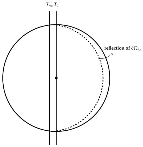
Figure 3. Reflection of the curved part of $\partial {\Omega }_{{\lambda }_0}$.

In order to derive a contradiction for large k in (41), let

$$\begin{array}{c}\hfill w_k(x_k,0)\equiv w_{{\lambda }_0}(x_k,t_k)=m_k,\end{array}$$

(47)

which converges to 0 uniformly.

Let

$$\begin{array}{c}\hfill v_k(x,t)=w_k(x,t)-2m_k\eta \left({ϵ}_k(t-t_k)\right),\end{array}$$

(48)

where $\eta \left(t\right)\in C_0^{\infty }$ is a cut-off function such that $|{\eta }^{\prime }\left(t\right)|\le c$ and

$$\begin{array}{c}\hfill \eta \left(t\right)=\left\{\begin{array}{cc}1,\hfill & \left|t\right|\le 1,\hfill \\ 0,\hfill & \left|t\right|\ge 2.\hfill \end{array}\right.\end{array}$$

$v_k(x,t)$ attains its minimum at some point, say $({\overline{x}}_k,{\overline{t}}_k)$ in ${\Omega }_{{\lambda }_0-\delta }\times (t_k-2,t_k+2)$; this implies

$$\begin{array}{c}\hfill {\displaystyle \frac{\partial v_k}{\partial t}}({\overline{x}}_k,{\overline{t}}_k)=0.\end{array}$$

(49)

Combining (48) and (49), it also implies

$$\begin{array}{c}\hfill {\displaystyle \frac{\partial v_k}{\partial t}}({\overline{x}}_k,{\overline{t}}_k)={\displaystyle \frac{\partial w_k}{\partial t}}({\overline{x}}_k,{\overline{t}}_k)-2m_k{ϵ}_k=0,\end{array}$$

and

$$\begin{array}{c}\hfill {\displaystyle \frac{\partial w_k}{\partial t}}({\overline{x}}_k,{\overline{t}}_k)\sim m_k{ϵ}_k,\end{array}$$

Combining (47) and (48), it is easy to deduce

$$\begin{array}{c}\hfill v_k(x_k,0)=w_k(x_k,0)-2m_k=m_k-2m_k=-m_k,\end{array}$$

thus

$$\begin{array}{c}\hfill v_k({\overline{x}}_k,{\overline{t}}_k)\le -m_k.\end{array}$$

Since we have

$$\begin{array}{c}\hfill {(-\Delta )}^s{v}_k({\overline{x}}_k,{\overline{t}}_k)\le {\displaystyle \frac{c}{{\left[d({\overline{x}}_k,T_{{\lambda }_0})\right]}^{2s}}}{v}_k({\overline{x}}_k,{\overline{t}}_k)\le -c_1{m}_k,\end{array}$$

(50)

where $c_1>0$, which is a contradiction. Hence, we have proved (34).

Since $w_{\lambda }$ depends on $\lambda$ continuously, there exists $ϵ>0$ and $ϵ<\delta$, such that for all $\lambda \in ({\lambda }_0,{\lambda }_0+ϵ)$, we have

$$\begin{array}{c}\hfill w_{\lambda }(x,t)\ge 0,(x,t)\in {\Omega }_{{\lambda }_0-\delta }\times \mathbb{R}.\end{array}$$

(51)

Now apply the Maximum principle 3 and, in our case, the narrow region is

$$\begin{array}{c}\hfill {\Omega }_{\lambda }^{-}\setminus {\Omega }_{{\lambda }_0-\delta }\times \mathbb{R},\end{array}$$

by the narrow region theorem, we derive

$$\begin{array}{c}\hfill w_{\lambda }(x,t)\ge 0,(x,t)\in {\Omega }_{\lambda }^{-}\setminus {\Omega }_{{\lambda }_0-\delta }\times \mathbb{R}.\end{array}$$

(52)

Combining (51) and (52), we conclude that for all $\lambda \in ({\lambda }_0,{\lambda }_0+ϵ)$

$$\begin{array}{c}\hfill w_{\lambda }(x,t)\ge 0,x\in {\Omega }_{\lambda }\times \mathbb{R},\end{array}$$

this contradicts the definition of ${\lambda }_0$. Therefore, we must have

$$\begin{array}{c}\hfill {\lambda }_0=0,\end{array}$$

and

$$\begin{array}{c}\hfill w_{{\lambda }_0}(x,t)\ge 0,\forall (x.t)\in {\Omega }_{{\lambda }_0}\times \mathbb{R}.\end{array}$$

(53)

Similarly, one can move the plane $T_{\lambda }$ from $\lambda =1$ to the left and show that

$$\begin{array}{c}\hfill w_{{\lambda }_0}(x,t)\le 0,\forall (x,t)\in {\Omega }_{{\lambda }_0}\times \mathbb{R}.\end{array}$$

(54)

Combining (53) and (54), we have shown that

$$\begin{array}{c}\hfill {\lambda }_0=0,\end{array}$$

and

$$\begin{array}{c}\hfill w_{{\lambda }_0}(x,t)\equiv 0,(x,t)\in {\Omega }_{{\lambda }_0}\times \mathbb{R}.\end{array}$$

This completes step 2.

So far, we have proved that u is symmetric about the plane $T_0$. Since the $x_1$ direction can be chosen arbitrarily, we have actually shown that u is radially symmetric about origin.

Since $w_{\lambda }(x,t)\not\equiv 0$, $(x,t)\in T_{\lambda }\times \mathbb{R}$, $\forall 0<\lambda <{\lambda }_0$, if there exists $(x^o,t^o)$ such that $(x^o,t^o)$ is the minimum point, from the above process, on one hand,

$$\begin{array}{c}\hfill {(-\Delta )}^s{w}_{\lambda }(x^o,t^o)\le 0,\end{array}$$

on the other hand,

$$\begin{array}{c}\hfill {(-\Delta )}^s{w}_{\lambda }(x^o,t^o)=0,\end{array}$$

this forces

$$\begin{array}{c}\hfill w_{\lambda }\equiv 0,\end{array}$$

which is a contradiction. Therefore, u is monotone decreasing about the origin. We have proved Theorem 2.

6. Discussion

Compared to general studies on the regularity of fractional parabolic Laplacian operators [22], this paper investigates the maximal regularity of fractional parabolic Laplacian operators. Enhanced regularity facilitates the proof of the existence of solutions, as smoother function spaces generally possess better compactness properties, making it easier to apply tools such as fixed-point theorems to demonstrate the existence of the solution. Maximal regularity represents a stricter concept that requires solutions to not only exhibit certain regularity but also achieve optimal or maximal regularity. This involves the simultaneous estimation of both temporal and spatial derivatives of the solution, with these estimates attaining optimal exponents. As the paper has shown, the fractional parabolic Laplacian operator cannot possess compactness properties over the entire domain without an exponential multiplier; to address this issue, we build upon the underlying principles of maximal regularity existence, making $u(x,t)$ converge to $u_0(x,t)$ almost everywhere in the unit ball, to control the growth of fractional Laplacian operator, and therefore guaranteeing the existence of maximal regularity. We believe that the research methodology employed in this paper can be extended to other investigations of fractional operators.

References

- Cabré, X.; Cinti, E. Sharp energy estimates for nonlinear fractional diffusion equations. Calc. Var. Partial Differ. Equ. 2014, 49, 233–269. [Google Scholar] [CrossRef]
- Caffarelli, L.; Silvestre, L. An extension problem related to the fractional Laplacian. Comm. Partial Differ. Equ. 2007, 32, 1245–1260. [Google Scholar] [CrossRef]
- Felmer, P.; Wang, L. Radial symmetry of positive solutions to equations involving the fractional Laplacian. Comm. Contemp. Math. 2014, 16, 1350023. [Google Scholar] [CrossRef]
- Musina, R.; Nazarov, A.I. On fractional Laplacians. Comm. Partial Differ. Equ. 2014, 39, 1780–1790. [Google Scholar] [CrossRef]
- Chen, W.; Fang, Y.; Yang, R. Liouville theorems involving the fractional Laplacian on a half space. Adv. Math. 2015, 274, 167–198. [Google Scholar] [CrossRef]
- Cabré, X.; Sire, Y. Nonlinear equations for fractional Laplacians II: Existence, uniqueness, and qualitative properties of solutions. Trans. Am. Math. 2015, 367, 911–941. [Google Scholar] [CrossRef]
- Chen, W.; Li, C. Regularity of solutions for a system of integral equations. Commun. Pure Appl. Anal. 2004, 4, 1–8. [Google Scholar] [CrossRef]
- Chen, W.; Li, C.; Li, Y. A direct method of moving planes for the fractional Laplacian. Adv. Math. 2017, 308, 404–437. [Google Scholar] [CrossRef]
- Caffarelli, L.; Silvestre, L. Regularity theory for fully nonlinear integro-differential equations. Commun. Pure Appl. Math. 2009, 62, 597–638. [Google Scholar] [CrossRef]
- Capella, A.; Dávila, J.; Dupaigne, L.; Sire, Y. Regularity of radial extremal solutions for some non-local semilinear equations. Comm. Partial Differ. Equ. 2011, 36, 1353–1384. [Google Scholar] [CrossRef]
- Cho, Y.; Ozawa, T. Sobolev inequalities with symmetry. Comm. Contemp. Math. 2009, 11, 355–365. [Google Scholar] [CrossRef]
- Serrin, J. A symmetry problem in potential theory. Arch. Rational Mech. Anal. 1971, 43, 304–318. [Google Scholar] [CrossRef]
- Chen, W.; Li, Y.; Ma, P. The Fractional Laplacian; World Scientific Publishing Company: Singapore, 2019; pp. 1–344. [Google Scholar]
- Cai, M.; Ma, L. Moving planes for nonlinear fractional Laplacian equation with negative powers. Disc. Cont. Dyn. Sys. 2018, 38, 4603–4615. [Google Scholar] [CrossRef]
- Chen, W.; Li, C. Maximum principles for the fractional p-Laplacian and symmetry of solutions. Adv. Math. 2018, 355, 735–758. [Google Scholar] [CrossRef]
- Chen, W.; Li, C.; Li, G. Maximum principles for a fully nonlinear fractional order equation and symmetry of solutions. Calc. Var. Partial. Differ. Equ. 2017, 56, 29. [Google Scholar] [CrossRef]
- Du, G.; Wang, X. Monotonicity of solutions for parabolic equations involving nonlocal Monge-Ampère operator. Adv Nonlinear Anal. 2024, 13, 20230135. [Google Scholar] [CrossRef]
- Liu, X. The Maximal Regularity of Nonlinear Second-Order Hyperbolic Boundary Differential Equations. Axioms 2024, 13, 884. [Google Scholar] [CrossRef]
- Chen, X.; Bao, G.; Li, G. The sliding method for the nonlocal Monge-Ampère operator. Nonlinear Anal. 2020, 196, 111786. [Google Scholar] [CrossRef]
- Shibata, Y.; Shimizu, S. Lp-Lq maximal regularity of the Neumann problem for the Stokes equations in a bounded domain. Adv. Stud. Pure Math. 2007, 47, 349–362. [Google Scholar] [CrossRef]
- Liu, X. Method of Moving Planes and Its Applications: Radial symmetry and monotonicity of solutions for fractional elliptic and parabolic equations. Top. Fract. Laplacian Dyn. Syst. 2023, 30567473. Available online: https://hdl.handle.net/20.500.12202/9240 (accessed on 9 April 2025).
- Fernandez-Real, X.; Ros-Oton, X. Regularity theory for general stable operators: Parabolic equations. J. Funct. Anal. 2017, 272, 4165–4221. [Google Scholar] [CrossRef]
- Caffarelli, L.; Vasseur, A. Drift diffusion equations with fractional diffusion and the quasi-geostrophic equation. Ann. Math. 2010, 171, 1903–1930. [Google Scholar] [CrossRef]
Disclaimer/Publisher’s Note: The statements, opinions and data contained in all publications are solely those of the individual author(s) and contributor(s) and not of MDPI and/or the editor(s). MDPI and/or the editor(s) disclaim responsibility for any injury to people or property resulting from any ideas, methods, instructions or products referred to in the content. |
© 2025 by the author. Licensee MDPI, Basel, Switzerland. This article is an open access article distributed under the terms and conditions of the Creative Commons Attribution (CC BY) license (https://creativecommons.org/licenses/by/4.0/).