Article

Revisiting the Contact Model with Diffusion Beyond the Conventional Methods

by
Roberto da Silva
1,*,
Eliseu Venites Filho
1,
Henrique A. Fernandes
2 and
Paulo F. Gomes
2
1
Instituto de Física, Universidade Federal do Rio Grande do Sul, Av. Bento Gonçalves, 9500, Porto Alegre CEP 91501-970, Rio Grande do Sul, Brazil
2
Instituto de Ciências Exatas e Tecnológicas, Universidade Federal de Jataí, BR 364, km 192, 3800, Jataí CEP 75801-615, Goiás, Brazil
*
Author to whom correspondence should be addressed.
Symmetry 2025, 17(5), 774; https://doi.org/10.3390/sym17050774
Submission received: 14 April 2025 / Revised: 10 May 2025 / Accepted: 13 May 2025 / Published: 16 May 2025
(This article belongs to the Section Mathematics)

Abstract

:
The contact process is a nonequilibrium Hamiltonian model that, even in one dimension, lacks an exact solution and has been extensively studied via Monte Carlo simulations, both in steady-state and time-dependent scenarios. Although the effects of particle mobility and diffusion on criticality have been preliminarily explored, they remain poorly understood in many aspects. In this work, we examine how the critical rate of the model varies with the probability of particle mobility. By analyzing different stochastic evolutions of the system, we employ two modern approaches: (1) Random Matrix Theory (RMT): By building on the success of RMT, particularly Wishart-like matrices, in studying statistical physics of systems with up-down symmetry via magnetization dynamics [R. da Silva, IJMPC 2022], we demonstrate its applicability to models with an absorbing state; (2) Optimized Temporal Power Laws: By using short-time dynamics, we optimize power laws derived from ensemble-averaged evolutions of the system. Both methods consistently reveal that the critical rate decays with mobility according to a simple Belehradek function. Additionally, a straightforward mean-field analysis supports the decay of the critical parameter with mobility, although it predicts a simpler linear dependence. We also demonstrate that the more sophisticated pair approximation mean-field model developed by ben-Avraham and Köhler aligns closely with the Belehradek function, precisely matching our lattice simulation results.

1. Introduction

Models with absorbing states exhibit scaling behavior at criticality, marking the transition between active and absorbing stationary states despite the absence of a Boltzmann distribution governing the evolution of the systems. A fundamental example is the standard contact process (CP), which undergoes a phase transition, even in one-dimensional systems. Proposed by Harris [1] and extensively analyzed by Liggett [2], this model does not have an exact analytical solution on a lattice, including the simplest one-dimensional case. Thus, it is not for nothing that its critical properties continue to hold significant relevance in statistical physics [3,4,5].
The CP model can be interpreted on the lattice in two distinct ways: as empty (inactive) sites or sites occupied by particles (active sites) that can undergo creation/annihilation processes, or as a specific implementation of the susceptible–infected–susceptible (SIS) epidemic model. In that case, the infection dynamics are governed by the following rules:
  • When a healthy (susceptible) site has two infected nearest neighbors, the probability of infection is: p ( ) ( ) = λ ( 1 + λ ) 1 ;
  • If only one nearest neighbor is infected, the probability is halved: p ( ) ( ) = p ( ) ( ) = λ ( 1 + λ ) 1 / 2 ;
  • Regardless of the neighboring states, an infected site recovers with probability p ( ) ( ) = ( 1 + λ ) 1 ;
When considering the creation/annihilation process, the steady-state density of active sites, ρ ¯ , exhibits critical behavior:
(a)
Absorbing phase: For λ < λ C , ρ ¯ = 0 , indicating that the system falls into an absorbing state where the entire population remains healthy and the dynamics cease;
(b)
Active phase: For λ > λ c , the system reaches an active phase characterized by ρ ¯ = λ λ C β .
Several important studies have investigated this model, including the determination of the critical parameter λ c through series expansion analysis [6], an examination of universality in both local and global two-time density correlators and their associated linear response functions [7], and the application of mixed initial conditions to extract critical exponents [8], among other significant contributions to the field.
However, from our point of view, there is still an important aspect that warrants further scientific investigation in the CP: the role of particle diffusion. We emphasize that the CP inherently contains diffusion mechanisms. Consider, for example, the transitions
11101 11001 ( annihilation at site 3 ) 11001 11011 ( creation at site 4 )
These consecutive transitions effectively represent the diffusion of a particle from position 3 to position 4, despite being mediated through annihilation–creation dynamics.
Our question, in contrast, focuses on the effects of standard diffusion rather than those resulting from rules of creation and annihilation. Unsurprisingly, numerous intriguing studies have explored diffusion in the one-dimensional CP within the literature. Dantas, Oliveira, and Stilck [9] employed supercritical series expansion and finite-size exact solution approaches to examine the impact of diffusion on criticality, determining the existence of a multicritical point. They also estimated the dependence of the crossover exponent on the diffusion rate [10]. The existence of a tricritical point separating continuous and discontinuous transition lines was first predicted by Fiore and Oliveira in the context of conservative diffusive contact CP [11].
Shen et al. [12], on the other hand, used machine learning techniques to investigate the pair–contact process with diffusion.
In this study, we investigate how the critical point λ c depends on the diffusion probability γ , the probability that a given site has to swap the states of neighboring sites. To carry out our study, we employ two distinct and highly effective methods, both utilizing time-dependent Monte Carlo (MC) simulations. The first method refines the power-law approach by applying the coefficient of determination to the linearization of the power laws, as originally introduced in Ref. [13]. The second method involves the analysis of the spectra of correlation random matrices derived from short-time series, as detailed in Ref. [14].
It is worth noting that, in this second method, our focus extends further. In particular, we aim to investigate the behavior of the spectra of certain random matrices constructed through the time evolution of absorbing state models, such as the CP. This analysis is novel for this class of nonequilibrium models, since previous studies have only addressed systems with up–down symmetry, such as the Kinetic Ising model [14].
Before presenting our results in the next section, we revisit the mean-field (MF) modeling of the CP through an empirical study, which provides insights into the expectations for our one-dimensional simulations. In Section 3, we outline the methods used to determine the critical rate λ c as a function of the diffusion/mobility probability γ . Finally, in Section 4, we present our findings, followed by a summary and conclusions in Section 5.

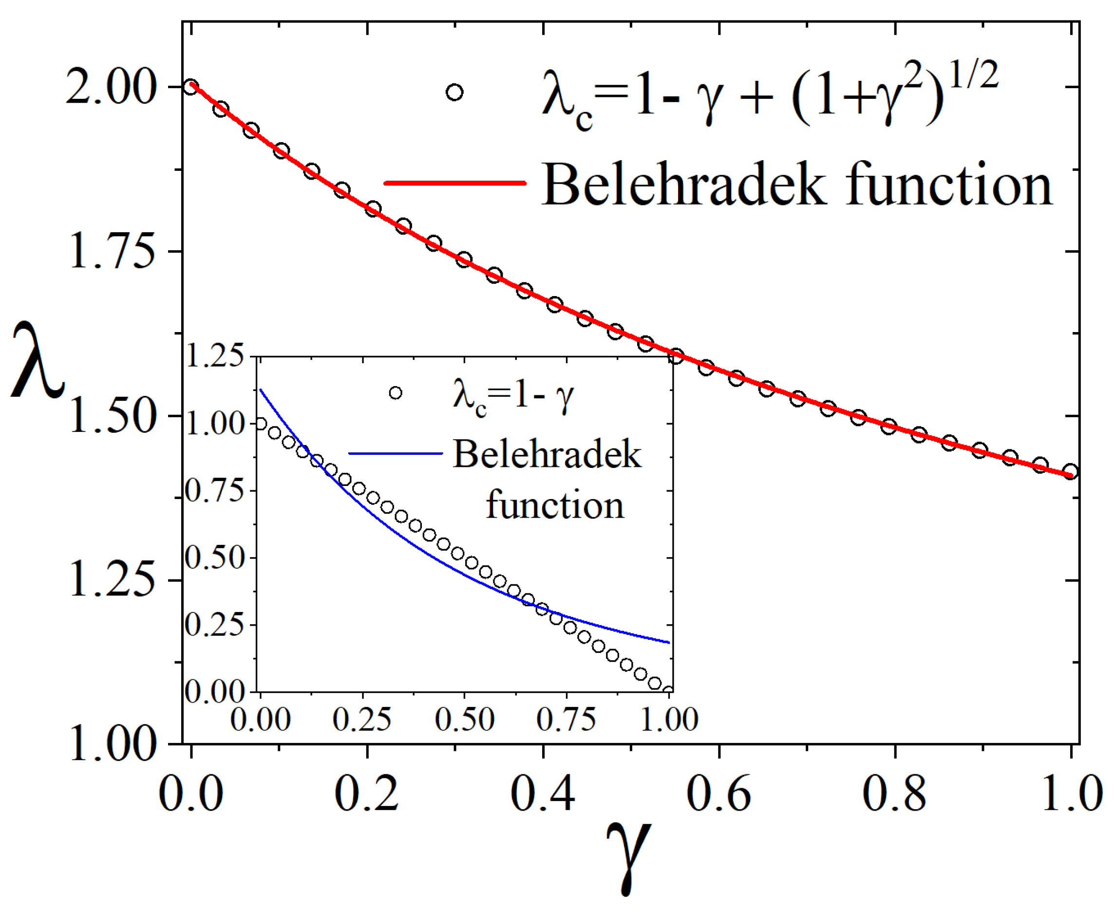
2. Mean-Field Approximation and Pedagogical Arguments

In the one-dimensional case, the transition rate can be expressed as [15]
ω ( σ i 1 σ i | σ i 1 , σ i + 1 ) = λ 2 ( 1 σ i ) ( σ i 1 + σ i + 1 ) + σ i
for the site i from state σ i to state 1 σ i , where σ i = 1 (•) denotes an active site and σ i = 0 (∘) denotes an inactive site. We can verify that ω ( | , ) = λ and ω ( | , ) = ω ( | , ) = λ / 2 and ω ( ) = 1 . When these rates are converted into probabilities, we obtain exactly the probabilities of the CP, since p ( ) ( ) = ω ( | , ) Z , p ( ) ( ) = ω ( | , ) Z = p ( ) ( ) = ω ( | , ) Z , and p ( ) ( ) = ω ( ) Z , which gives exactly the probabilities reported in the first section.
The master equation says that
d P ( σ , t ) d t = i = 1 L ω 1 σ i σ i P σ , t ω σ i 1 σ i P σ , t
with σ ( σ 1 , σ 2 , σ i 1 , σ i , σ i + 1 , , σ N ) and σ σ 1 , σ 2 , σ i 1 , ( 1 σ i ) , σ i + 1 , , σ N , where similarly ω 1 σ i σ i = λ 2 σ i ( σ i 1 + σ i + 1 ) + 1 σ i . For the simplicity of notation, we removed the conditional symbol of Equation (1). We have σ j = σ σ j P ( σ , t ) and, differentiating it with respect to time, we obtain
d σ j d t = σ σ j d P ( σ , t ) d t = i = 1 L σ σ j ω 1 σ i σ i P σ , t i = 1 L σ σ j ω σ i 1 σ i P σ , t = σ ( 1 σ j ) ω σ j 1 σ j P σ , t σ σ j ω σ j 1 σ j Pr σ , t = ( 1 2 σ j ) ω σ j 1 σ j .
Thus,
d σ j d t = ( 1 2 σ j ) λ 2 ( 1 σ j ) ( σ j 1 + σ j + 1 ) + σ j = σ j 2 σ j 2 + 1 2 λ σ j 1 + 1 2 λ σ j + 1 3 2 λ σ j σ j 1 3 2 λ σ j σ j + 1 + λ σ j 2 σ j 1 + λ σ j 2 σ j + 1 .
For the CP model, σ j = 0 , 1 , and therefore σ j 2 = σ j . From this, it follows that
σ j 2 = σ j = ρ ,
and, in addition, we have
σ j 2 σ j 1 = σ j σ j 1 or σ j 2 σ j + 1 = σ j σ j + 1 .
By using the site mean-field approximation, this leads to
σ j σ j 1 σ j σ j 1 = ρ 2 σ j σ j + 1 .
Thus, we obtain
d ρ d t = ( λ 1 ) ρ λ ρ 2 .
Finally, we incorporate the external diffusive effects into the equation. To this end, we adopt an empirical approach to illustrate how such effects might manifest. At low densities, diffusion should be highly sensitive to increases in the density of active sites, as greater mobility enhances the chances for inactive (or healthy) particles to become active (or infected). This effect is expected to grow proportionally with density up to a certain point, beyond which mobility becomes less sensitive, approaching saturation as ρ 1 . Naturally, no diffusion is expected at the extremes ρ = 0 and ρ = 1 . These considerations motivate the introduction of an empirical term of the form
h diff ( ρ ) = D ρ ( 1 ρ )
in Equation (6), where D is a constant related to the mobility of the particles, that is, the probability of diffusion.
In a recent study, some authors revealed that, in nightclub dynamics [16], there is an optimal crowd density to maximize profits, as people can reach the bar counter more easily due to faster diffusion. This is directly related to a term of this kind, as it reflects the efficiency of customer mobility within the nightclub, thus motivating our approach. So, we add this term ad hoc in Equation (6) with the following result:
d ρ d t = ( λ 1 ) ρ λ ρ 2 + D ρ ( 1 ρ ) = λ 1 + D ρ ( D + λ ) ρ 2
The solution of this equation is given by
ρ ( t ) = λ 1 + D ρ 0 e λ 1 + D t λ 1 + D ( D + λ ) ρ 0 + ( D + λ ) ρ 0 e λ 1 + D t
where ρ 0 = ρ ( 0 ) . In the steady state, d ρ d t = 0 , and then
ρ = λ 1 + D ( D + λ )
Thus, we can establish a dependence of λ C on D :
λ C = 1 D
which suggests that, when D increases, λ C decreases. It is interesting to observe that, in the vicinity of the criticality, λ λ C = 1 D , and, therefore, e λ 1 + D t 1 + λ 1 + D t :
ρ ( t ) λ 1 + D ρ 0 1 + λ 1 + D t λ 1 + D + ( D + λ ) ρ 0 λ 1 + D t ρ 0 1 + ( D + λ ) λ 1 + D ρ 0 λ 1 + D t t 1 , when t
This simple MF analysis aims to determine how λ C depends on the diffusion in the case of short-range, one-dimensional contact. In this work, we study the CP model by introducing diffusion into the nearest-neighbor CP defined in the previous section. Our diffusion model randomly selects a site, and a replacement with its nearest neighbor is performed with probability 0 γ 1 , where γ is related to D in the MF regime. The goal is to explore how λ C decays as a function of γ . However, unlike the simple linear relationship in Equation (10), this paper addresses the nature of this decay.
To determine such behavior, we use two techniques:
  • Optimization of the coefficient of determination of temporal power laws, proposed in Ref. [13];
  • Spectral analysis of correlation matrices constructed from multiple realizations of the CP, following the method presented in Ref. [14].
We investigated whether both methods, which rely on the time evolution of the active site density, produce the same underlying physics. The first approach considers averages over different time series, while the second one examines the spectral properties of matrices built from magnetization trajectories.

3. Simulation and Methods

In this work, our order parameter is the density of active particles ρ which, for the i-th sample and at the t-th MC step, can be defined by the matrix element
ρ i , t = 1 L k = 1 L s k ( i ) ( t ) ,
where s k ( i ) ( t ) is 0 if the site k is inactive and 1 otherwise, and L is the size of the system. From this quantity, we explore different approaches to study the one-dimensional CP with diffusion by means of nonequilibrium MC simulations. At each step, a site is chosen randomly with probability 1 / L . If the site is active, it may become inactive, and, if inactive, it may become active, depending on its neighborhood, following the transition probabilities defined in Section 1. One MC step consists of L randomly chosen sites undergoing possible transitions. Next, we account for particle diffusion: in this case, L sites are also randomly selected, each one with the same probability 1 / L . To address the diffusion process, each chosen site exchanges position with one of its two nearest neighbors (chosen at random) with probability γ .
We perform a total of N s a m p l e independent time evolutions, each consisting of N s t e p s MC steps.
To determine λ c as a function of γ , we employ two methods. The first one is based on optimizing power laws [13], where the best fit of the power-law occurs at λ = λ C . The second one is the espectral method, which identifies λ C as the value where the average eigenvalue of correlation matrices reaches a minimum, following the methodology described in Ref. [14].

3.1. First Method: Optimization of Power Laws by the Coefficient of Determination

Our first method involves averaging over different system evolutions or across N s a m p l e s independent simulations:
ρ ( t ) = 1 N s a m p l e i = 1 N s a m p l e ρ i , t
Unlike equilibrium systems, where spatial scaling is often the primary concern, nonequilibrium systems require both temporal and spatial scaling to be considered. This is particularly evident in systems with absorbing states, where a universal scaling relation emerges. This relation, which has significant implications, dictates that the density of active sites must follow the scaling law dependent on initial conditions [3,4,5]:
ρ ( t ) t β / ν f ( ( λ λ C ) t 1 / ν , t d / z L d , ρ 0 t β / ν + θ ) ,
where ρ 0 = ρ ( 0 ) is the initial density of active sites and d is the spatial dimension. The indices z = ν / ν and θ = d z 2 β ν are dynamic critical exponents, while β , ν , and ν are static critical ones.
The quantity λ λ C represents the distance from the critical point and governs the algebraic behavior of two independent correlation lengths: the spatial correlation length, ξ ( λ λ C ) ν , and the temporal correlation length, ξ ( λ λ C ) ν . At criticality ( λ = λ C ), different critical exponents can be estimated from Equation (13) by considering different initial conditions at the beginning of the simulations ( t = 0 ). In the context of time-dependent MC simulations, starting from an initial density ρ = ρ 0 , the following crossover of power laws is expected:
ρ ( t ) ρ 0 t θ if t m i c < t < ρ 0 ν d ν β t δ if ρ 0 ν d ν β t ,
with
δ = β ν .
We focus on the second power law in Equation (14). To derive this power law directly, we begin by initializing the system with ρ 0 = 1 . In this case, the decay follows a power law of the form ρ ( t ) t δ , which is observed at λ = λ c . For λ λ C , an exponential behavior is observed, consistent with the MF analysis that we developed above and summarized in Equation (9).
To pinpoint the critical parameters, we employ a straightforward yet highly effective statistical method for monitoring temporal power laws within time-dependent MC simulations: the coefficient of determination (COD) [17]. This approach recognizes that there are two sources of variation when fitting experimental data linearly: the explained variation and the unexplained one. The total variation is the sum of both variations, and the quality of the linear fit is quantified by the ratio of explained variation to total variation, yielding a COD value (denoted as r) between 0 and 1. A higher COD value indicates a better linear fit.
The method used in this work is based on the approach introduced by da Silva, Drugowich, and Martinez in their study of nonequilibrium statistical mechanics [13]. In that work, they employed the COD in the linearization of the time evolution of averaged magnetizations to localize the critical parameters of the generalized Ising model. Although originally developed for this specific context, this method is generalizable and has been applied successfully to various other models (see, for example, [18]).
We start by computing the average log densities, ln ρ ( t | λ , γ ) , across multiple runs. For each parameter pair ( λ , γ ) , we then determine the coefficient of determination, r, as follows:
r ( λ , γ ) = t = N min N s t e p s ( ln ρ ( t | λ , γ ) ¯ a b ln t ) 2 t = N min N s t e p s ( ln ρ ( t | λ , γ ) ¯ ln ρ ( t ) ) 2 .
Here, the overline indicates an additional averaging step:
ln ρ ( t | λ , γ ) ¯ = 1 N s t e p s t = N min N s t e p s ln ρ ( t ) .
The values N s t e p s and N min correspond to the total number of MC steps performed and the number of initial steps discarded during equilibration, respectively. The optimal parameters are then determined via marginalization:
λ C ( γ ) arg max λ min λ λ max { r ( λ | γ ) } ,
that is, for a fixed γ , we vary λ to find the value that maximizes r. The parameters a and b correspond to the intercept and slope, respectively, of the linear function. When initialized with ρ 0 = 1 , b equals δ at the critical point. The intervals [ λ min , λ max ] are selected to ensure proper refinement.
As defined in Equation (16), r quantifies the ratio of explained variation to total variation. Near the critical point λ = λ C , r approaches unity ( r 1 ), indicating that ρ ( t ) follows a power-law distribution. This power-law behavior manifests as a linear relationship on a log-log scale. Conversely, far from the critical point, ρ ( t ) deviates from power-law scaling, as described in Equation (14), resulting in r 0 .

3.2. Second Method: Spectral Analysis of Correlation Matrices
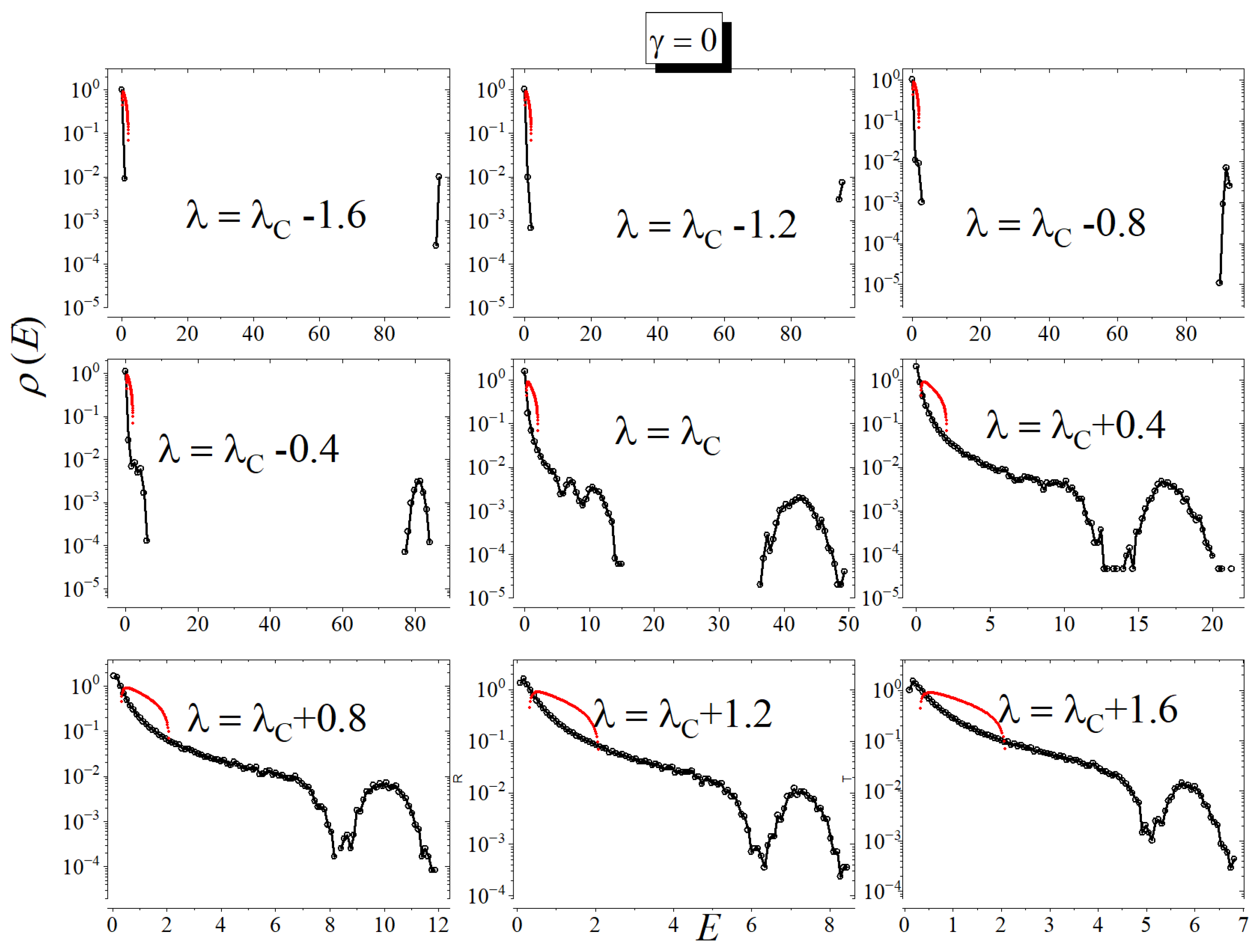
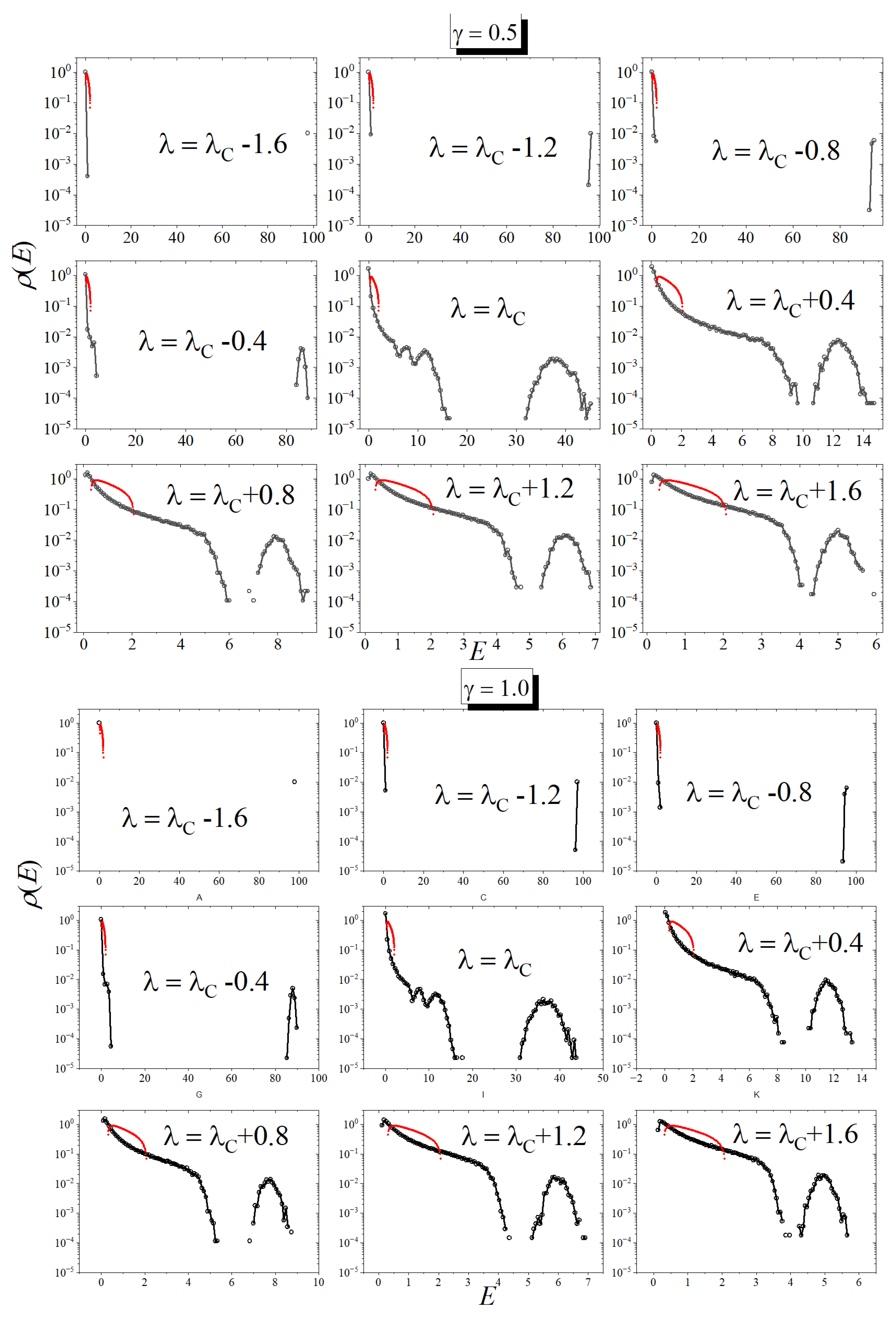
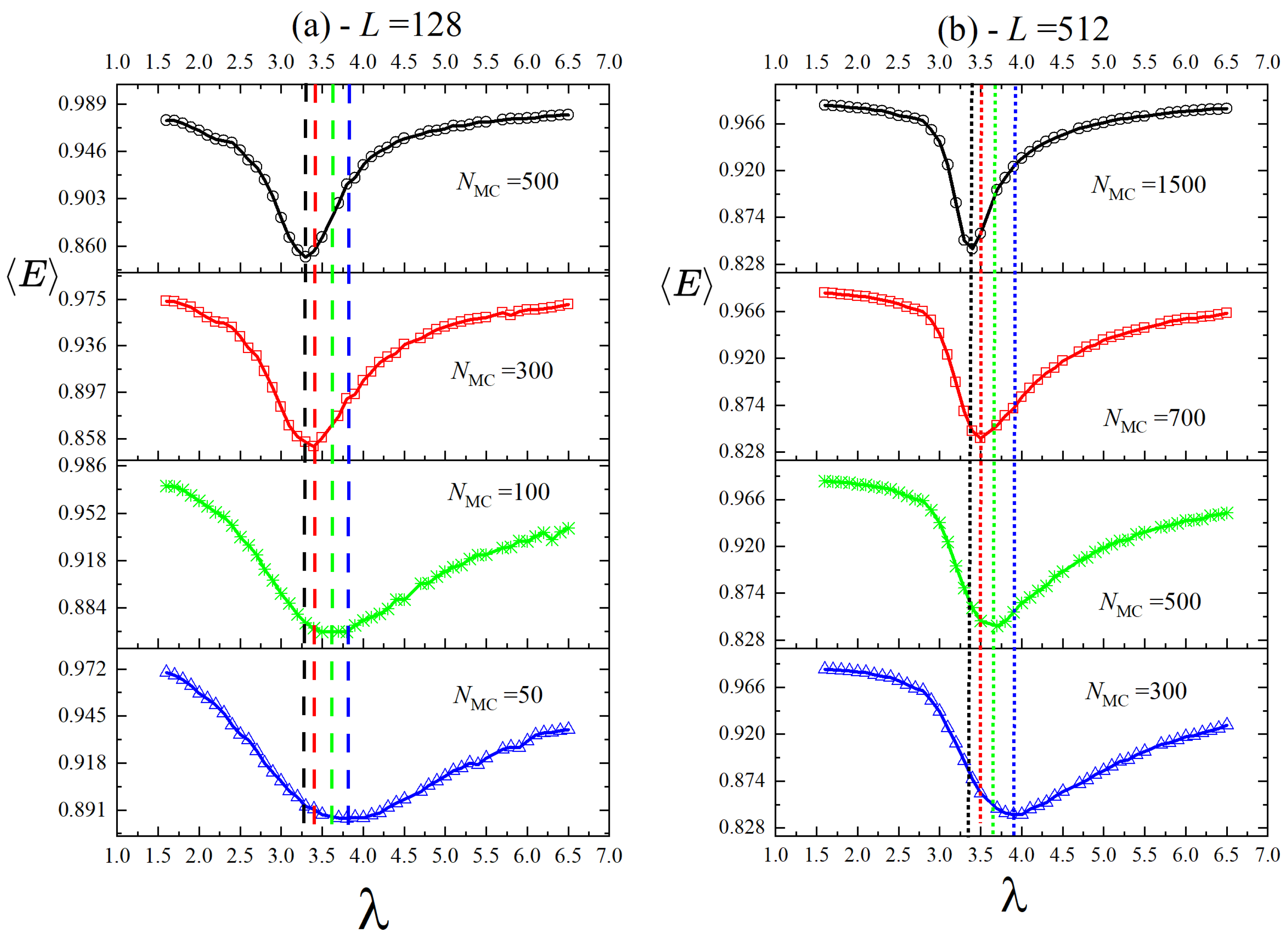
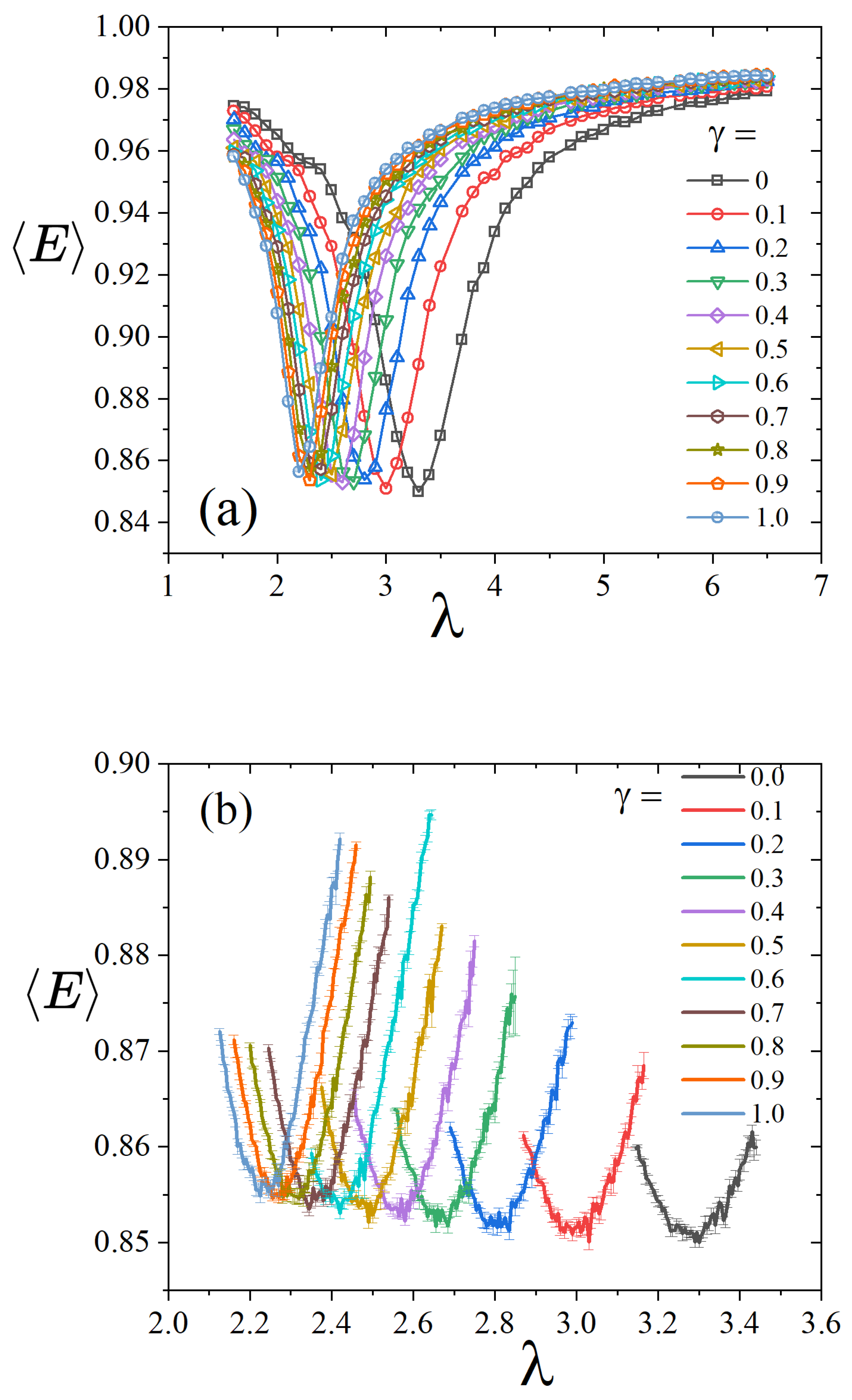
The second method builds on the methodology introduced in Ref. [14], where a cross-correlation matrix C is constructed from time series iterations of a given observable—such as generalized momentum, generalized position, or magnetization per particle. Although prior works, including Refs. [14,19,20], have explored the method by using the eigenvalues of such matrices to detect phase transitions in spin systems, this technique has also proven to be effective in quantifying genuine correlations in financial markets. In econophysics, for instance, financial returns serve as the observable [21,22,23,24,25].
Interestingly, the foundational approach traces back to Wishart’s 1928 work [26] on what later became known as Wishart ensembles in statistics—predating the famous random matrix ensembles of Wigner and Dyson [27,28,29] in statistical mechanics. Despite its long history, this methodology still holds unexplored potential for novel applications.
In this work, we instead focus on the density of active sites as the observable. The elements of the cross-correlation matrix C are defined as
C i j = ρ i ρ j ρ i ρ j σ ρ i σ ρ j
where the averages and standard deviations are calculated from two time series of length N s t e p s : ρ k , 0 , ρ k , 1 , , ρ k , N s t e p s 1 , where k = i , j = 1 , , N s a m p l e .
The expectation values are given by
ρ k = 1 N s t e p s p = 0 N s t e p s 1 ρ k p , ρ i ρ j = 1 N s t e p s p = 0 N s t e p s 1 ρ i p ρ j p
and the standard deviation σ ρ k is calculated via
σ ρ k = 1 ( N s t e p s 1 ) p = 0 N s t e p s 1 ( ρ k p ρ k ) 2 ρ k 2 ρ k 2 .
It is important to note that the matrix C , of dimension N s a m p l e , can be obtained from the standardized time-evolution matrix M :
M = ρ 10 ρ 1 σ ρ 1 ρ 20 ρ 2 σ ρ 2 ρ N s a m p l e 0 ρ N s a m p l e σ ρ N s a m p l e ρ 11 ρ 1 σ ρ 1 ρ 21 ρ 2 σ ρ 2 ρ N s a m p l e 1 ρ N s a m p l e σ ρ N s a m p l e ρ 1 N s t e p s 1 ρ 1 σ ρ 1 ρ 2 N s t e p s 1 ρ 2 σ ρ 2 ρ N s a m p l e N s t e p s 1 ρ N s a m p l e σ ρ N s a m p l e
This allows us to verify that
C = 1 N s t e p s M t M .
It is known that, if ρ i , 0 , ρ i , 1 , , ρ i , N s t e p s 1 are a set of independent random variables, we are in the context of the real Wishart ensemble [30,31]. In that case, the joint probability distribution of the eigenvalues is expected to be given by
P ( E 1 , , E N s a m p l e ) = 1 Z e H ( E 1 , , E N s a m p l e ) ,
where
Z = ... d E 1 d E N s a m p l e e H ( E 1 , , E N s a m p l e )
and
H ( E 1 , , E N s a m p l e ) = H auto ( E 1 , , E N s a m p l e ) + H int ( E 1 , , E N s a m p l e ) ,
corresponding to a Hamiltonian of a Coulomb gas with logarithmic repulsion
H int ( E 1 , , E N s a m p l e ) = i < j ln E i E j ,
and the term
H auto ( E 1 , , E N s a m p l e ) = N s t e p s 2 i = 1 N s a m p l e E i ( N s t e p s N s a m p l e 1 ) 2 i = 1 N s a m p l e ln E i ,
attracts the particles to the origin, with E 1 , , E N s a m p l e 0 . Since N s t e p s > N s a m p l e , we have
E > ( N s t e p s N s a m p l e 1 ) N s t e p s ln E .
In the case of potentials described by Equations (25) and (26), the density of states is defined by
σ ( E ) = 0 0 0 P ( E , E 2 , E N s a m p l e ) i = 1 N s a m p l e d E i
following the well-known Marchenko–Pastur (MP) law [32,33]:
σ M ( E ) = N M C 2 π N s a m p l e ( E E ) ( E + E ) E if E E E + 0 otherwise ,
where
E ± = 1 + N s a m p l e N M C ± 2 N s a m p l e N M C .
We construct matrices by examining the evolution of active sites of the CP model. A key quantity to track is the deviation of the density of states from the non-correlated scenario, as defined by σ M ( E ) in Equation (28). This deviation is captured by the first moment of σ ( E ) , given by E [ E ] = 0 E σ ( λ ) d λ . Its estimator is derived from the numerical density of states:
E = i = 1 N i n t σ N ( E i ) E i i = 1 N i n t σ N ( E i ) ,
where N i n t represents the number of bins used to compute the numerical density of states σ N ( E i ) , which may differ from the expression in Equation (28). This leads to a change in the function H auto ( E 1 , , E N s a m p l e ) from that given in Equation (28), introducing gaps in the density of states. These gaps are reflected in the first moment E or higher moments σ ( E ) . Our previous work has demonstrated that extreme values of E are closely associated with phase transition points in spin systems [14] and chaotic-to-stability transitions in chaotic maps [34].
An important distinction here is that, unlike Ising systems, where we expect σ N ( E ) σ M ( E ) as T , as described in Equation (28), or at least a good approximation at this limit, as shown in Ref. [14], this does not necessarily hold for the CP model. In the CP model, as λ , we observe p ( ) ( ) 1 , p ( ) ( ) = p ( ) ( ) 1 / 2 , and p ( ) ( ) 0 . The system tends to evolve toward a state where all sites are active. On the other hand, when λ 0 , p ( ) ( ) = p ( ) ( ) = p ( ) ( ) 0 and p ( ) ( ) 1 , causing all sites to become inactive.
In the Ising model, for instance, at T , p ( s i = + 1 ) = p ( s i = 1 ) = 1 2 , and the time evolution of the magnetization, m ( t ) = 1 N i = 1 N s i ( t ) , follows a Gaussian distribution that is uncorrelated with any other evolution. Therefore, in this case, we expect the system to recover the MP law, as given by Equation (28). However, in the CP model, a gap dynamics (different from Ising systems) must still be maintained to ensure that the minimum average eigenvalue reaches a minimum at λ = λ C .

4. Results

Now, we present our results for the estimates of the critical value as a function of mobility using both methods previously described: Method 1—Optimization of the power laws, and Method 2—Spectral analysis of correlation matrices.

4.1. Method 1

We begin by performing MC simulations to determine the critical parameters for different diffusion settings. The range of λ min spans from 1.5 to 3.5 , with a resolution of Δ λ = 0.01 . We simulate the CP with mobility for systems of size L = 1024 , running a total of N s t e p s = 500 MC steps for each evolution. The first N min = 30 MC steps are discarded, and we then average the results of ρ ( t | λ , γ ) over N s a m p l e = 2000 different time evolutions for each mobility value γ . Just as a test of our approach and for fast comparison with results presented in the literature, when considering γ = 0 , we obtain δ = β ν 0.159 for a single seed, which is very close to the known estimates of the one-dimensional directed percolation δ = 0.159464 ( 6 ) [4].
Next, we optimize the process by calculating the coefficient of determination r obtained from the linear fit of ρ ( t | λ , γ ) × t in log-log scale for each of the 200 λ -values tested, across 11 different values of γ , ranging from γ = 0.0 to γ = 1.0 ( Δ λ = 0.1 ). The results for r as a function of λ are shown in Figure 1.
As observed, λ C decays as a function of γ , in (qualitative) agreement with the prediction of the MF approximation, although not exhibiting the same simple behavior (i.e., λ C = 1 D ) found there. It is important to note that this is not directly comparable, as the dependence of γ on D is not known. Regarding the fits of λ C as a function of γ , relevant fits are discussed in Section 4.3. First, we demonstrate that Method 2 corroborates the results obtained from Method 1, showing that both methods can be used to localize the critical parameters of the contact process (CP) model with mobility.

4.2. Method 2

In the second method, we construct correlation matrices with N s a m p l e = 100 different time evolutions. Unlike the approach used for the Ising model as well as other up–down symmetry models, we set ρ 0 = 1 here. It is important to note that, in this case, there is no order–disorder transition, and the minimal density for evolution is ρ 0 = 1 / L , which has a different effect compared to m 0 = 0 in the up–down symmetry models.
In addition, we built histograms from N r u n = 1000 different random matrices by considering L = 2 7 sites (fewer than in the previous method, which is consistent with the results obtained in Ref. [14]—see Figure 3 of that reference) and N s t e p s = 500 , yielding a total of 10 5 eigenvalues. Simulations were performed for different values of γ . It is interesting to observe how the density of states, σ ( E ) , behaves for various values of λ (it is important to construct these histograms, rather than calculating the averages directly, for the method to work properly). Unlike the observation in up–down symmetry systems, where high temperatures lead to a migration of the density of states toward the MP law, in the CP, the result shows that migration does not occur, as can be seen in Figure 2 for different values of γ .
As previously noted, when λ or λ 0 , the system exhibits two distinct absorbing states due to its symmetry. In one case, all particles are active, while, in the other, all particles are inactive. In both scenarios, the system necessarily deviates from the MP law. The red curves in the plots demonstrate that the density of states significantly differs from the MP law in these situations, a characteristic that distinguishes this system from Ising-like models.
Although there is a gap structure in the eigenvalues that resembles that of Ising-like models, we cannot establish a direct link between these gaps and the phase transition simply by observing the eigenvalue bulk and gap dynamics. It is important to note that, even in Ising-like systems, the dynamics of gap closing alone do not fully explain phase transitions based on these matrices. However, fluctuations in the histograms (density of states) of both Ising-like models [14] and the current CP seem to reliably predict the existence of critical points, regardless of our understanding of the bulk and gap dynamics. This observation warrants a more in-depth theoretical exploration, though this is beyond the scope of the current study.
For example, refer to Figure 3, where we used the density of states to calculate the average eigenvalue E as a function of λ for two lattice sizes: (a) L = 128 and (b) L = 512 , with γ = 0 , without any loss of generality. We observe that the method works well for small systems, as we used only L = 2 7 sites, with results depending on the adjusted N s t e p s . Larger systems, however, require significantly more computational effort, as indicated by Figure 3b. Based on Equation (29), we analyze the results for L = 128 and L = 512 sites. Drawing from the hypothesis presented in previous works [14,34], where a minimum in the average eigenvalue suggests the existence of a critical point, we explore how this method performs for these two system sizes.
For each lattice, we varied N s t e p s . Observations show that, for L = 128 with N s t e p s = 500 MC steps, we obtained λ 3.29 , a value very close to the critical point expected for γ = 0 . However, for L = 512 , a significantly higher computational cost was required, with N s t e p s = 1500 MC steps. This suggests that using L = 512 is unnecessary, as the correlation matrix method works efficiently for L = 128 . The problem is well-calibrated for this system size using N s t e p s = 500 MC steps.
Thus, for L = 128 , we calculated E as a function of λ for various γ values. Initially, we used Δ λ = 0.1 , referred to as the coarse-grained stage. The minimal value of E indicates that the critical temperature varies as γ changes (see Figure 4a).
After an initial rough localization, we then proceed with a finer refinement using Δ λ = 0.005 (fine-scale stage). The behavior of E as a function of λ is presented in Figure 4b. Despite averaging across five different seeds, the process remains notably noisy. However, we successfully determined the minimum point, λ C , by averaging results from the different seeds. These findings will now be compared to those obtained using the power-law optimization method (Method 1).

4.3. Comparison Between the Methods

In Figure 5, we show λ C as a function of γ using the two methods described in this manuscript. The results appear to be in good agreement. The square markers represent the method where we calculated the minimum of the average eigenvalue of correlation matrices constructed from the time evolution of the density of active sites (Method II), while the circular markers correspond to the method where we observed the temporal power-law averages across different time evolutions.
We observe a non-trivial decay of λ C with γ , which differs from the behavior seen in the MF regime, where λ c = 1 D . After empirically testing several candidate functions, we found that the Belehradek function, widely known in the literature, provides a good fit:
λ C = a ( γ b ) c
where we determined a 2.33 , b 0.16 , and c 0.19 , yielding an excellent fit quality with a coefficient of determination (COD) of approximately 0.999667 .
The Belehradek equation is traditionally associated with temperature effects in biological processes (e.g., see [35]). In this context, we adopt it in an entirely empirical manner. Here, we do not intend to draw any comparison with a biological process; we simply use the name to refer to a specific power function characterized by three parameters.
The key point here is that both methods are in agreement, providing a strong fit that describes how the critical parameters of the CP change with mobility, which follows the Belehradek function. This suggests that the results qualitatively support our simple MF model, where λ c decays linearly with D, a parameter that is related to the mobility of the system γ .
It is worth noting that, although several studies have examined diffusion in the CP, making a meaningful comparison with our results is not straightforward. To the best of our knowledge, none of these works have determined the critical parameter as a function of the mobility parameter, as we have done here using time-dependent MC simulations applied to our version of the model on the lattice.
On the other hand, a qualitative comparison is possible. For example, in Figure 1 of Reference [9] and Figure 6 of Reference [11], the authors observe that the annihilation rate α , which in our manuscript corresponds to 1 1 + λ , increases as a function of the diffusion rate D. In their studies, D varies from 0 to 1, which corresponds to our mobility probability γ . Therefore, if d α d D > 0 , we must show that d λ d D = d λ d γ < 0 , since we observe a decrease in λ as a function of γ . Applying the chain rule
d α d λ d λ d D = 1 ( 1 + λ ) 2 d λ d γ > 0
consequently, it must hold that
d λ d γ < 0
This confirms that our result is consistent with findings in the literature.
However, following the helpful suggestion of the anonymous referees, concerning the contact process discussed in [36] that uses a pair-approximation mean-field approach, by comparing their diffusion parameters with the parameters used in this work, we can conclude the following:
λ C = 1 γ + 1 + γ 2 .
From a pedagogical perspective, it is interesting to observe that the first part of this expression, 1 γ , is exactly what our very simple approximation yields. The second term, 1 + γ 2 , which arises from the pair approximation, plays a crucial role. Why is this important? As shown in our manuscript, MC simulations indicate that λ C is well-fitted by a power-law-type function known as the Belehradek function: λ C = a ( γ b ) c . Naturally, our simple mean-field approximation, which captures only the 1 γ term, does not match this behavior well. However, when we include the second term, the fit improves significantly, yielding coefficients a 1.76 , b = 0.73 , and c 0.41 . This shows that our approximation represents just the first part, which is then completed by the pair approximation—though with coefficients that differ slightly from those obtained via MC simulations. This demonstrates that our approximation serves as an initial step, further refined by the pair approximation, and ultimately validated by our MC simulations using two different methods.
Please refer to Figure 6, where the pair-approximation model demonstrates a good fit with the Belehradek function, which also closely matches our Monte Carlo (MC) simulations.

4.4. Brief Discussion About the Computational Complexity of the Methods

It is important to note that both methods perform well, even with a small number of MC steps. In models with a defined Hamiltonian, this behavior is typically described as avoiding critical slowing down. However, in the case of an intrinsically nonequilibrium model like ours, it is more accurate to say that the system remains far from its steady state. The computational complexity of the proposed methods is determined by three key components:
  • Sampling: The analysis requires N sample independent realizations of the order parameter’s time evolution (e.g., the density of active sites);
  • Time Evolution: Each realization comprises a time series of N steps MC steps;
  • System Operations: Each MC step involves N = L elementary operations, where L represents the system size.
Therefore, the time complexity for the first method scales as
C 1 = O ( N sample × N steps × L ) .
The second method analyzes the same quantities as the first approach, but with one additional step: the diagonalization of an N sample × N sample matrix. This leads to a modified complexity:
C 2 = O ( N sample 3 × N steps × L )
Why, then, should one use Method 2? The answer can be divided into two parts. First, Method 2 investigates the existence of criticality in the spectrum of a certain matrix, which is significant from a theoretical perspective, since we show that spectra respond to a phase transition, which by itself is interesting. As a computational method, its main advantage is that it requires much smaller values of both N sample and especially L, when compared to Method 1. At first glance, the performance of Method 2 may appear considerably worse than that of Method 1, as indicated by the values of C 2 and C 1 , respectively. However, it is important to recognize that the parameters used in each case are fundamentally different. Method 2 operates on much smaller lattices and uses fewer samples. While both methods employ N steps = 500 , Method 1 requires L 1 = 1024 and N sample ( 1 ) = 1000 , whereas Method 2 uses L 2 = 128 and N sample ( 2 ) = 100 . As a result, the estimated computational costs, based on the operations performed, are
C 1 1000 × 1024 = 1.024 × 10 6 , and C 2 = 100 4 × 128 = 1.28 × 10 10 .
Things may seem at their worst, but we must look beyond and stay hopeful! A key observation is that, in Method 2, the value of N sample appears to have a negligible impact on the results. Across all models studied so far—including one- and two-dimensional systems—we have consistently used N sample = 100 , suggesting that this parameter can be treated as essentially fixed. Therefore, the complexity of Method 2 should be reconsidered as primarily dependent on L, rather than on both N sample and L. This behavior has been previously documented in studies of the Potts model, transitions to chaos, aging effects, and related phenomena (see, for example, [14,34,37,38,39]). In all these studies, Method 2 was applied using N sample = 100 . Consequently, the relevant factor for complexity in this approach is the system size L, which remains significantly smaller, asymptotically, than that required in conventional MC simulations, as also shown by the finite-size scaling analysis in [14].
Finally, we emphasize that our goal is not to compare or rank the methods, but to demonstrate that, whether one analyzes the time evolution of the spectrum of random matrices or directly examines power laws, the conclusions are consistent. Our central focus is to understand how criticality evolves under diffusion, regardless of the specific method employed. However, we would like to emphasize that these points should be considered in such heuristics. Certain aspects of the methods’ complexity warrant deeper investigation, as there are practical elements that are not yet fully understood.

5. Conclusions

We studied the contact process using two nonequilibrium methods: optimization of temporal power laws and spectral analysis of correlation matrices, both based on N s a m p l e evolutions of the density of active particles. Specifically, we examine how the critical rate λ C varies with the mobility of particles γ . Our results demonstrate that λ C decays with γ following a Belehradek function, with both methods presenting good agreement.
These findings qualitatively support the MF regime, where λ c is expected to decay with mobility, which in this case is represented by the parameter D.

Author Contributions

Conceptualization, R.d.S., E.V.F., H.A.F. and P.F.G.; Methodology, R.d.S., E.V.F., H.A.F. and P.F.G.; Software, R.d.S. and E.V.F.; Validation, R.d.S., E.V.F., H.A.F. and P.F.G.; Formal analysis, R.d.S.; Investigation, R.d.S., E.V.F., H.A.F. and P.F.G.; Resources, R.d.S.; Data curation, R.d.S.; Writing—original draft, R.d.S.; Writing—review & editing, R.d.S., E.V.F., H.A.F. and P.F.G.; Visualization, R.d.S.; Supervision, R.d.S.; Project administration, R.d.S.; Funding acquisition, R.d.S. All authors have read and agreed to the published version of the manuscript.

Funding

This research was funded by CNPq under grant number 304575/2022-4.

Data Availability Statement

The data presented in this study are openly available and can be directly required by the authors by e-mail: rdasilva@if.ufrgs.br.

Acknowledgments

R. da Silva would like to express gratitude to M. J. de Oliveira and R. Dickman for their valuable insights regarding the contact process. The authors also thank the anonymous referees for pointing out the interesting paper by Ben-Avraham and Köhler, which provides an important clarification on the extension of the mean-field approximation in relation to numerical results.

Conflicts of Interest

The authors declare no conflicts of interest.

References

  1. Harris, T.E. Contact interactions on a lattice. Ann. Prob. 1974, 2, 969. [Google Scholar] [CrossRef]
  2. Ligget, T.M. Interacting Particle Systems; Springer: New York, NY, USA, 1995. [Google Scholar]
  3. Marro, J.; Dickman, R. Nonequilibrium Phase Transitions; Cambridge University Press: Cambridge, UK, 1999. [Google Scholar]
  4. Hinrichsen, H. Non-equilibrium critical phenomena and phase transitions into absorbing states. Adv. Phys. 2000, 49, 815. [Google Scholar] [CrossRef]
  5. Henkel, M.; Pleimling, M. Non-Equilibrium Phase Transitions, Volume 2: Ageing and Dynamical Scaling Far from Equilibrium; Springer: Dordrecht, The Netherlands, 2010. [Google Scholar]
  6. Dickman, R. Nonequilibrium lattice models: Series analysis of steady states. J. Stat. Phys. 1989, 55, 997–1026. [Google Scholar] [CrossRef]
  7. Böttcher, L.; Herrmann, H.J.; Henkel, M. Dynamical universality of the contact process. J. Phys. A Math. Theor. 2018, 51, 125003. [Google Scholar] [CrossRef]
  8. da Silva, R.; Dickman, R.; Drugowich de Felício, J.R. Critical behavior of nonequilibrium models in short-time Monte Carlo simulations. Phys. Rev. E 2004, 70, 067701. [Google Scholar] [CrossRef]
  9. Dantas, W.G.; de Oliveira, M.J.; Stilck, J.F. Revisiting the one-dimensional diffusive contact process. J. Stat. Mech. 2007, P08009. [Google Scholar] [CrossRef]
  10. Dantas, W.G.; de Oliveira, M.J.; Stilck, J.F. Dependence of the crossover exponent with the diffusion rate in the generalized contact process model. Braz. J. Phys. 2008, 38, 94–96. [Google Scholar] [CrossRef]
  11. Fiore, C.; de Oliveira, M.J. Phase transition in conservative diffusive contact processes. Phys. Rev. E 2004, 70, 046131. [Google Scholar] [CrossRef]
  12. Shen, J.; Li, W.; Deng, S.; Xu, D.; Chen, S.; Liu, F. Machine learning of pair-contact process with diffusion. Sci. Rep. 2022, 12, 19728. [Google Scholar] [CrossRef]
  13. da Silva, R.; de Felício, J.R.D.; Martinez, A.S. Generalized Metropolis dynamics with a generalized master equation: An approach for time-independent and time-dependent Monte Carlo simulations of generalized spin systems. Phys. Rev. E 2012, 85, 066707. [Google Scholar] [CrossRef]
  14. da Silva, R. Random matrices theory elucidates the nonequilibrium critical phenomena. Int. J. Mod. Phys. C 2023, 34, 2350061. [Google Scholar] [CrossRef]
  15. Tomé, T.; de Oliveira, M. Stochastic Dynamics and Irreversibility; Springer: Berlin/Heidelberg, Germany, 2014. [Google Scholar]
  16. Stock, E.V.; da Silva, R. Chaos Solit. Fractals 2023, 168, 113117. [Google Scholar] [CrossRef]
  17. Trivedi, K.S. Probability and Statistics with Realiability, Queuing, and Computer Science and Applications, 2nd ed.; John Wiley and Sons: Chichester, UK, 2002. [Google Scholar]
  18. da Silva, R.; Fernandes, H.A.; de Felício, J.R.D. Nonequilibrium scaling explorations on a two-dimensional Z (5)-symmetric model. Phys. Rev. E 2014, 90, 042101. [Google Scholar] [CrossRef] [PubMed]
  19. Vinayak, T.; Prosen, T.; Buca, B.; Seligman, T.H. Spectral analysis of finite-time correlation matrices near equilibrium phase transitions. EPL 2014, 108, 20006. [Google Scholar] [CrossRef]
  20. Biswas, S.; Leyvraz, F.; Castillero, P.M.; Seligman, T.H. Rich structure in the correlation matrix spectra in non-equilibrium steady states. Sci. Rep. 2017, 7, 40506. [Google Scholar] [CrossRef]
  21. Plerou, V.; Gopikrishnan, P.; Rosenow, B.; Amaral, L.N.; Stanley, H. Universal and nonuniversal properties of cross correlations in financial time series. Phys. Rev. Lett. 1999, 83, 1471–1474. [Google Scholar] [CrossRef]
  22. Plerou, V.; Gopikrishnan, P.; Rosenow, B.; Amaral, L.N.; Stanley, H. A random matrix theory approach to financial cross-correlations. Physica A 2000, 287, 374–382. [Google Scholar] [CrossRef]
  23. Stanley, H.E.; Gopikrishnan, P.; Plerou, V.; Amaral, L.A.N. Quantifying fluctuations in economic systems by adapting methods of statistical physics. Physica A 2000, 287, 339–361. [Google Scholar] [CrossRef]
  24. Laloux, L.; Cizeau, P.; Potters, M.; Bouchaud, J.-P. Random matrix theory and financial correlations. Int. J. Theor. Appl. Financ. 2000, 3, 391. [Google Scholar] [CrossRef]
  25. Bouchaud, J.-P.; Potters, M. Theory of Finantial Risks. In From Statistical Physics to Risk Management; Cambridge University Press: Cambridge, UK, 2000. [Google Scholar]
  26. Wishart, J. The generalised product moment distribution in samples from a normal multivariate population. Biometrika 1928, 20, 32–52. [Google Scholar] [CrossRef]
  27. Wigner, E.P. On the Distribution of the Roots of Certain Symmetric Matrices. Ann. Math. 1958, 67, 325. [Google Scholar] [CrossRef]
  28. Dyson, F.J. Statistical theory of the energy levels of complex systems. I. J. Math. Phys. 1962, 3, 140. [Google Scholar] [CrossRef]
  29. Mehta, M.L. Random Matrices; Academic Press: Boston, MA, USA, 1991. [Google Scholar]
  30. Vinayak, T.H. Seligman, Time series, correlation matrices and random matrix models. AIP Conf. Proc. 2014, 1575, 196–217. [Google Scholar]
  31. Livan, G.; Novaes, M.; Vivo, P. Introduction to Random Matrices, Theory and Practice; Springer: Berlin/Heidelberg, Germany, 2018. [Google Scholar]
  32. Marcenko, V.A.; Pastur, L.A. Distribution of eigenvalues for some sets of random matrices. Math. USSR Sb. 1967, 1, 457. [Google Scholar] [CrossRef]
  33. Sengupta, A.M.; Mitra, P.P. Distributions of singular values for some random matrices. Phys. Rev. E 1999, 60, 3389. [Google Scholar] [CrossRef]
  34. da Silva, R.; Prado, S.D. Exploring Transition from Stability to Chaos through Random Matrices. Dynamics 2023, 3, 777–792. [Google Scholar] [CrossRef]
  35. Ross, T. Bělehrádek-type models. J. Ind. Microbiol. 1993, 12, 180–189. [Google Scholar] [CrossRef]
  36. ben-Avraham, D.; Köhler, J. Mean-field (n, m)-cluster approximation for lattice models. Phys. Rev. A 1992, 45, 8358. [Google Scholar] [CrossRef]
  37. da Silva, R.; Filho, E.V.; Prado, S.D.; de Felício, J.R.D. Efficient computational method using random matrices describing critical thermodynamics. Int. J. Mod. Phys. C 2024, 37, 1–30. [Google Scholar] [CrossRef]
  38. da Silva, R.; Prado, S.D. Identifying patterns using cross-correlation random matrices derived from deterministic and stochastic differential equations. Chaos 2025, 35, 033147. [Google Scholar] [CrossRef]
  39. da Silva, R.; Tomé, T.; de Oliveira, M.J. Numerical exploration of the aging effects in spin systems. Phys. Lett. A 2023, 489, 129148. [Google Scholar] [CrossRef]
Figure 1. Coefficient of determination, r, as a function of λ for 1.5 λ 3.5 with Δ λ = 10 2 . The different curves correspond to values of γ ranging from 0 to 1.0 , with increments of 0.1 (i.e., γ = 0 , 0.1 , 0.2 , , 0.9 , 1.0 ).
Symmetry 17 00774 g001
Figure 2. The density of states for γ = 0 , γ = 0.5 , and γ = 1.0 is shown for different values of λ . The red curves represent the MP law for N s t e p s = 500 and N s a m p l e = 100 for comparison, highlighting that, particularly in the CP, the MP law does not play a significant role, differing from what is observed for Kinect Ising systems.
Symmetry 17 00774 g002aSymmetry 17 00774 g002b
Figure 3. Average eigenvalue E as a function of λ is shown for two lattice sizes: (a) L = 128 and (b) L = 512 . For each lattice size, we vary the number of MC steps, N s t e p s . For L = 128 and N s t e p s = 500 , we obtain a result of λ 3.29 , which is already very close to the critical point for γ = 0 . In contrast, for L = 512 , a significantly higher number of steps, N s t e p s = 1500 , is required to achieve a similar level of accuracy, indicating a much higher computational cost.
Symmetry 17 00774 g003
Figure 4. (a) Average eigenvalue E as a function of λ for various values of γ during the coarse-grained stage with Δ λ = 0.1 . (b) Average eigenvalue E as a function of λ for various γ values in the fine-scale regime with Δ λ = 0.005 .
Symmetry 17 00774 g004
Figure 5. Comparison between Method 1 (optimization of power laws) and Method 2 (spectral analysis of correlation matrices). The results are in agreement and also appear to be well-fitted to the Belehradek fit.
Symmetry 17 00774 g005
Figure 6. The Belehradek function is presented, with both the simple mean-field and the pair-approximation mean-field models.
Symmetry 17 00774 g006
Disclaimer/Publisher’s Note: The statements, opinions and data contained in all publications are solely those of the individual author(s) and contributor(s) and not of MDPI and/or the editor(s). MDPI and/or the editor(s) disclaim responsibility for any injury to people or property resulting from any ideas, methods, instructions or products referred to in the content.

