
High Impedance Fault Line Detection Based on Current Traveling Wave Spectrum Symmetry Driving for New Distribution Network

Abstract
1. Introduction
1.1. Background and Challenge
1.2. Existing Research and Comparison
1.3. Primary Focus and Contributions
- New paradigm of spectrum waveform: This approach differs from traditional methods relying on steady-state components, transient signals, or harmonic thresholds. The amplitude–frequency–polarity asymmetry of fault CTW spectra is first used for line selection. Qualitative difference features are extracted via Pisarenko spectral decomposition, eliminating the need for quantitative threshold setting. This solves the sensitivity issues caused by short data windows of new energy and weak fault characteristics.
- Threshold-free clustering mechanism: A spectrum similarity matrix based on Manhattan distance and an improved DBSCAN clustering algorithm are innovatively designed. No empirical thresholds or neutral point current detection are required, achieving 97.5% accuracy under complex grid topologies and new energy fluctuations.
2. CTW Spectrum Fault Line Detection Principle for New Distribution Network
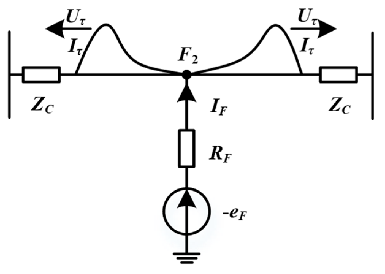
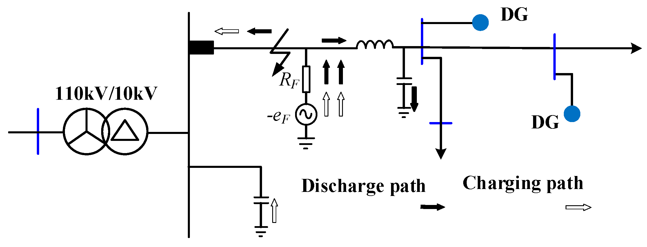
2.1. Generation Mechanism of Fault CTW in New Distribution Network
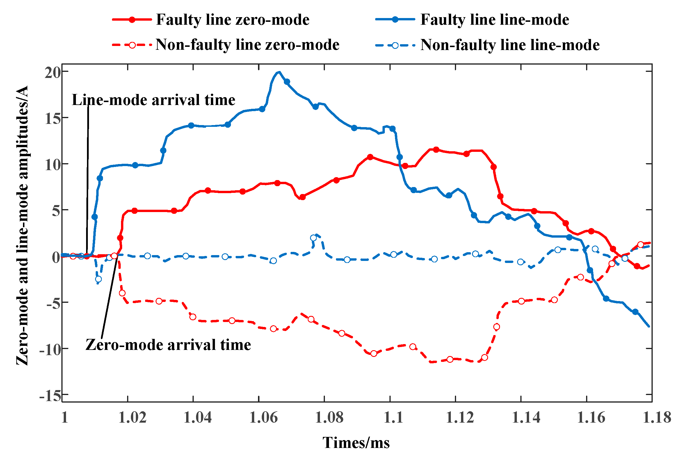
2.2. Traveling Wave Modulus Selection
2.3. Symmetry Analysis of Operating Conditions
2.3.1. Analysis of Balance Parameters Under Symmetric Operating Conditions
2.3.2. Analysis of Unbalance Parameters Under Symmetric Conditions
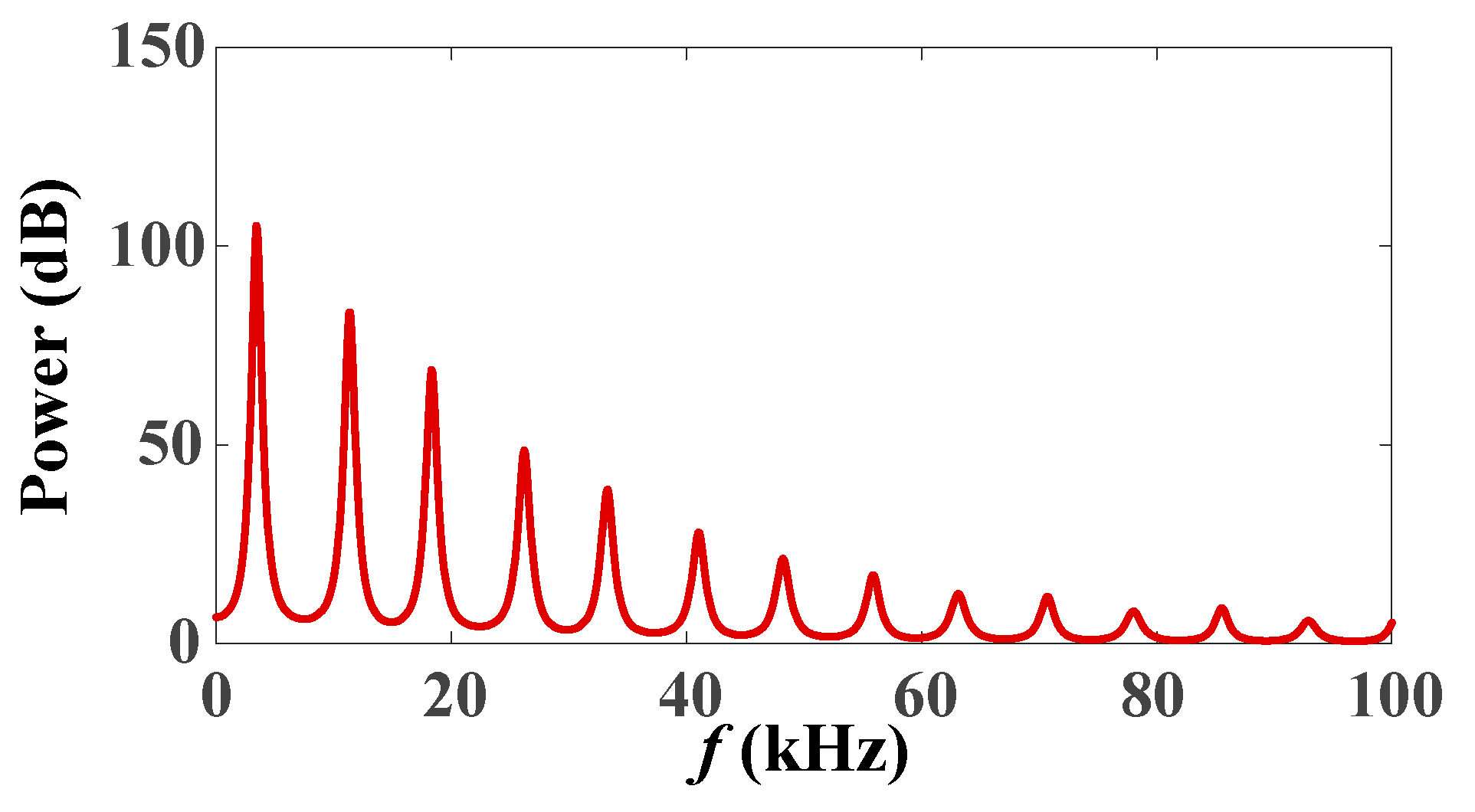
2.4. CTW Spectrum Waveform
3. Multi-Feature Difference Analysis of CTW Spectrum Waveform
3.1. Spectrum Waveform Amplitude Characteristics
3.2. Frequency Characteristics of Spectrum Waveform
3.3. Spectrum Waveform Polarity Characteristics
4. Spectrum Feature-Driven Fault Line Detection Algorithm
4.1. Spectrum Waveform Extraction Method
4.2. Improved DBSCAN Clustering Algorithm Based on Manhattan Distance Symmetry
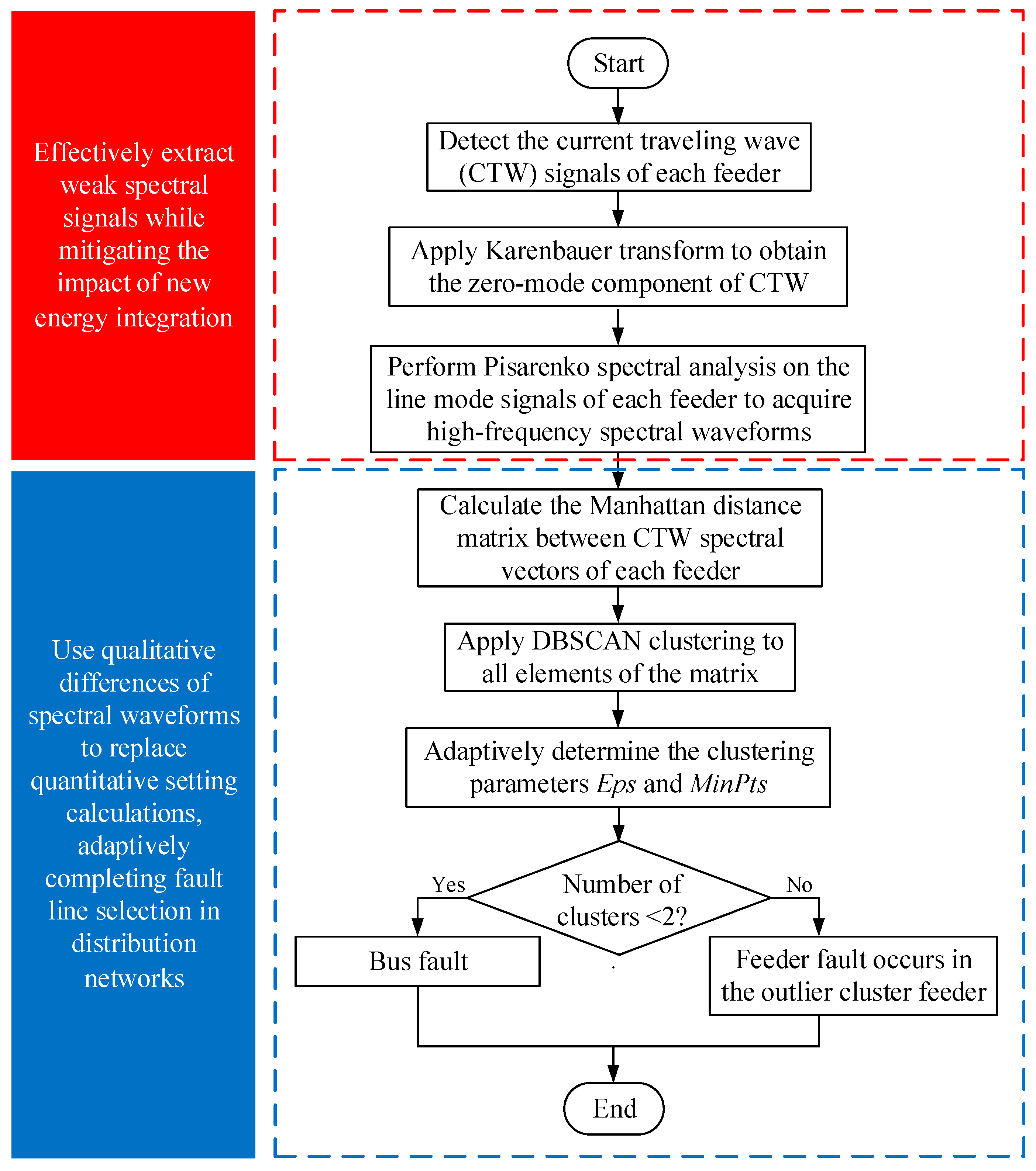
4.3. High Impedance Grounding Fault Line Detection Process of New Distribution Network
5. Simulation Analysis
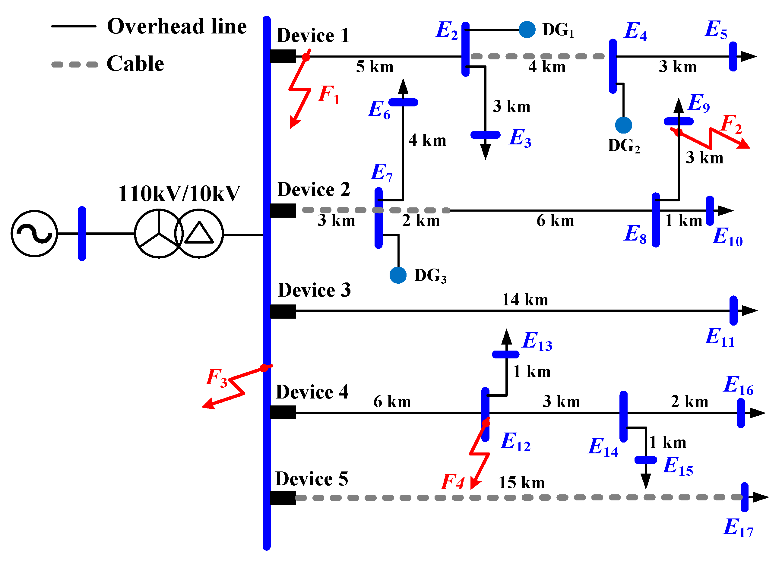
5.1. Simulation Model
5.2. Analysis of Line Detection Results
5.3. Adaptability Analysis of Line Detection Method
5.4. Comparative Analysis of Fault Line Selection Effect by Different Methods
5.5. Comparative Analysis of Line Detection Effect of Different Clustering Algorithms
6. Conclusions
Author Contributions
Funding
Data Availability Statement
Conflicts of Interest
References
- Meng, L.; Yang, X.; Zhu, J.; Wang, X.; Meng, X. Network Partition and Distributed Voltage Coordination Control Strategy of Active Distribution Network System Considering Photovoltaic Uncertainty. Appl. Energy 2024, 362, 122846. [Google Scholar] [CrossRef]
- Xiaotian, L.U.; Jinrui, T.; Xin, Y.I.N.; Yunhui, H.; Keliang, Z.; Chengqing, Y. Single-phase-to-ground Fault Section Location in New-type Distribution System Based on Multidimensional Time-frequency Distribution Characteristics. High Volt. Eng. 2025, 51, 903–914. [Google Scholar]
- Galvez, C.; Abur, A. Fault Location in Active Distribution Networks Containing Distributed Energy Resources (DERs). IEEE Trans. Power Deliv. 2021, 36, 3128–3139. [Google Scholar] [CrossRef]
- Chen, X.; Yuan, S.; Li, Z.; Ren, J.; Geng, S. A Novel Steady-State-Component-Based Current Differential Protection Scheme for Petal-Shaped Distribution Network with Inverter-Interfaced Distributed Generators. CSEE J. Power Energy Syst. 2022, 8, 1–11. [Google Scholar]
- Han, X.; Yan, X.; Ma, C.; Han, H. Fault Line Selection Method Based on Steady-State Zero-Sequence Voltage. In Proceedings of the International Conference on Energy Technology and Electrical Power (ETEP 2024), Guangzhou, China, 20–22 December 2024; SPIE: Bellingham, WA, USA; Volume 13566, pp. 384–389. [Google Scholar]
- Liang, Y.; Chen, H.; Ding, J.; Xu, Z.; Li, H.; Wang, G. Transient Analytical Method for Single-Ended Fault Location of AC Transmission Lines Considering Fuzzy Constraints of Fault Features. J. Mod. Power Syst. Clean Energy 2024, 10, 1–13. [Google Scholar]
- Tang, Y.; Chang, Y.; Tang, J.; Xu, B.; Ye, M.; Yang, H. A Novel Faulty Phase Selection Method for Single-Phase-to-Ground Fault in Distribution System Based on Transient Current Similarity Measurement. Energies 2021, 14, 4695. [Google Scholar] [CrossRef]
- Cheng, L.; Wang, T.; Wang, Y. A Novel Fault Location Method for Distribution Networks with Distributed Generations Based on the Time Matrix of Traveling-Waves. Prot. Control. Mod. Power Syst. 2022, 7, 46. [Google Scholar] [CrossRef]
- Liu, F.; Xie, L.; Yu, K.; Wang, Y.; Zeng, X.; Bi, L.; Liu, F.; Tang, X. A Novel Fault Location Method Based on Traveling Wave for Multi-Branch Distribution Network. Electr. Power Syst. Res. 2023, 224, 109753. [Google Scholar] [CrossRef]
- Wang, S.; Liu, C.; Wei, S. Research on Fault Line Selection Method Based on Steady State Variables. AIP Adv. 2024, 14, 075112. [Google Scholar] [CrossRef]
- Zhang, Y.; Shao, W. Fault Line Selection of Resonant Grounding System Using Transient Zero-Sequence Current Waveform Characteristics. In Proceedings of the 2022 International Conference on Computer Network, Electronic and Automation (ICCNEA), Xi’an, China, 23–25 September 2022; pp. 278–283. [Google Scholar]
- Guang, F.; Tinglong, G.; Lei, W.; Yongduan, X.U.E.; Xiaoyong, Y.U.; Bingyin, X.U. Grounding Fault Line Selection of Non-solidly Grounding System Based on Linearity of Current and Voltage Derivative. Power Syst. Technol. 2019, 45, 302–311. [Google Scholar]
- Wei, L.; Jia, W.; Jiao, Y. Single-Phase Fault Line Selection Scheme of a Distribution System Based on Fifth Harmonic and Admittance Asymmetry. Power Syst. Prot. Control. 2020, 48, 77–83. [Google Scholar]
- Li, Z.; Wan, J.; Wang, P.; Weng, H.; Li, Z. A Novel Fault Section Locating Method Based on Distance Matching Degree in Distribution Network. Prot. Control. Mod. Power Syst. 2021, 6, 1–11. [Google Scholar] [CrossRef]
- Xia, Y.; Li, Z.; Wang, S.; Sun, J.; Guo, X. Traveling Wave Inversion Method of Power Line Faults. Int. J. Electr. Power Energy Syst. 2023, 149, 109025. [Google Scholar] [CrossRef]
- Wang, Z.; Razzaghi, R.; Paolone, M.; Rachidi, F. Electromagnetic Time Reversal Similarity Characteristics and Its Application to Locating Faults in Power Networks. IEEE Trans. Power Deliv. 2020, 35, 1735–1748. [Google Scholar] [CrossRef]
- Yang, D.; Lu, B.; Lu, H. High-Resistance Grounding Fault Detection and Line Selection in Resonant Grounding Distribution Network. Electronics 2023, 12, 4066. [Google Scholar] [CrossRef]
- Deng, F.; Zu, Y.; Mao, Y.; Zeng, X.; Li, Z.; Tang, X.; Wang, Y. A Method for Distribution Network Line Selection and Fault Location Based on a Hierarchical Fault Monitoring and Control System. Int. J. Electr. Power Energy Syst. 2020, 123, 106061. [Google Scholar] [CrossRef]
- Tang, L.; Dong, X.; Luo, S.; Shi, S.; Wang, B. A New Differential Protection of Transmission Line Based on Equivalent Travelling Wave. IEEE Trans. Power Deliv. 2017, 32, 1359–1369. [Google Scholar] [CrossRef]
- Angrisani, L.; D’Apuzzo, M.; Grillo, D.; Pasquino, N.; Schiano Lo Moriello, R. A New Time-Domain Method for Frequency Measurement of Sinusoidal Signals in Critical Noise Conditions. Measurement 2014, 49, 368–381. [Google Scholar] [CrossRef]
- Li, J.; Wang, G.; Zeng, D.; Li, H. High-Impedance Ground Faulted Line-Section Location Method for a Resonant Grounding System Based on the Zero-Sequence Current’s Declining Periodic Component. Int. J. Electr. Power Energy Syst. 2020, 119, 105910. [Google Scholar] [CrossRef]
- Jiang, B.; Dong, X.; Shi, S. A Method of Single Phase to Ground Fault Feeder Selection Based on Single Phase Current Traveling Wave for Distribution Lines. Proc. CSEE 2014, 34, 6216–6227. [Google Scholar]
- Zichang, L.; Yadong, L.; Yingjie, Y.; Peng, W.; Xiuchen, J. An Identification Method for Asymmetric Faults With Line Breaks Based on Low-Voltage Side Data in Distribution Networks. IEEE Trans. Power Deliv. 2021, 36, 3629–3639. [Google Scholar] [CrossRef]
- Yalçın, F.; Yıldırım, Y. A Study of Symmetrical and Unsymmetrical Short Circuit Fault Analyses in Power Systems. Sak. Univ. J. Sci. 2019, 23, 879–895. [Google Scholar] [CrossRef]
- Wang, W.; Gao, X.; Fan, B.; Zeng, X.; Yao, G. Faulty Phase Detection Method Under Single-Line-to-Ground Fault Considering Distributed Parameters Asymmetry and Line Impedance in Distribution Networks. IEEE Trans. Power Deliv. 2022, 37, 1513–1522. [Google Scholar] [CrossRef]
- Guo, M.-F.; Cai, W.-Q.; Zheng, Z.-Y.; Wang, H. Fault Phase Selection Method Based on Single-Phase Flexible Arc Suppression Device for Asymmetric Distribution Networks. IEEE Trans. Power Deliv. 2022, 37, 4548–4558. [Google Scholar] [CrossRef]
- Jankovski, M.; Popov, M.; Godefrooi, J.; Parabirsing, E.; Wierenga, E.; Lekić, A. Novel Busbar Protection Scheme for Impedance-Earthed Distribution Networks. Electr. Power Syst. Res. 2023, 223, 109569. [Google Scholar] [CrossRef]
- Mousaviyan, I.; Seifossadat, S.G.; Saniei, M. Traveling Wave-Based Algorithm for Fault Detection, Classification, and Location in STATCOM-Compensated Parallel Transmission Lines. Electr. Power Syst. Res. 2022, 210, 108118. [Google Scholar] [CrossRef]
- Kersting, W.H. Distribution System Modeling and Analysis. In Electric Power Generation, Transmission, and Distribution; CRC Press: Boca Raton, FL, USA, 2012; ISBN 978-1-315-22242-4. [Google Scholar]
- Wang, Y.; Feng, C.; Liu, J.; Dong, X.; Yuan, J.; Jiao, Z. Faulty Line Detection for Cross-line Same-phase Successive Ground Faults in Distribution Network Based on Transient Characteristics. IET Gener. Transm. Distrib. 2024, 18, 1624–1640. [Google Scholar] [CrossRef]
- Ni, Y.; Zeng, X.; Liu, Z.; Yu, K.; Xu, P.; Wang, Z.; Zhuo, C.; Huang, Y. Faulty Feeder Detection of Single Phase-to-Ground Fault for Distribution Networks Based on Improved K-Means Power Angle Clustering Analysis. Int. J. Electr. Power Energy Syst. 2022, 142, 108252. [Google Scholar] [CrossRef]
- Wenjun, G.; Heng, W.; Ying, Z. Fault Line Selection of Small Current Grounding System Research Based on Zero Sequence Circuit Current Phase. J. Phys. Conf. Ser. 2024, 2872, 012049. [Google Scholar] [CrossRef]
- Xie, L.; Luo, L.; Ma, J.; Li, Y.; Zhang, M.; Zeng, X.; Cao, Y. A Novel Fault Location Method for Hybrid Lines Based on Traveling Wave. Int. J. Electr. Power Energy Syst. 2022, 141, 108102. [Google Scholar] [CrossRef]


| Line Type | Impedance/(Ω/km) | Inductance/(mH/km) | Capacitance/(μF/km) | |||
|---|---|---|---|---|---|---|
| Positive Sequence | Zero Sequence | Positive Sequence | Zero Sequence | Positive Sequence | Zero Sequence | |
| Overhead Line | 0.170 | 0.230 | 1.210 | 5.475 | 0.009 | 0.006 |
| Cable | 0.270 | 2.700 | 1.019 | 0.255 | 0.339 | 0.280 |
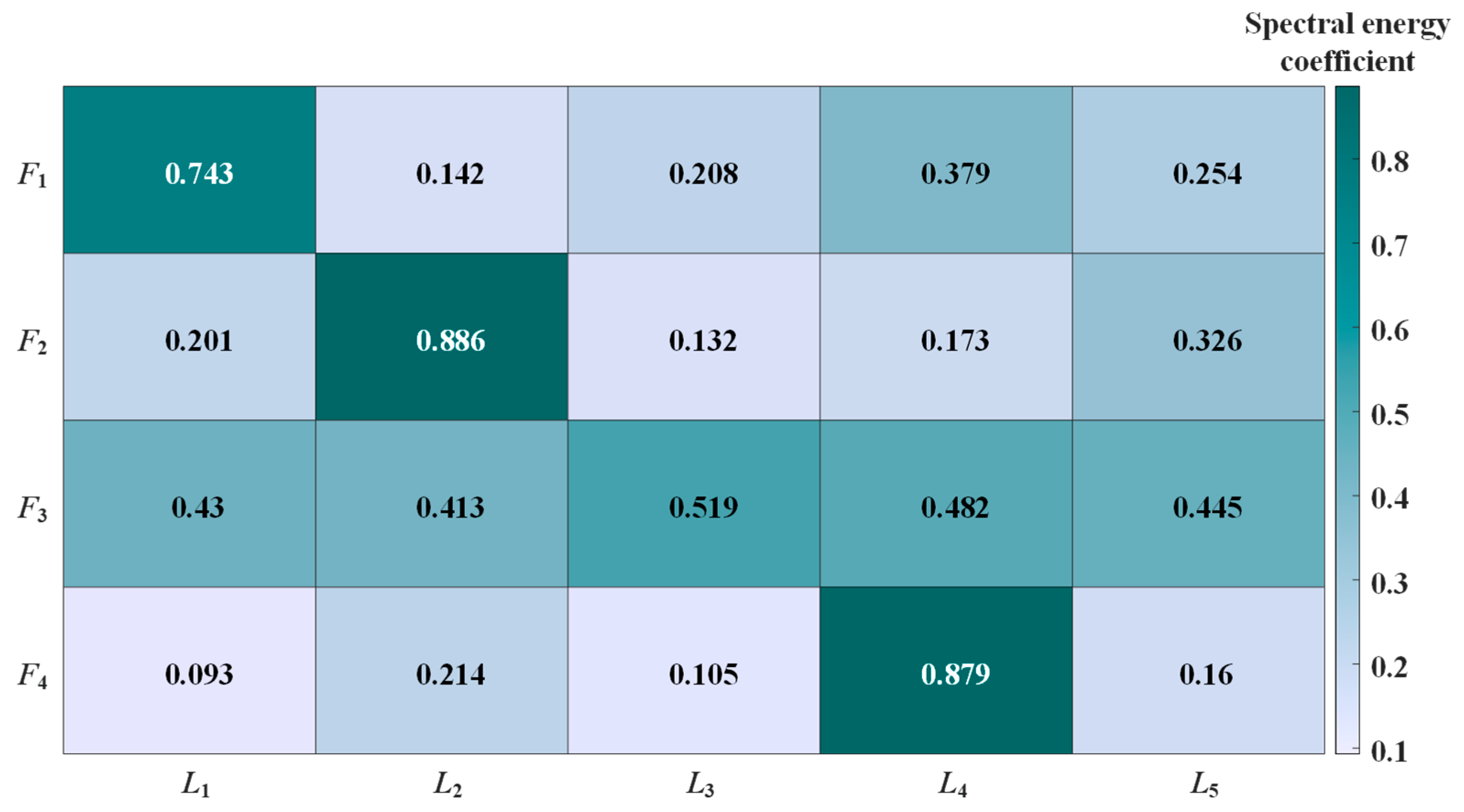
| Fault Location | Spectral Energy Coefficient [p1, p2, p3, p4, p5] | Cluster Label | Fault Line Identification Result |
|---|---|---|---|
| F1 | [0.743, 0.142, 0.208, 0.379, 0.254] | [2 1 1 1 1] | L1 |
| F2 | [0.201, 0.886, 0.132, 0.173, 0.326] | [1 2 1 1 1] | L2 |
| F3 | [0.430, 0.413, 0.519, 0.482, 0.445] | [1 1 1 1 1] | Bus |
| F4 | [0.093, 0.214, 0.105, 0.879, 0.160] | [1 1 1 2 1] | L4 |
| Fault Location | Fault Esistance/kΩ | Fault Type | Spectral Energy Coefficient [p1, p2, p3, p4, p5] | Cluster Label | Fault Line Identification Result |
|---|---|---|---|---|---|
| F1 | 5 | Phase-A grounding | [0.743, 0.142, 0.208, 0.379, 0.254] | [2 1 1 1 1] | L1 |
| 8 | Phase-B grounding | [0.699, 0.145, 0.193, 0.388, 0.266] | [2 1 1 1 1] | L1 | |
| 10 | Phase-C grounding | [0.718, 0.140, 0.214, 0.357, 0.258] | [2 1 1 1 1] | L1 | |
| F2 | 5 | Phase-A grounding | [0.201, 0.886, 0.132, 0.173, 0.326] | [1 2 1 1 1] | L2 |
| 8 | Phase-B grounding | [0.209, 0.865, 0.124, 0.162, 0.338] | [1 2 1 1 1] | L2 | |
| 10 | Phase-C grounding | [0.201, 0.871, 0.139, 0.183, 0.356] | [1 2 1 1 1] | L2 | |
| F3 | 5 | Phase-A grounding | [0.430, 0.413, 0.519, 0.482, 0.445] | [1 1 1 1 1] | Bus |
| 8 | Phase-B grounding | [0.457, 0.405, 0.503, 0.500, 0.436] | [1 1 1 1 1] | Bus | |
| 10 | Phase-C grounding | [0.441, 0.422, 0.510, 0.492, 0.455] | [1 1 1 1 1] | Bus | |
| F4 | 5 | Phase-A grounding | [0.093, 0.214, 0.105, 0.879, 0.160] | [1 1 1 2 1] | L4 |
| 8 | Phase-B grounding | [0.095, 0.224, 0.085, 0.825, 0.156] | [1 1 1 2 1] | L4 | |
| 10 | Phase-C grounding | [0.106, 0.217, 0.101, 0.903, 0.152] | [1 1 1 2 1] | L4 |
| New Energy Types | DG3 Capacity/dB | Noise/dB | Spectral Energy Coefficient [p1, p2, p3, p4, p5] | Cluster Label | Fault Line Identification Result |
|---|---|---|---|---|---|
| Fuel Cell | 0.1 | 20 | [0.209, 0.865, 0.124, 0.162, 0.338] | [1 2 1 1 1] | L2 |
| 8 | 30 | [0.203, 0.825, 0.108, 0.156, 0.338] | [1 2 1 1 1] | L2 | |
| 15 | 40 | [0.194, 0.818, 0.127, 0.162, 0.340] | [1 2 1 1 1] | L2 | |
| Photovoltaic Cell | 0.1 | 20 | [0.209, 0.865, 0.124, 0.162, 0.338] | [1 2 1 1 1] | L2 |
| 8 | 30 | [0.241, 0.844, 0.131, 0.191, 0.368] | [1 2 1 1 1] | L2 | |
| 15 | 40 | [0.193, 0.858, 0.125, 0.187, 0.340] | [1 2 1 1 1] | L2 |
| Method | Percentage Success | Advantage | Disadvantage |
|---|---|---|---|
| Steady-state component method | 80% | Not affected by transition resistance and fault type | Weak steady-state component characteristics; low reliability of detection signal |
| Transient-state component method [32] | 85% | More obvious signal; certain improvement in line selection accuracy | Fault line determination is easily affected by system operation mode and parameter changes |
| Traditional traveling-wave method [33] | 88% | Not affected by transition resistance, CT saturation, etc. | Inadequate utilization of frequency-domain characteristics; limited effect in complex scenarios |
| Proposed method | 97.5% | Not affected by weak fault signals in short data windows caused by renewable energy integration; applicable to various neutral-grounding methods and renewable energy operation scenarios; uses qualitative dissimilarity of spectral waveform characteristics to replace quantitative threshold calculation, solving threshold-setting challenges and achieving high sensitivity and reliability | No obvious disadvantage found yet |
| Clustering Algorithm | Fault Line Detection Accuracy/% | Silhouette Coefficient |
|---|---|---|
| K-means clustering | 86.7 | 0.70 |
| Fuzzy c-means clustering | 85.4 | 0.73 |
| Hierarchical clustering | 82.3 | 0.69 |
| Spectral clustering | 82.5 | 0.62 |
| DBSCAN clustering | 97.5 | 0.85 |
Disclaimer/Publisher’s Note: The statements, opinions and data contained in all publications are solely those of the individual author(s) and contributor(s) and not of MDPI and/or the editor(s). MDPI and/or the editor(s) disclaim responsibility for any injury to people or property resulting from any ideas, methods, instructions or products referred to in the content. |
© 2025 by the authors. Licensee MDPI, Basel, Switzerland. This article is an open access article distributed under the terms and conditions of the Creative Commons Attribution (CC BY) license (https://creativecommons.org/licenses/by/4.0/).
Share and Cite
Xiao, M.; Zeng, J.; Zhou, Z.; Zhang, Q.; Deng, L.; Peng, F. High Impedance Fault Line Detection Based on Current Traveling Wave Spectrum Symmetry Driving for New Distribution Network. Symmetry 2025, 17, 775. https://doi.org/10.3390/sym17050775
Xiao M, Zeng J, Zhou Z, Zhang Q, Deng L, Peng F. High Impedance Fault Line Detection Based on Current Traveling Wave Spectrum Symmetry Driving for New Distribution Network. Symmetry. 2025; 17(5):775. https://doi.org/10.3390/sym17050775
Chicago/Turabian StyleXiao, Maner, Jupeng Zeng, Zehua Zhou, Qiming Zhang, Li Deng, and Feiyu Peng. 2025. "High Impedance Fault Line Detection Based on Current Traveling Wave Spectrum Symmetry Driving for New Distribution Network" Symmetry 17, no. 5: 775. https://doi.org/10.3390/sym17050775
APA StyleXiao, M., Zeng, J., Zhou, Z., Zhang, Q., Deng, L., & Peng, F. (2025). High Impedance Fault Line Detection Based on Current Traveling Wave Spectrum Symmetry Driving for New Distribution Network. Symmetry, 17(5), 775. https://doi.org/10.3390/sym17050775