A Novel Approach in 3D Model Reconstruction from Engineering Drawings Based on Symmetric Adjacency Matrices Using DXF Files and Genetic Algorithm

Abstract

The application of CAD/CAM technologies in modern production has revolutionized manufacturing processes, leading to significant improvements in precision, efficiency, and flexibility. These technologies enable the design and manufacturing of complex geometries with high accuracy, reducing errors and material waste. CAD/CAM integration streamlines workflows, enhances productivity, and facilitates rapid prototyping, accelerating the time-to-market for new products. Additionally, it supports customization and scalability in production, allowing for cost-effective small-batch and large-scale manufacturing. Without a 3D model of the product, it is not possible to use the advantages of applying advanced CAD/CAM technologies. Recognizing 3D models from engineering drawings is essential for modern production, especially for outsourcing companies in fluctuating market conditions, where the production process is organized with 2D workshop drawings on paper. This paper proposes a novel methodology for reconstructing 3D models from 2D engineering drawings, specifically those in DXF file format, leveraging a genetic algorithm. A core component of this approach is the representation of the 2D drawing as a symmetric adjacency matrix. This matrix serves as the foundational data structure for the genetic algorithm, enabling the evolutionary process to effectively optimize the 3D reconstruction. The experimental evaluation, conducted on multiple engineering drawing test cases (including both polyhedral and cylindrical geometries), demonstrated consistent convergence of the proposed GA-based method toward topologically valid and geometrically accurate 3D wireframe models. The approach achieved successful reconstruction in all cases, with fitness scores ranging from 1.1 to 112.2 depending on model complexity, and average execution times from 2 to 100 s. These results confirm the method’s robustness, scalability, and applicability in real-world CAD environments, while establishing a new direction for topology-driven 3D reconstruction using evolutionary computation.

1. Introduction

The integration of computer-aided design and computer-aided manufacturing (CAD/CAM) technologies has profoundly transformed modern manufacturing by enabling rapid prototyping, design precision, and flexible production. However, in many industrial environments, particularly those relying on legacy documentation, two-dimensional (2D) workshop drawings remain the predominant format for technical communication. These drawings are often the only documentation available, especially in subcontracting or archival scenarios, making the automatic reconstruction of three-dimensional (3D) models from 2D sources a critical challenge.

The reconstruction of 3D models from 2D technical drawings is a key problem in CAD, reverse engineering, and model understanding. Orthographic projections, as standardized 2D representations, encode critical geometric and topological information of an object, yet lack depth and perspective, making the reconstruction process inherently underdetermined and often ambiguous.

Despite decades of research, the fully automated reconstruction of 3D models from 2D orthographic drawings remains a technically demanding problem. The majority of existing approaches are either limited to specific object categories (e.g., polyhedral shapes), require supervised learning with annotated datasets, or rely heavily on manually defined features and heuristics. One critical limitation is the absence of topological data in standard formats such as Drawing Exchange Format (DXF), which only contain isolated geometric entities (lines, arcs, circles) without information on how these entities are connected across views. This is particularly evident in the case of the DXF. Developed by Autodesk, DXF is an open, CAD-native file format originally created to enable interoperability between different CAD systems. In a DXF file, each geometric entity is represented by a structured ASCII or binary record, which facilitates programmatic extraction of coordinates and primitive types but does not include explicit topological connectivity.

Moreover, many methods do not generalize well to complex industrial parts that include curved surfaces, intersecting features, or non-standard projection layouts. Computational complexity is another barrier, as approaches based on exhaustive geometric matching or volumetric reconstruction often become infeasible for drawings with a high number of elements. Consequently, there is a clear need for reconstruction methods that can operate without prior knowledge of shape classes, while remaining computationally tractable and tolerant to incomplete or ambiguous input data.

Automated 3D reconstruction from 2D orthographic projections has become increasingly important due to its role in streamlining digital manufacturing workflows. Since 3D models serve as the foundation for CAM (such as AutoCAD Mechanical v24.0) software and the generation of CNC programs, their availability is essential for modern production systems. Manual reconstruction is time-consuming, error-prone, and incompatible with the demands of scalable, automated manufacturing environments.

Recent studies have attempted to address these limitations through machine learning models, rule-based extraction, and graph-based interpretations. For example, Furferi et al. [1] employed a set of geometric rules for feature recognition, while Zhang et al. [2] proposed a method based on shape matching and solid feature extraction. However, these approaches typically depend on either specific geometric constraints or extensive domain knowledge, which limits their flexibility. CNN-based techniques [3,4] have shown promise in object classification tasks but are not easily adaptable to wireframe reconstruction without labeled training datasets.

Furthermore, although some researchers have explored the use of genetic algorithms (GA) for reconstruction tasks [5], these efforts are often restricted to prismatic objects or simplified scenarios with predefined projections. To the best of our knowledge, no existing study has formulated the reconstruction task using a symmetric topological representation that abstracts the geometry into a generalized graph structure. This gap highlights the need for a new approach that combines topological abstraction and evolutionary optimization to address the limitations of current methods in terms of generality, scalability, and independence from geometric priors.

The primary purpose of this study is to develop a robust and generalizable methodology for reconstructing 3D wireframe models from 2D orthographic engineering drawings in DXF format. Unlike existing methods that rely on geometry-specific rules or extensive training datasets, our approach seeks to abstract the reconstruction process by modeling the structural relationships within the drawing. This enables the proposed method to function independently of specific shape types and to be applicable to a broad range of industrial components, including those with curved or hybrid geometries.

To address these challenges, this paper proposes a novel method that integrates geometric reasoning with a topological representation based on symmetric adjacency matrices. This representation compactly encodes the relationships between vertices and edges, supporting efficient detection of geometric consistencies and inconsistencies across projections. The proposed method extracts geometric entities directly from DXF files and constructs a connectivity matrix that forms the basis for identifying spatial relations. A GA is then employed to search the solution space for a plausible 3D reconstruction that satisfies geometric constraints while aligning projections from multiple views. This hybrid strategy enhances automation and robustness, particularly in reconstructing wireframe models from standard 2D technical drawings.

The proposed approach is expected to achieve accurate and consistent reconstruction of 3D wireframe models from 2D technical drawings, even in cases where traditional methods fail due to geometric ambiguity or incomplete data. Through extensive testing on real-world engineering examples—including both polyhedral and cylindrical components—the method is designed to demonstrate strong generalization capabilities, low computational overhead, and high structural fidelity. These outcomes would confirm the practical potential of the approach for integration into CAD/CAM workflows and digital twin environments.

The remainder of this paper is organized as follows. Section 2 reviews the background and related work in 3D reconstruction from 2D drawings, focusing on existing methodologies and identifying research gaps. Section 3 presents the theoretical model, outlining the assumptions, mathematical formulation, and the complete workflow for wireframe reconstruction using symmetric adjacency matrices. Section 4 introduces the genetic algorithm developed for optimization, including chromosome representation, fitness evaluation, and evolutionary operators. Section 5 discusses the experimental setup and presents results obtained on several real-world test cases, including polyhedral and cylindrical geometries. Section 6 concludes the paper with a summary of findings, identified limitations, and future research directions.

2. Background and Related Work

The reconstruction of 3D models from 2D technical drawings has been explored since the 1970s, primarily through two fundamental approaches: Boundary Representation (B-Rep) and Constructive Solid Geometry (CSG). B-Rep describes objects by their boundaries (vertices, edges, and surfaces), while CSG relies on Boolean operations over basic geometric primitives. The first known algorithm for generating 3D models from orthographic projections was introduced in 1973 [2] and later formalized in subsequent works [3,4]. These early methods mainly focused on polyhedral object reconstruction, with a more efficient algorithm proposed in [5].

Previous studies on 3D model reconstruction from 2D drawings have explored a range of methodologies, including rule-based systems, graph-based representations, and evolutionary computation. Zhang et al. [2] classify existing methods into three main groups: wireframe reconstruction, direct solid reconstruction, and machine learning-based methods. This classification can be extended to include metaheuristic approaches such as GAs, which, despite their potential, remain relatively underexplored. A comprehensive review of modern methods is provided in [2].

Within the wireframe domain, Furferi et al. [1] developed a MATLAB v7. 10 algorithm that utilizes vector drawings and vertex connectivity to construct 3D models. The authors in [6] applied fuzzy logic to analyze surface connectivity, while [7] addressed the construction of conic curves using Bézier interpolation. However, most methods struggle with curved edges and complex shapes. A decision tree approach is used in [8] to recognize surfaces from all three projections, though the algorithm is complex due to multiple parallel analyses.

Further developments include [9,10,11,12], which introduce a hybrid model linking vertices, edges, and surfaces, later converted into B-Rep. Although informative, this method requires high computational resources due to surface relation identification in each view. Varley [12] applied shortest path algorithms on graphs to detect loops corresponding to surfaces. Others, such as [13,14], rely on extrusion and knowledge bases but are limited to simple forms and predefined geometries.

Machine learning approaches—particularly convolutional and transformer neural networks—are becoming more prominent, yet a functional model for direct 3D reconstruction from 2D drawings is still lacking [9], and thus this work does not explore that domain further.

Among metaheuristic strategies, GAs show promise. Chen and Feng [15] were the first to apply GAs for reconstructing 3D models from imprecise 2D contours. Similar concepts have been explored in [16,17,18], although these are largely limited to prismatic shapes and do not handle more complex surfaces.

Based on the literature, three main challenges can be identified: high computational complexity, limited applicability to drawings with mixed geometries, and underutilization of genetic algorithms. This paper introduces a novel method based on symmetric connectivity matrices, which efficiently encodes the topology of 2D entities extracted from DXF files and serves as the foundation for GA-based optimization. Our approach enables wireframe model reconstruction through graph-based traversal, independent of shape complexity, including lines, arcs, and curves.

Unlike existing GA approaches that operate on contours or raster images, our method uses a graph-based representation with clearly defined topology. To the best of our knowledge, this is the first work to formulate wireframe reconstruction as a graph optimization problem addressed via evolutionary algorithms. The method demonstrates good performance and opens promising directions for further research. The proposed method not only enhances the efficiency of shape reconstruction but also emphasizes the inherent symmetry in structural representations of engineering geometries.

3. Model Elements and Workflow for 3D Model Reconstruction from 2D Engineering Drawings

3.1. Initial Hypotheses and Assumptions

This paper hypothesizes that representing 2D orthographic projections using symmetric adjacency matrices enables efficient, scalable, and accurate reconstruction of 3D wireframe models through evolutionary optimization. The central assumption is that the topological and geometric relationships inherent in 2D technical drawings can be compactly encoded in symmetric matrices and interpreted as graph structures, forming a consistent foundation for reconstructing 3D geometry.

The main contributions of this paper are:

• A novel representation of 2D engineering drawings using symmetric adjacency matrices.
• A mathematical model that formalizes the 3D wireframe reconstruction problem as a binary integer optimization task.
• Development and implementation of a customized genetic algorithm for solving this optimization problem
• Experimental validation across both polyhedral and cylindrical geometries, demonstrating the method’s generality and robustness, including cases with curved edges and varying levels of drawing complexity.

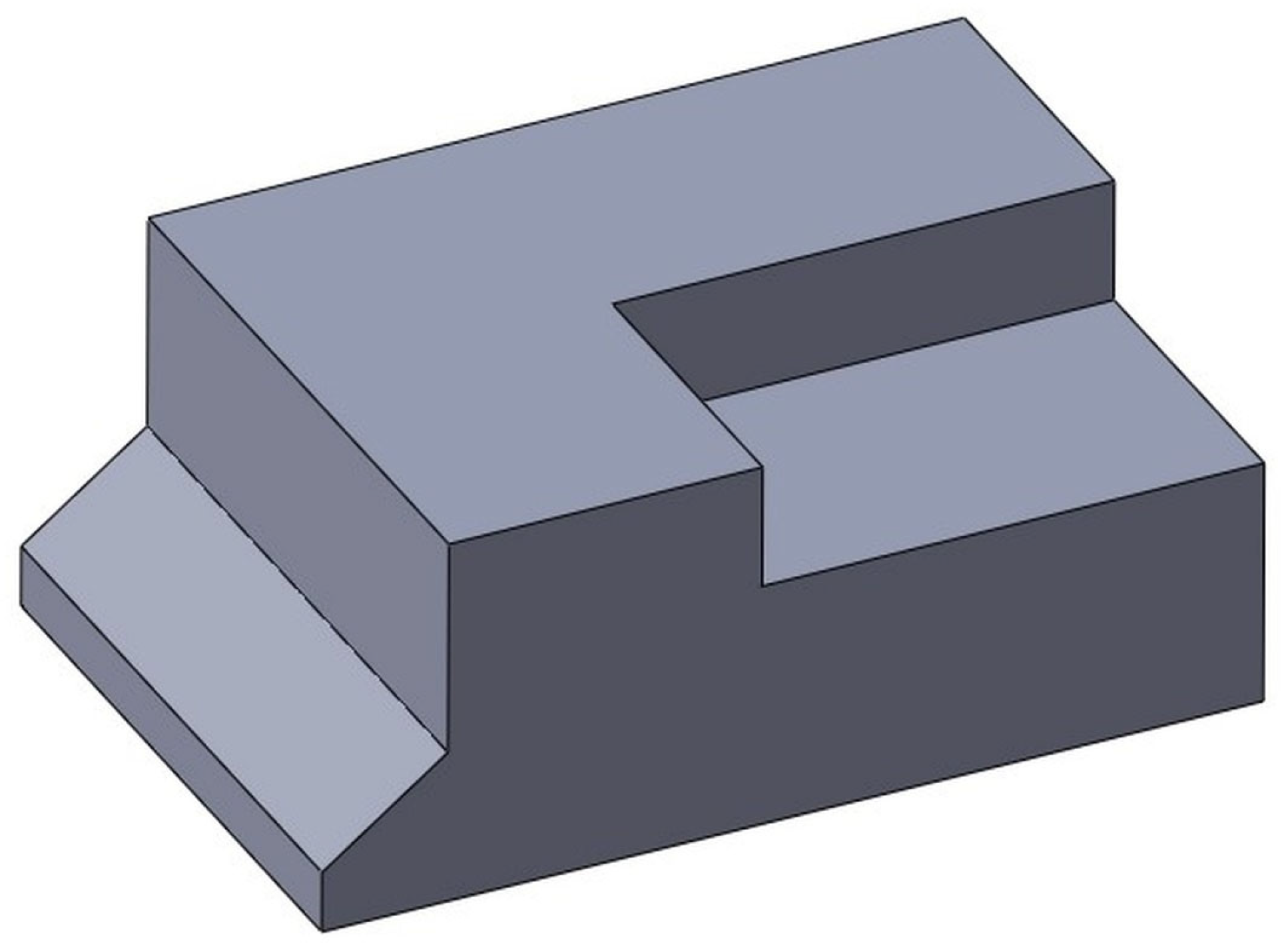
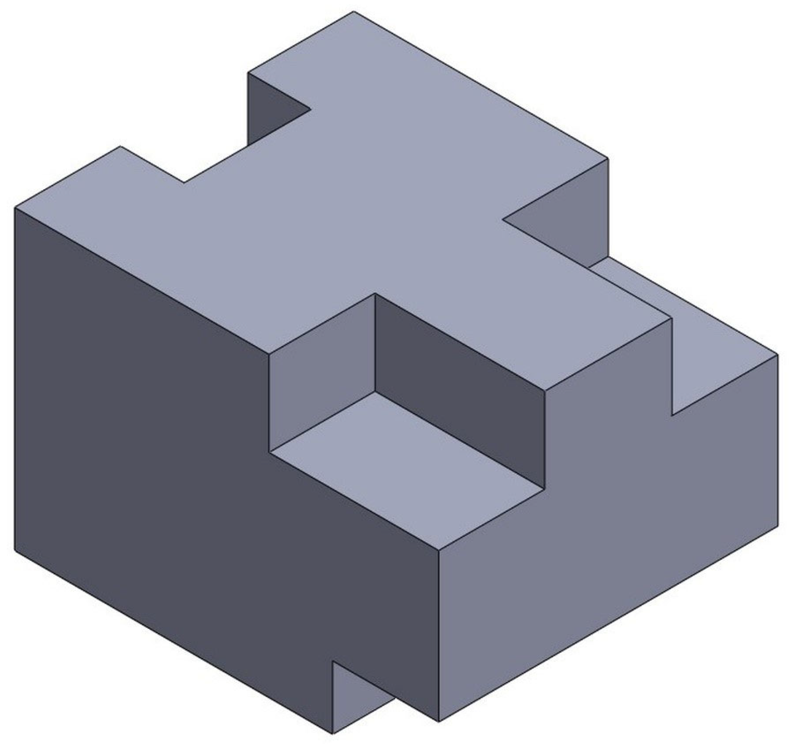
Figure 1 shows a 3D model of a typical industrial machine part, designed in one of the software packages.

For drawing creation, including the method of marking individual components of the drawing, certain conventions have been adopted over the past decades and regulated by appropriate standards [19]. The goal of adopting these conventions is to ensure that drawings provide unambiguous instructions for the manufacture of the depicted parts. These standards, whether international ISO standards or national standards, are integrated into commercial software packages and offer multiple options for representing individual elements of machine parts in technical or workshop drawings. These options provide designers with some freedom when creating workshop drawings, making it practically impossible to incorporate all possibilities into an algorithm for identifying geometric information. Therefore, this research is based on the following assumptions:

It is assumed that the 2D workshop drawing is complete and contains three orthographic projections made according to ISO-E or European projection layout: front view, top view, and left view, as shown in Figure 2.

It is assumed that the 2D workshop drawing contains all the necessary information that clearly and unambiguously defines the shape of the machine part. Sections, details, partial views, etc., are not considered, meaning all edges, vertices, and hidden lines are shown in the corresponding projections (Figure 2).

The dimensions of the 3D model can be directly obtained from the vertex coordinates, assuming they can be corrected with an appropriate scaling factor. For simplicity, this research assumes that the orthographic projections are created at a scale of 1:1.

It is assumed that all three orthographic projections are created in accordance with the dimensional and geometric tolerances previously embedded in the 3D model.

DXF files, due to their binary or ASCII format, offer a significant advantage in entity recognition tasks, as highlighted in [20,21]. This format simplifies the identification of geometric entities such as lines, circles, points, and polylines within engineering drawings. When an object is provided with three projections in the DXF format, identifying the individual components (such as lines, circles, etc.) is a relatively straightforward process. However, the DXF format lacks topological data, meaning the file contains no logical sequence for the entities and no explicit information about their connectivity. In simpler terms, details about the spatial arrangement of projections and the edges associated with them are absent. Due to this limitation, a method to separate the drawing into three distinct views is required before proceeding with further analysis [6].

These assumptions simplify the input data for the process of the identification and conversion of geometric information, enabling its practical implementation. Without these assumptions, the process of identifying and recognizing geometric information would significantly exceed the scope of this research.

3.2. Workflow of 3D Reconstruction Process

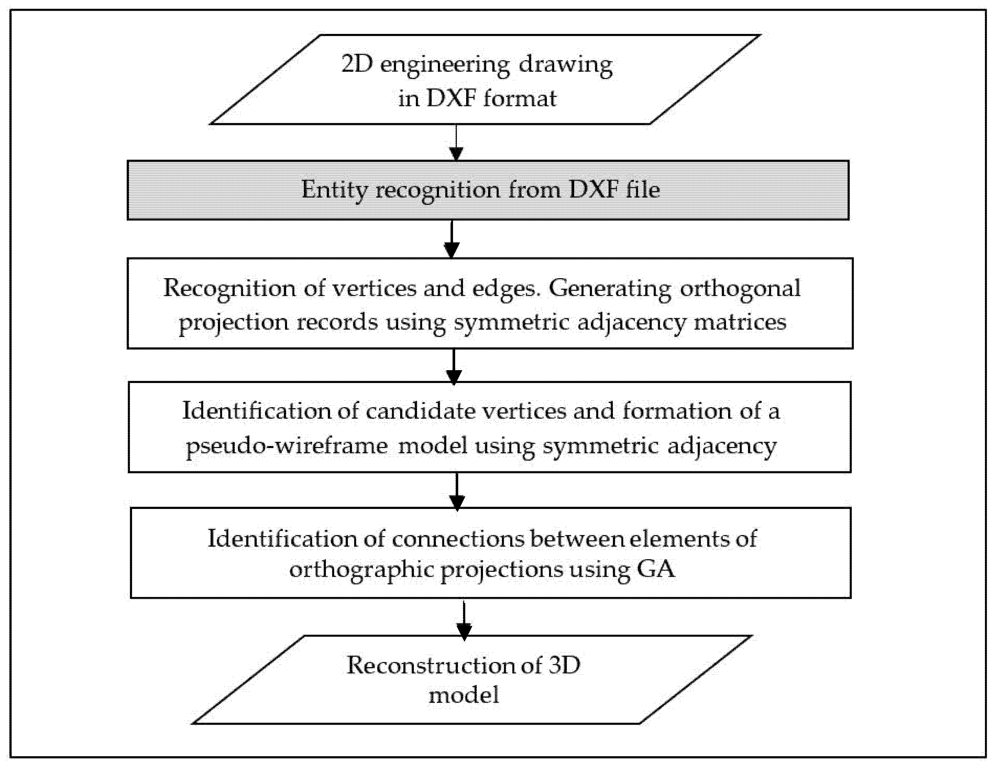
The flowchart presented in Figure 3 outlines the overall workflow of the proposed methodology, beginning with the parsing of DXF projections and culminating in the reconstruction process based on a GA. Each element of the flowchart corresponds to a specific sub-procedure, the details of which are elaborated in the subsequent sections. This modular structure ensures clarity and reproducibility, reflecting the systematic integration of geometric data processing and evolutionary optimization.

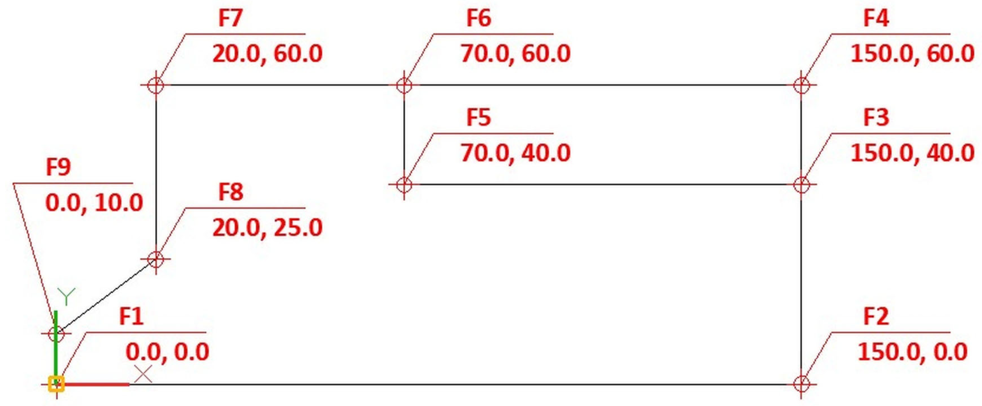
The orthographic projections shown in Figure 4, which are analogous to the example found in [16] consist of different flat geometric shapes. These shapes can be lines, circular arcs and circles. Those geometric shapes represent entities that form contours as shown in Figure 4. Also, it should be noted that entities are defined by their starting and ending points and some other characteristics that depend on the type of the entity.

In the example shown in Figure 4, which represents the front view of the part shown in Figure 1, there are a total of 9 points that form line entities. A line is an entity determined with the starting point (X₁, Y₁) and the ending point (X₂, Y₂), i.e., the coordinates of the starting and ending points in the Cartesian coordinate system.

In addition to line entities, there are also entity circle, determined by the coordinate of the center (X, Y) in the Cartesian coordinate system, and the radius R and an Arc or circular arc, determined by the coordinate of the center (X, Y) in the Cartesian coordinate system and the radius R, as well as the initial and final angle of the circular arc expressed in degrees.

Recognizing lines, circles, points, and polylines is fundamental to automated 3D model recognition, as they define surface boundaries. While entities recognition and positioning in DXF files are relatively simple and well documented in [16], our research addresses the more complex challenge of automatically establishing topological relationships between vertices and edges. The following presents the structured pseudocode for the extraction of line entities from the entities section of a DXF file. A similar approach is used for processing circular arcs and other entity types (Algorithm 1).

The procedure is organized into five key stages:

• File selection: User selects a DXF file from disk.
• Data initialization: The file is loaded and the ENTITIES section is located.
• Parsing logic: LINE entities are scanned and decomposed into vertex coordinate pairs.
• Edge creation: Edges are constructed by linking each vertex pair.
• Post-processing: Duplicate vertices are removed and the final vertex and edge arrays are produced.

Algorithm 1 Extraction of line entities and graph construction from a DXF file.

PROCEDURE ExtractLineEntities   INPUT: FilePath (string)–dxf file path   OUTPUT: VertexList (list of unique vertices), EdgeList (list of edges)   // 1. File selection   Open DXF file at FilePath   IF file cannot be opened THEN     RETURN error   // 2. Data initialization   Locate “ENTITIES” section in file   IF “ENTITIES” section not found THEN     RETURN error   Initialize empty list RawVertices   Initialize empty list EdgeList   // 3. Parsing logic   FOR each entity in “ENTITIES” section DO     IF entity type is “LINE” THEN         Read start point (X1, Y1)         Read end point (X2, Y2)     // 4. Edge creation         Add (X1, Y1) to RawVertices         Add (X2, Y2) to RawVertices         Add edge: ( (X1, Y1), (X2, Y2) ) to EdgeList     END IF   END FOR   // 5. Post-processing   VertexList ← Remove duplicate points from RawVertices   FOR each edge in EdgeList DO     Replace (X1, Y1) and (X2, Y2) with corresponding indices in VertexList   END FOR   RETURN VertexList, EdgeList END PROCEDURE

3.3. Creating Orthographic Projection Matrices

This section expands on how edges are formed from vertices based on their coordinates, and how this relationship is mathematically represented to construct the adjacency matrix AdjA for the front view (Figure 4).

Definition 1.

Let:

$P=\left\{p_1,p_2,\dots ,p_3\right\}$: A set VA of $n$ vertices in the front orthographic projection. Each vertex is represented as: $p_i=\left\{x_i,y_j\right\},i,j\in \left\{1,2,\dots ,n\right\}$

$E=\left\{e_1,e_2,\dots ,e_3\right\}$: A set EA of $m$ edges, where each edge $e_k$ connects two vertices $p_i$ and $p_j$. Each edge is represented as: $e_k=\left\{p_i,p_j\right\},i,j\in \left\{1,2,\dots ,n\right\},i\ne j$

Each entity is defined by a start point $\left(x_s, y_s\right)$, and an endpoint $\left(x_k, y_k\right)$.

Edge is defined by start and end points.

$$p_i=\left(x_s,y_s\right),\hspace{1em}{p}_j=\left(x_e,y_e\right)\hspace{1em}{e}_k=\left(p_i,p_j\right).$$

If the start or end point does not exactly match a vertex in P, a proximity threshold  ϵ > 0  to account for numerical inaccuracies can be applied: $p_i-(x_s,y_s)\Vert \le ϵ \mathit{and} \Vert p_j-(x_e,y_e)\Vert \le ϵ$

The adjacency matrix is defined as:

$$AdjA\in {\mathbb{R}}^{n\times n},\hspace{1em}AdjA\left[i,j\right]=\left\{\begin{array}{cc}1,& \mathrm{if} \left(p_i,p_j\right)\in E\\ 0,& \mathrm{otherwise}.\end{array}\right.$$

where indicates that an edge exists between vertices. It is important to notice that orthogonal projection can be represented as an undirected graph [16] and then the matrix  $AdjA$ is symmetric: 

$$AdjA\left[i,j\right]=AdjA\left[j,i\right],\forall i,j.$$

Diagonal elements $AdjA\left[i,i\right]=0$-no self-loops are considered as: $AdjA\left[i,i\right]=0,\forall i.$

The adoption of symmetric adjacency matrices is driven by their capacity to compactly encode topological relationships among vertices in a standardized and computationally efficient format. In contrast to edge lists or conventional graph-based representations, symmetric matrices inherently minimize redundancy—owing to their structural symmetry—and support efficient matrix operations, such as the computation of the Frobenius norm, which plays a critical role in the iterative optimization process governed by GA. Furthermore, this representation naturally corresponds to the undirected nature of edge relationships in engineering drawings, thereby preserving consistent connectivity across multiple orthographic projections. By abstracting geometric entities into binary topological relations, the proposed approach achieves a high level of generality, effectively handling both linear and curved elements without introducing additional algorithmic complexity.

The preceding definitions lay the groundwork for constructing the adjacency matrix representing the orthogonal projection. The construction of an adjacency matrix is a simple algorithm and for verifying the consistency of the matrix two important rules should be checked as follows:

• Edge count: The total number of edges, i.e., 1’s in $AdjA$ (excluding diagonal elements) should be equal 2m for m edges: ${\sum }_{i,j}Adj{A}_{ij}-{\sum }_{i}Adj{A}_{ii}=2m$;
• Symmetry: For undirected graph: $AdjA=Adj{A}^T$.

However, there is one difference in this study that is very important for the research presented.

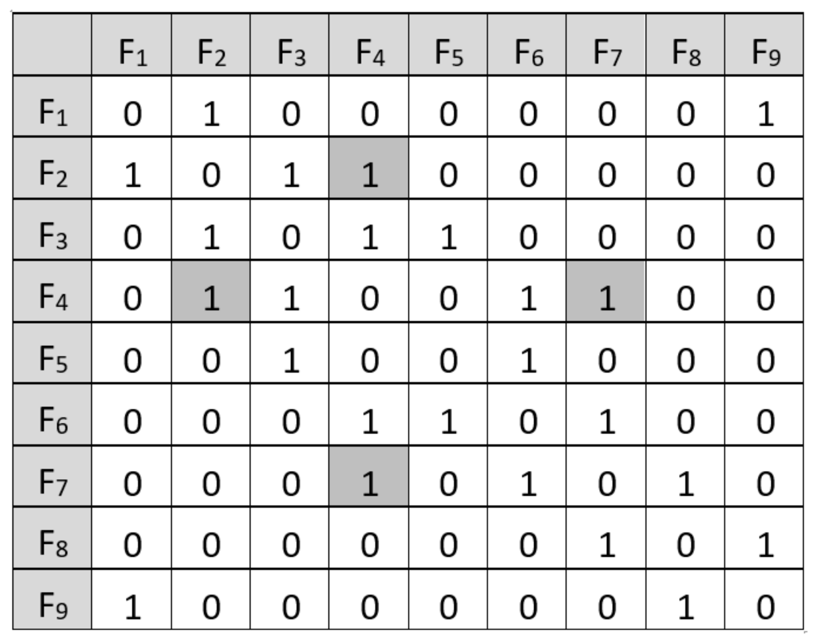
Figure 5 presents the orthogonal projection matrix for the front view shown in Figure 4. As can be seen, vertices F₄–F₆ form an edge, but so do vertices F₄–F₇. The same applies to vertices F₄–F₂ and F₄–F₃. The formula for the number of edges would hold if vertices F₄–F₃ and F₄–F₆ formed edges but F₄–F₇ and F₄–F₆ did not, and then it would be an undirected graph. However, the 3D model is unknown, and whether there is, for example, an edge F₄–F₇ can only be determined by considering hidden edges and a series of vertex relationship tests and calculations, which is difficult to perform for more complex models. Therefore, the assumption is introduced that the orthogonal projection matrix must include projections of all possible surfaces that the 3D model can have in a direction normal to the projection plane, which are defined for the example in Figure 4 by vertices 1-2-4-6-7-8-9, 1-2-3-5-6-7-8-9, and 3-4-6-5.

Following the previous discussion, new rules were introduced into the model. These rules establish a new coordinate, denoted as $c\in x,y,z, \mathrm{that} \mathrm{find} \mathrm{all} \mathrm{points} V_i\in S \mathrm{such} \mathrm{that}: c_i=C,\hspace{1em}\forall i\in I$, which states that if there are three or more points where one specific coordinate remains constant, then any pair of these points can be connected by a valid edge, as follows:

• Let $S=V_1,V_2,\dots ,V_n, \mathrm{where} V_i=\left(x_i,y_i,z_i\right) \mathrm{for} i=1,2,\dots ,n.$
• $\mathrm{For} \mathrm{a} \mathrm{specific} \mathrm{coordinate} c\in x,y,z, \mathrm{find} \mathrm{all} \mathrm{points} V_i\in S \mathrm{such} \mathrm{that}: c_i=C,\hspace{1em}\forall i\in I,$ where C is a constant. $I\subseteq \{1,2,\dots ,n\}$
• $\mathrm{If} \left|I\right|\ge 3$ then all points in the subset: $Sc=Vi:i\in I$ can form valid edges E.

The number of valid edges now can be calculated using the formula for the binomial coefficient

$$E=\left(\begin{array}{c}\left|I\right|\\ 2\end{array}\right)={\displaystyle \frac{\left|I\right|\left(\left|I\right|-1\right)}{2}},\hspace{0.33em}\hspace{0.33em}\hspace{0.33em}\mathrm{if} \left|I\right|\ge 3,$$

where each edge corresponds to a pair of points., i.e., representing several ways to select a pair of points from $\left|I\right|$. Now, a completely defined way of forming a matrix of orthogonal projections is given. In addition to the matrix shown in Figure 5, for each projection, a sequence of vertex coordinates is defined and shown in

Table 1. Vertex coordinate array for front projection.

	X	Z
F1	X1	Z1
F2	X2	Z2
F3	X3	Z3
F4	X4	Z4
F5	X5	Z5
F6	X6	Z6
F7	X7	Z7
F8	X8	Z8
F9	X9	Z9

for the example of the projection from Figure 4. In the same way, projection matrices and vertex coordinate arrays are formed for the other two orthogonal projections.

Now, three square adjacency matrices are defined, representing orthogonal projections $AdjA \mathrm{is} \mathrm{an} n_A\times n_A \mathrm{matrix}, AdjB \mathrm{is} \mathrm{an} n_B\times n_B \mathrm{matrix}, AdjC \mathrm{is} \mathrm{an} n_C\times n_C \mathrm{matrix}.$ Each matrix corresponding to the to the number of vertices in the respective projection.

For each orthogonal projection, a coordinate array is associated: $V_A=V_{A1},V_{A2},\dots ,V_{A_{n_A}},\hspace{0.33em}\hspace{0.33em}\hspace{0.33em}{V}_B=V_{B1},V_{B2},\dots ,V_{B_{n_B}},\hspace{0.33em}\hspace{0.33em}\hspace{0.33em}{V}_C=V_{C1},V_{C2},\dots ,V_{C_{n_C}}$ where the length of each array $\left(\left|V_A\right|=n_A,\hspace{0.33em}\hspace{0.33em}\hspace{0.33em}\left|V_B\right|=n_B,\hspace{0.33em}\hspace{0.33em}\hspace{0.33em}\left|V_C\right|=n_C\right)$ corresponds to the dimension of the associated adjacency matrix. With these definitions, the symmetric adjacency matrix describes the connectivity (edges) of vertices in each projection and coordinate arrays provide the spatial locations of the vertices in their respective views. Now, a 3D model is given with:

$$M=\left\{AdjA,VA,AdjB,VB,AdjC,VC\right\}$$

This formulation sufficiently describes each orthogonal projection to proceed with the identification of candidate vertices and the formation of a pseudo-wireframe model.

Table 2. Comparative overview of topology representations in 3D reconstruction methods.

Representation Method	Input Structure	Geometry Independence	Supports Curved edges	Suitability for GA	Complexity Level
Edge list	List of connected points	✕ Limited	No	Medium	Medium
B-Rep/CSG	Surfaces and operations	No	Partial	No	High
Image-based/Raster methods	Pixel-based shape data	No	No	No	Medium/High
Graph matching	Labeled graphs	Partial	With conditions	Yes	High
Symmetric adjacency matrix (This paper)	Binary vertex–vertex topology	Yes	Partial, to be tested for complex curves	Optimized	Low/Structured

provides a comparative overview of commonly used topology representations in 3D model reconstruction. This highlights the advantages of the proposed method over traditional edge-based, raster, and graph-matching approaches.

As seen in Table 2, the symmetric adjacency matrix offers an optimal balance of generality, simplicity, and GA compatibility, making it a robust foundation for 3D reconstruction from engineering drawings.

The following pseudocode presents the process of converting a DXF file into a symmetric adjacency matrix, encapsulating the previously described methodology in a clear, step-by-step format (Algorithm 2).

Algorithm 2 Generation of a symmetric adjacency matrix from DXF orthographic pro-jections.

Pipeline for converting DXF data into a symmetric adjacency matrix Input: DXF file containing 2D orthographic projections (front, top, left) Output: Symmetric adjacency matrices for each projection Import and parse the DXF file (ASCII format) Segment the drawing into three orthographic views based on spatial grouping For each view:  1. Identify geometric entities: LINE, ARC, CIRCLE  2. Extract start and end points for each entity  3. Create vertex list by grouping nearby points (with tolerance ε)  4. Generate edge list by mapping entities to vertex pairs  5. Build adjacency matrix: set Adj[i][j] = 1 if an edge connects vertex i and j Ensure symmetry: enforce Adj[i][j] = Adj[j][i] Validate: check consistency rules (number of edges, symmetry, no self-loops)

3.4. Generation of Candidate Vertices and a Pseudo Wireframe Model

The formation of a pseudo-wireframe model was initially described and formalized in [3,4], with an additional method presented in [5]. In this paper, a new method for forming a pseudo wireframe model will be presented. The initial step involves defining all potential vertices for the pseudo-wireframe model, which entails several sub steps. The goal is to identify all potential 3D vertices $V_i^{3D}=\left(x_i,y_i,z_i\right)$ that are consistent across all three orthogonal projections. This is achieved by verifying compatibility between the projection based on the given coordinates. Based on the discussions in Section 3.3, a step-by-step procedure for generating candidate vertices is provided:

• Iterate over all combinations: For each combination of indices (i, j, k),$i\in 1, 2, \dots ,{ n}_A,\hspace{0.33em}\hspace{0.33em}\hspace{0.33em}j\in 1, 2, \dots ,{ n}_B,\hspace{0.33em}\hspace{0.33em}\hspace{0.33em}k\in 1, 2,\dots , n_C$ evaluates the following condition:
• Compatibility check: A vertex (x, y, z)) is a candidate if the following conditions are met:

  $$\begin{gathered} \left|x_{Ai}-x_{Bj}\right|=0 \\ \left|y_{Bj}-x_{Ck}\right|=0 \\ \left|y_{Ai}-y_{Ck}\right|=0 \end{gathered}$$
• Generate candidate vertex: If the conditions hold, compute the candidate vertex as $x=x_{Ai}$, $y=y_{Bj}$, $z=y_{Ck}$.
• Store candidate: Add the candidate vertex $V^{3D}=\left(x,y,z\right)$ to the result set: $V_{\mathrm{candidates}}^{3D}$
• Output: The final result is the set of all valid candidate vertices: $V_{\mathrm{candidates}}^{3D}=V_1^{3D},V_2^{3D},\dots ,V_m^{3D},$ where $m\le n_A\cdot n_B\cdot n_C$ depends on the number of valid combinations.

Following the logic that an orthogonal projection is represented by a symmetric adjacency matrix and a set of vertex coordinates, the same applies to the pseudo-wireframe 3D model. Therefore, it is necessary to define the matrix Adj as the symmetric adjacency matrix of edges in the 3D model. The procedure is relatively simple and evaluates whether an edge exists between two vertices in a 3D model based on their adjacency in the spatial symmetric adjacency matrix and their projections in the three orthogonal views. An edge is considered to exist within a 3D model if and only if its representation is present in all orthogonal projections. The visual representation of an edge in these projections can vary, appearing as either a line or a point. This variability is determined by the edge’s spatial orientation relative to the coordinate planes—specifically, whether it is orthogonal or parallel to them. Generally, if an edge is neither orthogonal nor parallel to any coordinate plane, it will manifest as a line in all three projections.

For each pair of candidate vertices $\left(v_i,v_j\right)$, their corresponding Adj[i][j] is determined as follows:

• Map Vertices to Projections: Project vertices $v_i$ and $v_j$ onto the orthogonal planes:

  $$\begin{gathered} P_1=\left(x_i,z_i\right)\wedge P_2=\left(x_j,z_j\right) \mathrm{for} \mathit{xz} \mathrm{plane} \\ {P}_3=\left(x_i,y_i\right)\wedge P_4=\left(x_j,y_j\right) \mathrm{for} \mathit{xy} \mathrm{plane} \\ {P}_5=\left(y_i,z_i\right)\wedge P_6=\left(y_j,z_j\right) \mathrm{for} \mathit{yz} \mathrm{plane} \end{gathered}$$

  Using these projections, locate the corresponding indices in the projection vertex arrays:

  $$\begin{gathered} I_1=IndexOf\left(P_1,VA\right), I_2=IndexOf\left(P_2,VA\right) \\ { I}_3=IndexOf\left(P_3,VB\right), I_4=IndexOf\left(P_4,VB\right) \\ {I}_5=IndexOf\left(P_5,VB\right),{ I}_6=IndexOf\left(P_6,VB\right) \end{gathered}$$
• Edge existence check in projections: Evaluate whether edges exist between the projected vertices in their respective adjacency matrices:

  $$\begin{gathered} E_A=\left(\mathit{AdjA}\left[I_1\right]\left[I_2\right]>0\right)\vee \left(\left(I_1=I_2\right)\wedge \left(\mathit{AdjA}\left[I_1\right]\left[I_2\right]=0\right)\right) \\ {E}_B=\left(\mathit{AdjB}\left[I_3\right]\left[I_4\right]>0\right)\vee \left(\left(I_3=I_4\right)\wedge \left(\mathit{AdjB}\left[I_3\right]\left[I_4\right]=0\right)\right) \\ {E}_C=\left(\mathit{AdjC}\left[I_5\right]\left[I_6\right]>0\right)\vee \left(\left(I_5=I_6\right)\wedge \left(\mathit{AdjC}\left[I_5\right]\left[I_6\right]=0\right)\right) \end{gathered}$$
• Spatial edge update: Update the spatial symmetric adjacency matrix Adj for the edge [i][j]

  $$\begin{gathered} E_A\wedge E_B\wedge E_C\Rightarrow Adj\left[i\right]\left[j\right]=1 \\ \neg \left(E_A\wedge E_B\wedge E_C\right)\Rightarrow Adj\left[i\right]\left[j\right]=0 \end{gathered}$$

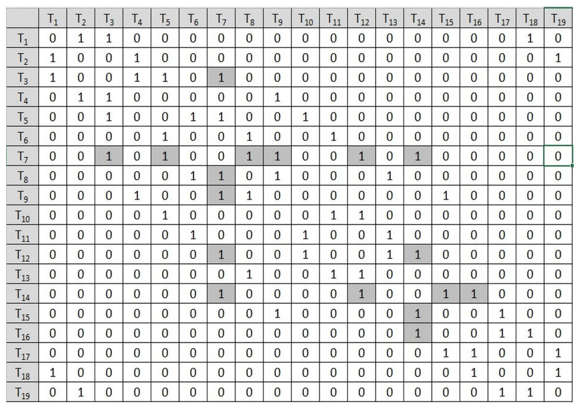
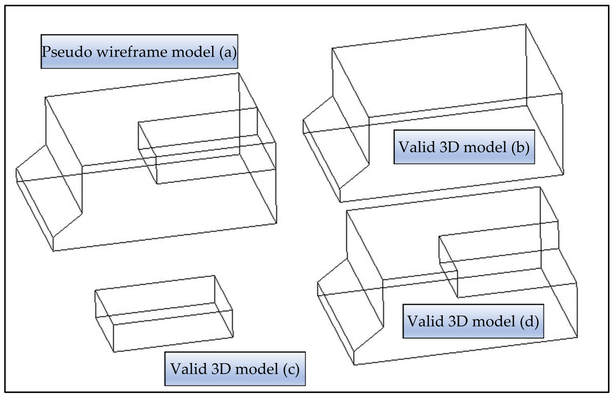
The 3D model is now represented by $M=\left\{Adj,V_{ \mathrm{candidates}}^{3D}\right\}$, which defines all possible solutions of the pseudo-wireframe model. Figure 6 and Figure 7 illustrate the reconstruction process for the part shown in Figure 1. Figure 6 presents the symmetric adjacency matrix AdjA, while Figure 7 shows all possible 3D models generated from this matrix and the corresponding candidate vertices. Figure 7a shows a pseudo-wireframe 3D model that encompasses three valid reconstruction candidates, as their geometries are consistent with the input projections. Among them, the model in Figure 7d is the one intended for reconstruction, while the models shown in Figure 7b,c are also geometrically valid solutions; however, they do not represent the target 3D reconstruction and must therefore be discarded during the process.

Human designers often approach engineering drawings by attempting to mentally reconstruct the 3D object through identification of geometric relationships across multiple views. This process typically involves a sequence of intuitive evaluations and repeated adjustments, which continues until a coherent 3D representation is formed in their minds [6].

The process of 3D wireframe model reconstruction can be defined as a process of adding or removing candidate vertices and their corresponding edges while respecting constraints related to geometric consistency until a solution is obtained that satisfies predefined criteria. This defined process of 3D wireframe model reconstruction represents a standard optimization problem, for the realization of which it is necessary to define a mathematical model that should be independent of the optimization method.

3.5. Mathematical Formulation of the Proposed Model

• Input variables

• Orthogonal projection symmetric adjacency matrices and their dimensions:

• $AdjA\in {\left\{\mathrm{0,1}\right\}}^{n_{A}x{n}_A}$ adjacency matrix for the front projection;
• $AdjB\in {\left\{\mathrm{0,1}\right\}}^{n_{B}x{n}_B}$ adjacency matrix for the top projection;
• $Adj\mathrm{C}\in {\left\{\mathrm{0,1}\right\}}^{n_{\mathrm{C}}x{n}_{\mathrm{C}}}$ adjacency matrix for the left projection.

2.

Vertex coordinates of projections:

• $V_A={\left\{\left(x_i^A,z_i^A\right)\right\}}_{i=1}^{n_A}$ coordinates of vertices in front projection;
• $V_{\mathrm{B}}={\left\{\left(x_i^{\mathrm{B}},{\mathrm{y}}_i^{\mathrm{B}}\right)\right\}}_{i=1}^{n_{\mathrm{B}}}$ coordinates of vertices in top projection;
• $V_C={\left\{\left(y_i^C,z_i^C\right)\right\}}_{i=1}^{n_C}$ coordinates of vertices in left projection.

1.

Coordinate vertex set and connectivity:

• ${\mathrm{V}}_{\mathrm{K}}={\left\{\left(x_i^K,y_i^K,z_i^K\right)\right\}}_{i=1}^{N_K}$ 3D candidate vertex coordinates;
• $Adj\in {\left\{\mathrm{0,1}\right\}}^{N_{K}x{N}_K}$ symmetric adjacency matrix for pseudo wireframe model.

2.

Bounds on the number of vertices:

• $n$ ≤ N ≤ NK, n = max$(n_A,n_B,n_C)$.

3.

Target number of edges:

• Marked as T where T is derived from Adj.

• Control variables of the mathematical model

In addition to the observed model’s input variables, it is necessary to define a vector of control variables, that is, variables that describe the optimization objectives stated.

$$x_i\in \left\{0, 1\right\}, i=\mathrm{1,2}, ..., N_K$$

(1)

where $x_i$—vertex inclusion indicator is a binary variable indicating whether vertex i is included in the 3D model

$$e_{ij}\in \left\{0, 1\right\}, i,j=\mathrm{1,2}, ..., N_K$$

(2)

where $e_{ij}$—edge inclusion indicator is a binary variable indicating whether edge (i, j) is included in the 3D model

$${Adj}^{curr}(x_i,e_{ij})\in \left\{0, 1\right\}, i,j=\mathrm{1,2}, ..., N_K$$

(3)

where ${Adj}^{curr}$—reduced symmetric adjacency matrix is a binary variable representing the current 3D model using $x_i$ and $e_{ij}$.

• The objective function

The objective function of the mathematical model represents the criteria of optimization. As mentioned earlier the goal is to measure the difference between current 3D model and the target 3D model where target 3D model is represented with orthogonal projections. However, determining this difference is not sufficient, and even has a smaller impact on the optimization result, because orthogonal projections encompass all possible model solutions that are geometrically consistent. Therefore, in addition to measuring the difference between projections, it is necessary to introduce an additional parameter into the objective function. Figure 7 clearly shows that the solutions differ in the number of edges, although all edges are displayed in a pseudo-wireframe model. The target number of edges cannot be the number of edges of the pseudo-wireframe model because valid models have fewer edges. It is necessary to determine the difference between the number of edges of ${Adj}^{curr}(x_i,e_{ij})$ and the target number of edges that the model to be recognized has. This can be achieved with the following procedure:

• Identify the vertex with the highest weight (most edges) in Adj;
• Set all entries in the corresponding row and column of that vertex 0 in Adj;
• Adj = ${Adj}^{curr}(x_i,e_{ij})$;
• Repeat steps 1–3 until each row and column in Adj has either 0 or 3 non-zero entries but without violating geometric consistency;
• The sum off all 1-values in Adj after processing is the target number of edges T.

When there is more than one goal to achieve during the optimization process, there are several ways to define an objective function [21] without entering in space of multi-objective optimization. Finally, objective function $F\left(x,e\right)$ can be written as:

$$\mathit{min}\left(F\left(x,e\right)\right)=\mathit{min}({\omega }_1·F_N\left(x,e\right)+{\omega }_2·\left(F_T\left(x,e\right)\times p\right))$$

(4)

$$F_N\left(x, e\right)={‖AdjA-ProjA\left(x, e\right)‖}_F^2+{‖AdjB-ProjB\left(x, e\right)‖}_F^2+{‖AdjC-ProjC\left(x, e\right)‖}_F^2$$

(5)

$$F_T\left(x,e\right)={\left(E\left(x,e\right)-T\right)}^2$$

(6)

where $F_N\left(x, e\right)$ is the Frobenius norm between goal projections adjacency matrices and projection adjacency matrices of orthogonal projections of current 3D model ProjA, ProjB, ProjC. $F_T\left(x,e\right)$ is the difference between the total number of edges of a current 3D model and the target number of edges, ${\omega }_1$, and ${\omega }_2$ are weighting coefficients that determine weights for the two objectives in the overall objective function. Vector $\overrightarrow{p}$ is a penalty vector and will be explained later.

• Constraints of a mathematical model

The vertex–edge consistency constraint ensures that an edge $e_{ij}$ can only exist if both of its corresponding vertices i and j are included in the model. This is critical for maintaining logical consistency in the graph structure of the 3D model.

$$e_{ij}\le x_i,e_{ij}\le x_j,\forall i,j.$$

(7)

This constraint ensures that edges cannot “float” without being connected to valid vertices. In other words, if a vertex is excluded from the model, all edges connected to that vertex must also be excluded. This maintains the integrity of the graph structure during the iterative procedure.

The geometric consistency constraint prevents the removal of vertices and their associated edges if the result violates the required geometric structure during the iterative procedure. Specifically, it is required that the symmetric adjacency matrix ${Adj}^{curr}(x_i,e_{ij})$ after removing a vertex (and its corresponding edges) must have a non-zero-sum, ensuring that at least some connections remain.

$${\displaystyle \sum _{i,j}{e}_{ij}}\cdot x_i\cdot x_j\ne 0$$

(8)

The minimum and maximum vertices constraint ensures that the reconstructed 3D model contains only vertices within the permissible range defined by the input data. This constraint is expressed as:

$$n\le {\displaystyle \sum _{i=1}^K{x}_i}\le N_K$$

(9)

The edge connectivity constraint ensures that if an edge $(e_{ij}=1)$ exists, then both vertices $x_i$ and $x_j$ are present. This adds a lower bound on the sum $x_i$ + $x_j$, reinforcing that both vertices must exist for the edge to be valid.

$$x_i+x_j\ge 2\cdot e_{ij}, \forall i,j.$$

(10)

3.6. Introduction to the Proposed GA for 3D Wireframe Model Reconstruction

An acceptable 3D wireframe model can be defined as a selected subset of vertices derived from a larger set, structured to represent a 3D object while adhering to the constraints specified in a corresponding integer programming formulation. Genetic algorithms (GAs), as modern metaheuristic optimization techniques, are particularly well suited for addressing such problems due to their strong capability to converge toward a global optimum with high probability in most cases [22].

It is important to emphasize that the performance of a GA is significantly influenced by the choice of crossover and mutation operators [23]. However, for the model under consideration, the most critical component is the penalization of candidate solutions based on their validity. Only feasible solutions, as defined by the problem’s constraints, are accepted in the model, and further explanation will be provided in subsequent sections.

Numerous variants of genetic operators exist in the literature, many of which can be tailored to accommodate specific characteristics of the problem at hand, thereby enhancing the adaptability of the GA. Since the general functioning of GAs is well established and extensively documented, this work provides only brief definitions of the fundamental GA components, contextualized within the proposed model.

In this model, a gene corresponds to a vertex (denoted as xix_ixi) and serves as the basic unit of encoded information. An individual or chromosome is a combination of such genes, representing a candidate 3D wireframe model. A population refers to the collection of all such individuals, i.e., the full set of acceptable 3D wireframe configurations.

Parents are two feasible 3D wireframe models that participate in reproduction to generate new candidate models. The fitness function evaluates the quality of each model; in this context, it is based on the discrepancy between the orthogonal projections derived from the engineering drawing and those generated from the candidate model, along with the difference in the number of edges. This is formally defined in Equation (4) of the mathematical model.

The crossover operator is responsible for combining two parent solutions (analogous to tool paths) to produce a new offspring. The mutation operator, on the other hand, modifies one or more genes within a single individual with the aim of introducing variability and potentially discovering superior solutions. The specific implementation of these genetic operators, as applied in the proposed model, will be detailed in later sections.

3.7. Chromosome Representation and Decoding: Initial Population

The initial phase of any genetic algorithm involves selecting a suitable encoding scheme to represent candidate solutions. Choosing the right representation is paramount, as it impacts every subsequent stage of the GA’s execution. In our framework, this entails encoding each chromosome as a binary vector, with the specifics dictated by the underlying model. The approach is based on a binary chromosome representation where each gene corresponds to a vertex in the model, and the total number of genes equals the dimension of the symmetric adjacency matrix. A gene’s value indicates the inclusion (1) or exclusion (0) of a vertex in the reconstructed model. Each vertex is assigned a weight based on the number of edges connected to it. Typically, vertices in most mechanical parts have a maximum of three edges, but the pseudo-wireframe model may include vertices with higher connectivity (e.g., four, five, or more edges).

The reconstruction process differentiates between acceptable and valid individuals. Acceptable individuals are those maintaining geometric consistency, making them suitable for the initial population. Valid individuals are obtained through the evolutionary process, where crossover and mutation operators improve the population by refining geometric and structural consistency. Geometric consistency is maintained by ensuring that the sum of all elements in the symmetric adjacency matrix is not zero after the removal of any vertex or its edges.

The chromosome is decoded into the current symmetric adjacency matrix, reflecting the connectivity of the vertices included in the current individual. This matrix is compared with the original adjacency matrix to measure projection consistency and edge count.

The initial population includes chromosomes that do not violate geometric consistency. During the evolutionary process, vertices with higher weights are more likely to be excluded, provided their removal does not disrupt the model’s structural integrity. The optimization ensures convergence to a valid model. For a model with 19 vertices (as shown in Figure 7), the chromosome is represented as a binary vector (11).

x = [1, 0, 1, 1, 0, 1, 1, 1, 0, 0, 1, 1, 1, 1, 0, 0, 1, 1, 0]

(11)

w = [3, 3, 4, 3, 4, 4, 3, 6, 4, 4, 3, 3, 4, 3, 4, 3, 3, 3, 3]

(12)

The weights are calculated based on the adjacency matrix Adj (Figure 6), resulting in the weight vector $\overrightarrow{\varpi }$ (12). Each gene is not only defined by its binary value but also by its position within the chromosome and its associated entry in the adjacency matrix. Beyond its value, a gene is further specified by an index denoting its position within the chromosome and its corresponding entry in the connectivity matrix. Gene selection, for creating a chromosome, specifically the inclusion of vertex ij in the model, is entirely stochastic taking into account only the constraint given in (9), rendering the example provided in (11) incompatible with any valid solution in the beginning of the evolution process. The initial population is formed as an array of chromosomes, without the implementation of other constraints except (9).

3.8. Fitness Calculation: Penalization of Acceptable Chromosomes

The fitness function plays a central role in steering the GA toward geometrically valid and topologically optimal 3D reconstructions. It integrates a projection consistency component—quantified using the Frobenius norm—with a penalty term that accounts for deviations from the expected number of edges. Each chromosome is assessed according to these dual criteria, and only individuals that satisfy predefined geometric constraints are retained as valid solutions. This fitness evaluation framework promotes convergence toward a unique, structurally coherent configuration, thereby ensuring topological consistency across projections within a finite number of evolutionary iterations.

The fitness function evaluates the quality of a chromosome in the GA, guiding the evolutionary process toward reconstructing the 3D wireframe model. It is defined with Equation (4), where:

• $F_N\left(x,e\right)$: Frobenius norm-based projection consistency measure, evaluating how well the reconstructed model matches the initial orthogonal projections.
• $F_T\left(x,e\right):$ Edge count consistency measure, assessing the difference between the current number of edges and the target edge count.
• ${\omega }_1 \mathrm{a}\mathrm{n}\mathrm{d} {\omega }_2$: Weighting coefficients balancing the importance of $F_N \mathrm{a}\mathrm{n}\mathrm{d} F_T.$ In the context of the observed model ${\omega }_1=0.3 \mathrm{a}\mathrm{n}\mathrm{d} {\omega }_2=0.7$.
• $\overrightarrow{p}$: Penalty vector, calculated as the product of the binary chromosome $x$ and the weight vector $\overrightarrow{\varpi }$, which represents the number of edges connected to each vertex.

The penalty mechanism is implemented through the penalty vector $\overrightarrow{p}$ discourages chromosomes with vertices that have excessive edge weights (w > 3). Each gene $x_{\mathrm{i}}$ is penalized with a factor proportional $10\cdot w_i \mathrm{if} w_i>3$. This ensures that vertices with high connectivity do not dominate the solution, as they often represent unrealistic or invalid structures in the context of the model. A lower fitness value indicates a better individual. Poorly penalized chromosomes are less likely to be selected as parents, preventing them from evolving further. This introduces a sort of genetic engineering into the algorithm by focusing the evolutionary process on improving acceptable solutions into valid ones.

• Example of fitness evaluation:

x = [1, 0, 1, 1, 0, 1, 1, 1, 0, 0, 1, 1, 1, 1, 0, 0, 1, 1, 0]

w = [3, 3, 4, 3, 4, 4, 3, 6, 4, 4, 3, 3, 4, 3, 4, 3, 3, 3, 3]

The penalty vector $\overrightarrow{p}$ is computed by multiplying $x \mathrm{a}\mathrm{n}\mathrm{d} \varpi$ followed by penalizing genes with $w_i>3$

p = [3, 0, 40, 3, 0, 40, 3, 60, 0, 0, 3, 3, 40, 3, 0, 0, 3, 3, 0]

• $F_N\left(x,e\right)$ = 0.2 (normalized projection consistency for example);
• $F_T\left(x,e\right)$ = 0.1 (normalized edge count difference for example);
• ${\omega }_1=0.5 \mathrm{a}\mathrm{n}\mathrm{d} {\omega }_2=0.5$.

$$F(x,e)=0.5\cdot 0.2+0.5\cdot 20.2=10.2$$

Computing and summing elements of p gives up $p\cdot F_T(x,e)=20.2$

Final fitness: $F(x,e)=0.5\cdot 0.2+0.5\cdot 20.2=10.2$

Chromosomes with penalized vertices $(\mathrm{e}.\mathrm{g}., w_3, w_5, w_6, w_8)$ contribute to higher fitness values. The algorithm favors chromosomes with lower weights, as they are closer to valid configurations.

3.9. Selection of Parents, Crossover, and Mutation Operator

In our GA framework, a pair of feasible 3D wireframe models (“parents”) is chosen to generate a new candidate solution. Parent selection is achieved by ranking models according to their fitness values; those with the lowest fitness scores are marked as parents and advanced to the crossover pool. This selection cycle repeats until the predefined number of parent pairs—determined by the algorithm’s population size—has been reached.

Crossover then combines genetic information from two parent chromosomes to produce offspring. Each child inherits a mixture of binary-encoded genes from both parents, and specialized crossover operators (e.g., one-point, two-point, uniform) appropriate for binary strings are applied to effect this exchange. A concise review of the most widely used crossover techniques can be found in [23,24,25]. For the observed model, single-point crossover is chosen. The operation of single-point crossover is illustrated by the following example:

• Parent 1: $x^1$= [1, 0, 1, 1, 0, 1, 1, 0, 0, 1];
• Parent 2: $x^2$= [0, 1, 0, 0, 1, 0, 1, 1, 1, 0].

A random crossover point is selected. For this example, let the crossover point be after the 5th gene (index 5). The chromosomes are split into two segments:

• Parent 1: [1, 0, 1, 1, 0]∣[1, 1, 0, 0, 1];
• Parent 2: [0, 1, 0, 0, 1]∣[0, 1, 1, 1, 0].

The offspring are generated by swapping the segments:

• Offspring 1: [1, 0, 1, 1, 0] + [0, 1, 1, 1, 0] = [1, 0, 1, 1, 0, 0, 1, 1, 1, 0];
• Offspring 2: [0, 1, 0, 0, 1] + [1, 1, 0, 0, 1] = [0, 1, 0, 0, 1, 1, 1, 0, 0, 1].

Each gene in the chromosome corresponds to a vertex in the model. The value 11 means the vertex is included, and 0 means it is excluded. The crossover combines the structural characteristics of both parents. For instance:

• Offspring 1 inherits the first half of Parent 1 and the second half of Parent 2.
• Offspring 2 inherits the first half of Parent 2 and the second half of Parent 1.

After generating offspring, their fitness is evaluated using the fitness function, where penalties $\overrightarrow{p}$ are applied if vertices with high edge weights are included. Single-point crossover creates new combinations of genes, promoting diversity in the population. In the 3D model reconstruction problem, Parent 1 and Parent 2 might represent partial solutions that preserve different structural features of the model. By combining their chromosomes, offspring may inherit valid structural properties from both, leading to improved fitness and closer approximations to the target model.

The mutation operator chosen is an inversion operator. It is a mutation mechanism used in GA to introduce variability into the population. It works by flipping the value of a randomly selected gene in a chromosome.

• If the gene’s value is 1, it is changed to 0, and vice versa.
• The operation is triggered based on a predefined mutation rate, ensuring controlled and rare alterations to preserve promising solutions while exploring new ones.

This operator prevents premature convergence by injecting diversity into the population and helps the algorithm explore new areas of the solution space. In the context of 3D model reconstruction, inversion can add or remove vertices from the model, refining the population towards geometrically consistent and valid solutions.

A known limitation of GA is its tendency to converge toward a local optimum, which may not necessarily yield a valid 3D model reconstruction. This is compounded by the fact that the GA’s execution is typically constrained by a predefined number of generations. Furthermore, given that the symmetric adjacency matrix encoding the 3D model’s edges encompasses all potentially valid solutions, it becomes imperative to establish supplementary termination criteria for the recognition process. Specifically, the reconstructed 3D model must exhibit geometric consistency, ensuring the absence of edge overlaps and the uniqueness of the solution. Consequently, an iterative GA execution is required until a single, geometrically sound solution is achieved, devoid of any edge ambiguities.

3.10. Pseudo Code of Proposed GA

The genetic algorithm implementation requires four primary configuration parameters: (1) population cardinality, (2) quantity of parent individuals selected for reproduction, (3) probability of genetic mutation, and (4) maximum evolutionary cycles. The computational process begins by instantiating the initial population and evaluating each candidate solution’s fitness. Through iterative generational advancement, the algorithm performs selective breeding using single-point crossover operations, introduces random mutations, and continuously monitors for topological validity until convergence criteria are satisfied (Algorithm 3).

Algorithm 3 Evolutionary reconstruction framework.

PseudoCode Evolutionary Reconstruction Framework Parameters:  - POP_SIZE: Integer (Population cardinality)  - NUM_PARENTS: Integer (Reproductive pool size)  - MUT_RATE: Float ∈ [0, 1] (Variation probability)  - MAX_GEN: Integer (Termination condition) 1. INITIALIZATION:   population = GENERATE_RANDOM_POPULATION(POP_SIZE)   EVALUATE_FITNESS(population)   current_gen = 1 2. GENERATIONAL LOOP:   WHILE current_gen ≤ MAX_GEN:    selected_parents = BestFitness(population, NUM_PARENTS)    offspring = EMPTY_SET()       WHILE SIZE(offspring) < (POP_SIZE-NUM_PARENTS):      parent1, parent2 = SELECT_PAIR(selected_parents)      child = SINGLE_POINT_RECOMBINATION(parent1, parent2)      IF RANDOM() < MUT_RATE:       child = APPLY_MUTATION(child)          ADD_TO_SET(offspring, child)       population = COMBINE(selected_parents, offspring)    EVALUATE_FITNESS(population)    current_gen += 1       IF VALID_SOLUTION_EXISTS(population) AND      NOT HAS_EDGE_CONFLICTS(population):      BREAK 3. TERMINATION:   RETURN BEST_SOLUTION(population)

4. Experimental Results

The mathematical model provided in Section 2 is realized through application in which the previously presented GA is implemented and is written in the object-oriented programming language Delphi. It is independent executable software platform and in the following paragraph, a brief overview of the main screen and the functionality of the application is provided.

4.1. Brief Overview of the Software Platform

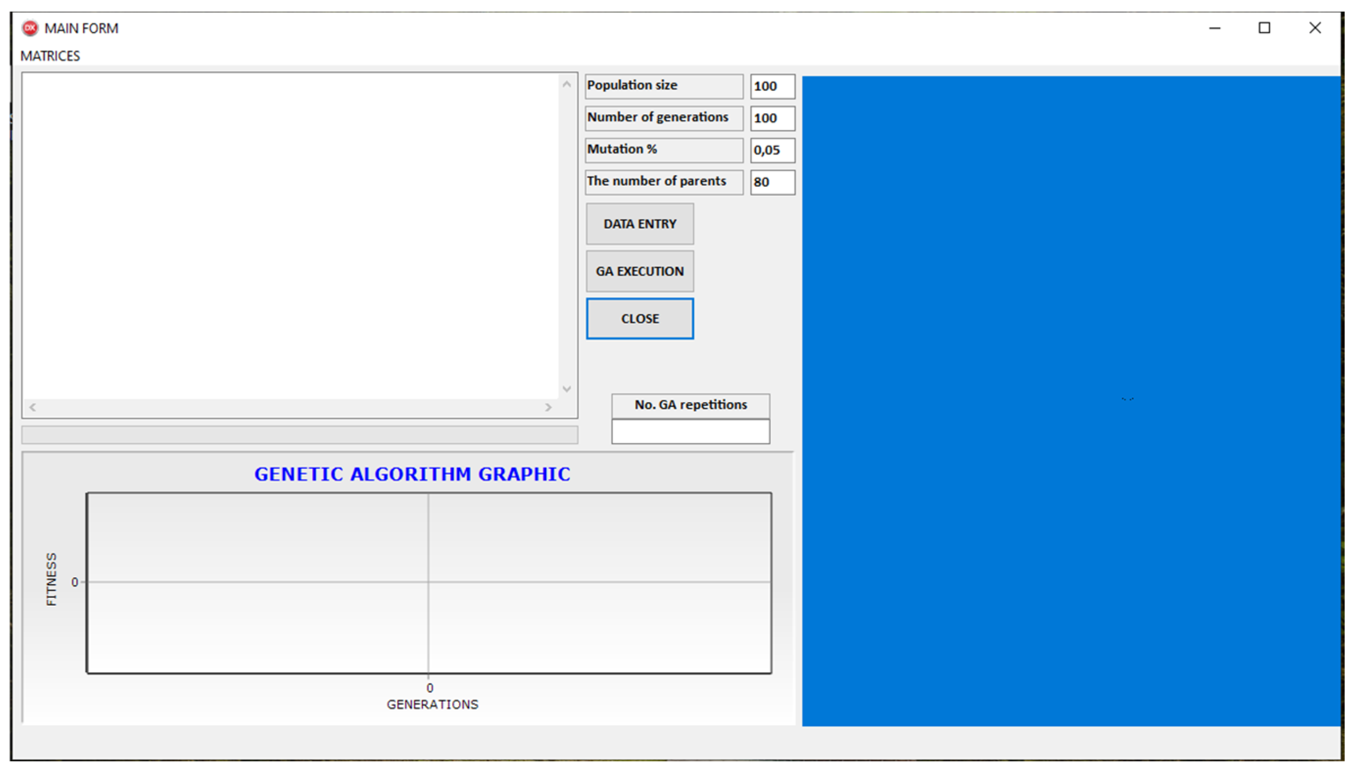
Figure 8 presents the application’s initial screen. In the middle of the main form there are command buttons for the following:

• Data entry (loading orthogonal symmetric projection matrices and vertex arrays);
• Executing the GA;
• Closing the application.

The left side of the input form displays the GA execution results, while the bottom half visualizes the GA process. The left half of the main form displays the results of the GA execution, the initial symmetric adjacency matrix of the pseudo-wireframe model, the fitness of each best individual in the generation, and the symmetric adjacency matrix of the best solution obtained at the end of the GA execution. In the middle of the main form, there is information about the number of GA executions up to the moment of obtaining the best solution, as well as the GA parameters that can be changed. In the right part of the main form, there is a window with a 3D graphical representation of the GA execution, while at the bottom, there is a diagram of the GA execution The application begins by loading orthogonal projections, i.e., DXF files for each view, and forming symmetric adjacency matrices for each projection.

4.2. The Structure and Loading Process of Input Data

The input data consist of pre-generated matrices of orthogonal projections and arrays of vertex coordinates for each projection. The data are stored in *.txt files for each projection, as shown in

Table 3. Sample input structure of projection data stored in plain text files.

Section	Example Content
Projection name	Front
Adjacency matrix size	9 × 9
Adjacency matrix (AdjA)	0 1 0 0 0 0 0 0 1 1 0 1 1 0 0 0 0 0 0 1 1 1 0 0 0 0 0 0 1 1 0 1 1 0 0 0 0 0 0 1 0 1 0 0 0 0 0 0 1 1 0 1 0 0 0 0 0 0 0 1 0 1 0 0 0 0 0 0 0 1 0 1 1 0 0 0 0 0 0 1 0
Vertex coordinates (VA)	0 0 150 0 150 40 150 60 70 40 70 60 20 60 20 25 0 10

.

The first line contains the name of the projection (e.g., Front), followed by the dimension of the matrix AdjA in the format n_A × n_A, and then the adjacency matrix of the front orthogonal projection. Next comes the array of vertex coordinates, and at the end, there is an empty line. This pattern is repeated for the subsequent projections, i.e., AdjB, VB, AdjC and VA, VB and VC.

4.3. Testing Parameters

The proposed solution has been tested on several real models, four of which will be presented here.

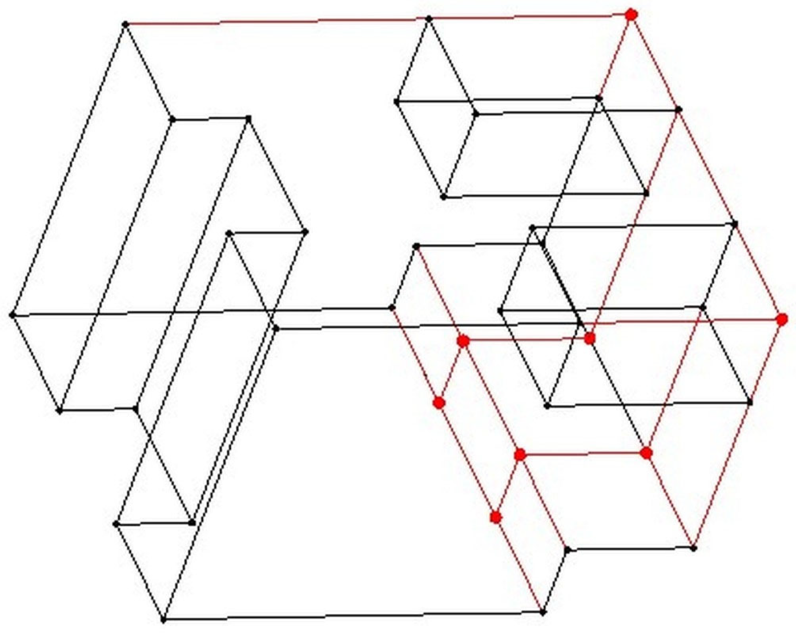
The first, which is simpler, is shown as an example throughout this paper. The second, more complex part, with 40 vertices and 168 edges in the pseudo-wireframe model, is shown in Figure 9 as a solid model and in Figure 10 as a wireframe model. The edges marked in red represent those that do not belong to the real model but to the set of all valid solutions. Also, vertices marked in red are vertices that belong to the candidate set but that do not belong to the vertices of a real 3D model. In

Table 4. The geometric characteristics of tested models.

Model Name	No. Edges 3D Wireframe	No. Vertices 3D Wireframe	No. Edges 3D Real Model	No. Vertices 3D Real Model
PR0003	66	19	27	18
PR0004	168	40	60	32

, the geometric characteristics of both models are provided.

Given that GA results can vary based on input parameters, five GA runs were conducted with different parameter sets.

Table 5. The parameters for the execution of GA.

Name of Parameter	I	II	II	IV	V
Population size	100	200	300	400	500
Number of parents	80	80	240	320	420
Mutation in %	1	1	1	1	1
Number of generations	100	100	100	100	100

presents the parameter values for each run, while

Table 6. Test output parameter list with obtained values for PR0003.

Name of Parameter	I	II	II	IV	V
Fitness	1.1	1.1	1.1	1.1	/
Execution time/computational complexity in sec	2	2	3	4	/
Valid solution obtained (Yes/No)	Yes	Yes	Yes	Yes	/
Solution with double edges	No	No	No	No	/
No. of double edges	/	/	/	/	/
No. of GA repetitions	1	1	1	1	/

and

Table 7. Test output parameter list with obtained values for PR0004.

Name of Parameter	I	II	II	IV	V
Fitness	10.3	10.3	10.3	10.3	10.3
Execution time/computational complexity in sec	60	54	90	94	100
Valid solution obtained (Yes/No)	Yes	Yes	Yes	Yes	Yes
Solution with double edges	No	No	No	No	No
No. of double edges	/	/	/	/	/
No. of GA repetitions	6	4	4	3	3

lists the names of the output parameters with experimental results for PR0003 and PR0004, respectively.

To evaluate the impact of different parameter settings, the GA was run with four (PR0003) and five (PR0004) parameter configurations. The results are tabulated in Table 6 and Table 7, and visualized in Figure 11, Figure 12, Figure 13, Figure 14, Figure 15, Figure 16, Figure 17, Figure 18, Figure 19 and Figure 20. The primary objective was to assess the GA’s ability to converge to valid solutions for complex shapes like PR0004, while restricting the analysis to polyhedral shapes.

The second objective of the experimental testing of the proposed GA was to examine its convergence capability toward valid solutions for geometric solids with cylindrical surfaces. This presents a greater challenge, particularly for GAs [19]. Figure 21 illustrates an example of a 3D solid model of PR0007 with cylindrical surfaces, while Figure 22 shows the experimental results for I parameter group. The testing was conducted using the first four configurations of GA parameters, and the results are presented in

Table 8. Test output parameter list with obtained values for PR0007.

Name of Parameter	I	II	II	IV	V
Fitness	2.4	2.4	2.4	2.4	/
Execution time/computational complexity in sec	2	2	3	4	/
Valid solution obtained (Yes/No)	Yes	Yes	Yes	Yes	/
Solution with double edges	No	No	No	No	/
No. of double edges	/	/	/	/	/
No. of GA repetitions	1	1	1	1	/

. Figure 23 illustrates a more complex, typical industrial part with cylindrical surfaces part tested with the first three configurations of GA parameters, while Figure 24 shows the experimental results for I parameter group. The testing results are presented in

Table 9. Test output parameter list with obtained values for PR0005.

Name of Parameter	I	II	II	IV	V
Fitness	112.20	112.20	112.20	/	/
Execution time/computational complexity in sec	60	86	94	/	/
Valid solution obtained (Yes/No)	Yes	Yes	Yes	/	/
Solution with double edges	No	No	No	/	/
No. of double edges	/	/	/	/	/
No. of GA repetitions	6	4	5	/	/

.

To examine the behavior of the proposed genetic algorithm (GA) under different evolutionary parameter settings, a series of experimental runs was performed on two test cases of increasing complexity—PR0003 and PR0004. Figure 11, Figure 12, Figure 13, Figure 14, Figure 15, Figure 16, Figure 17, Figure 18, Figure 19 and Figure 20 provide a detailed visualization of the algorithm’s execution across five parameter groups for each model, with particular focus on convergence characteristics, solution accuracy, and structural validity of the reconstructed wireframe models.

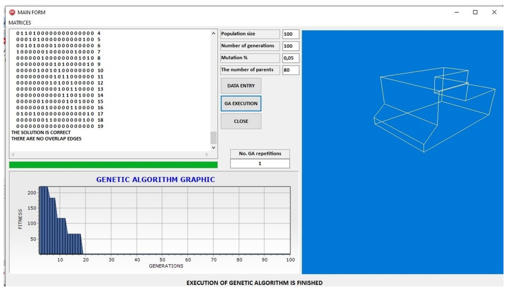
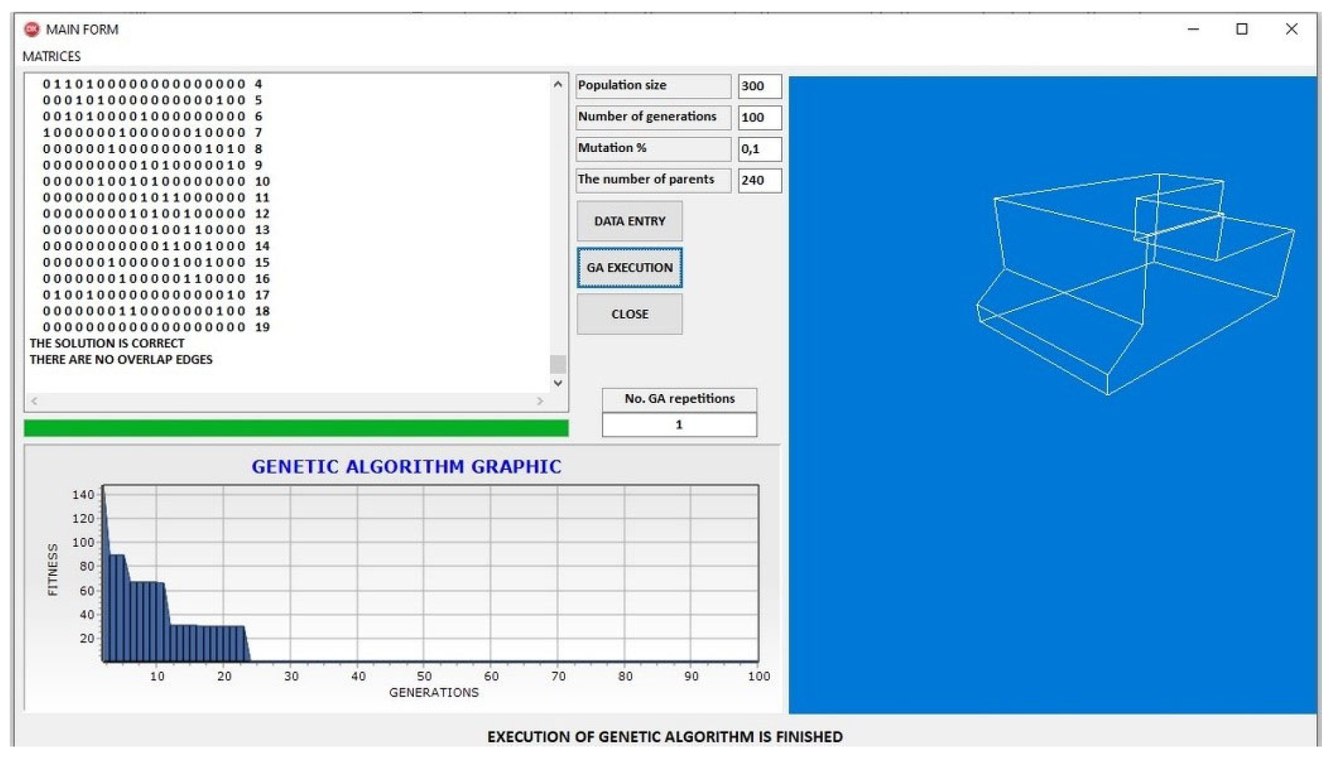
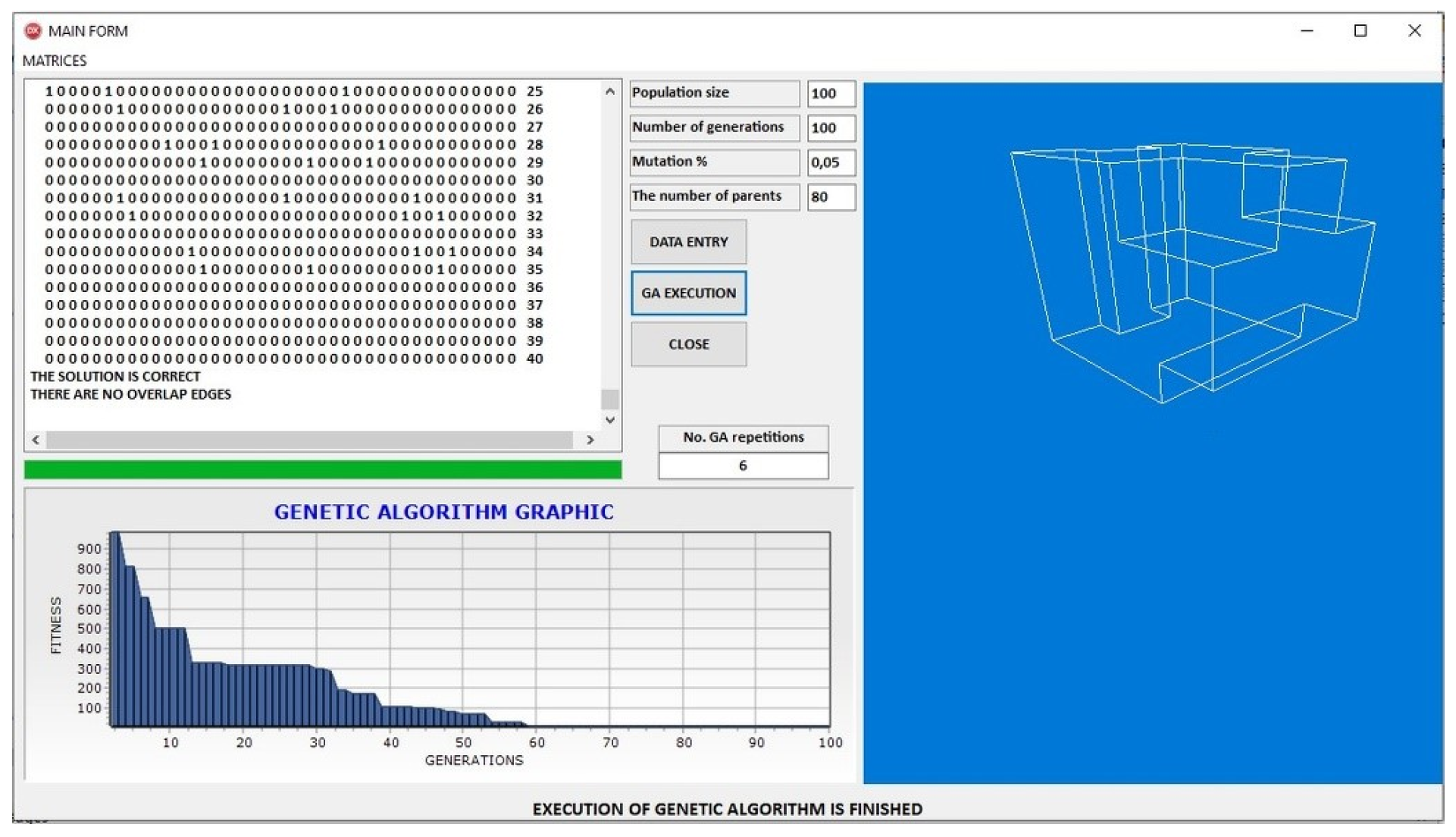
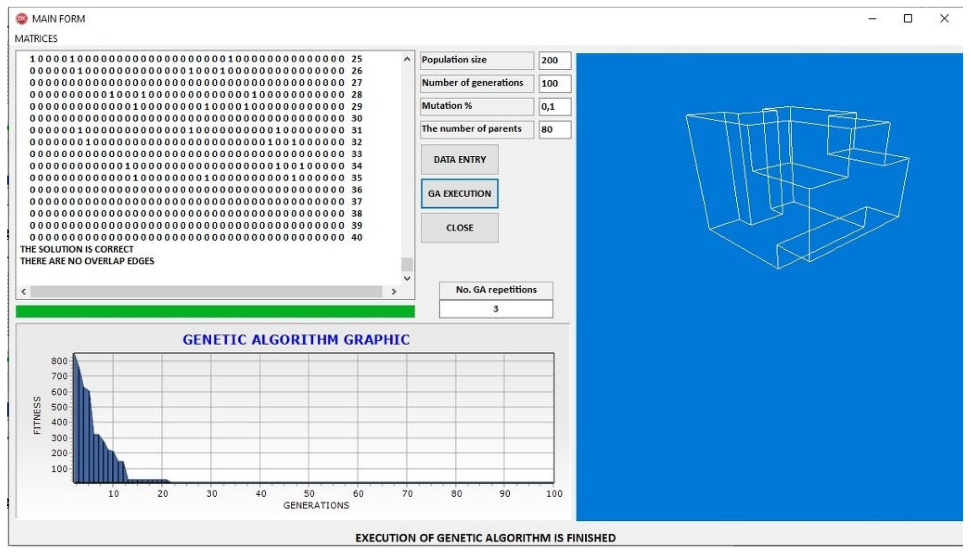
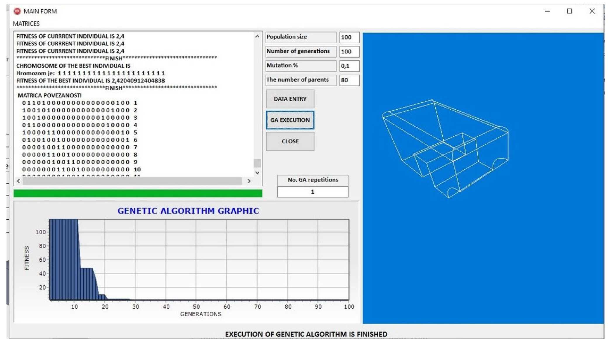
For the simpler polyhedral model PR0003, Figure 11 and Figure 12 depict the GA performance under parameter Groups I and II, respectively. In Figure 11, a steady convergence trend is observed, with gradual fitness improvements stabilizing after approximately 50 generations. The resulting wireframe model adheres to the expected topological structure, demonstrating that even conservative parameter settings can yield valid results. In contrast, Figure 12 reveals a steeper initial drop in fitness values under Group II, indicating faster convergence. Despite the more aggressive parameter configuration, the final model remains both geometrically and topologically consistent, confirming the robustness of the GA framework in lower-complexity scenarios.

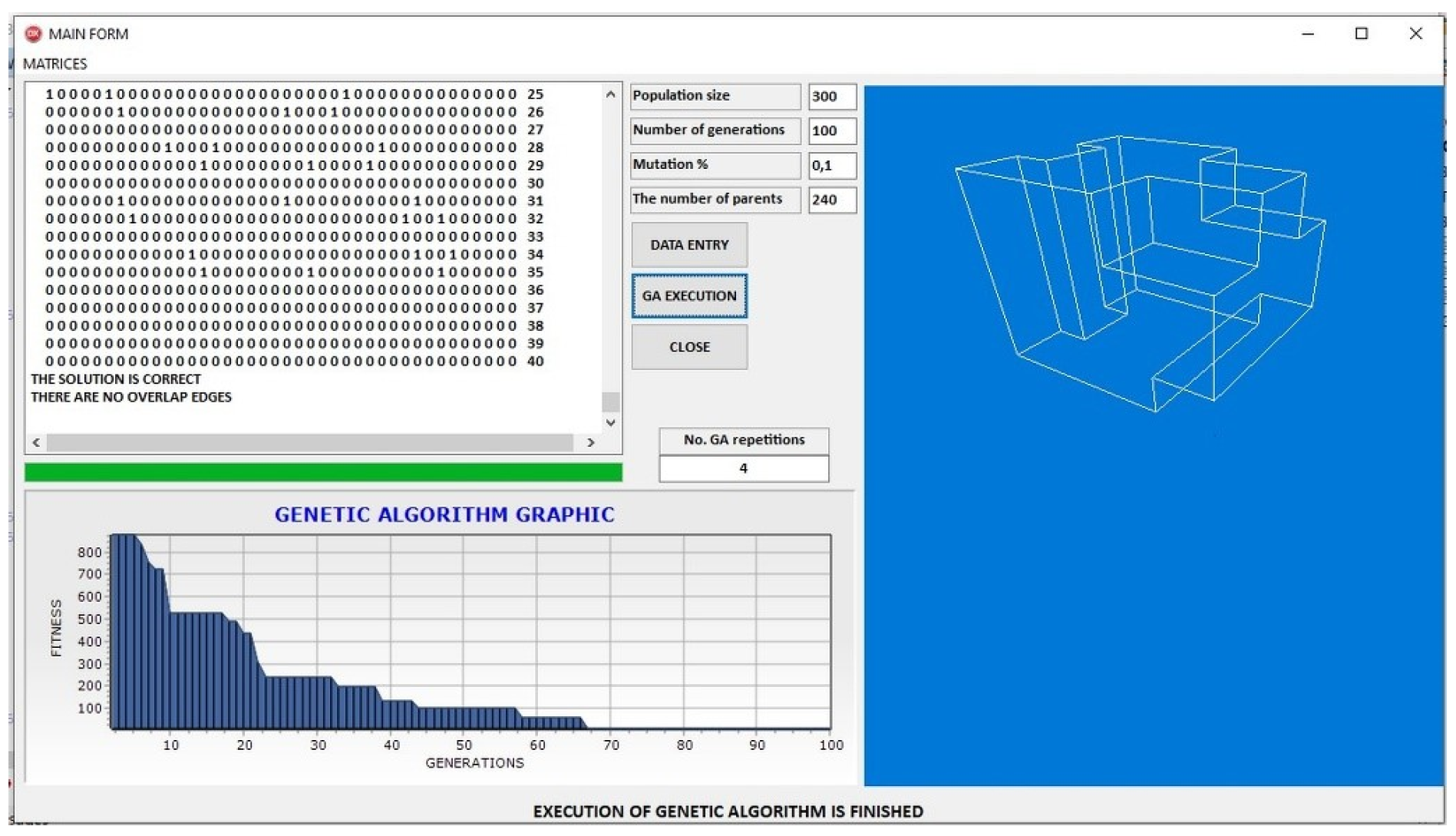
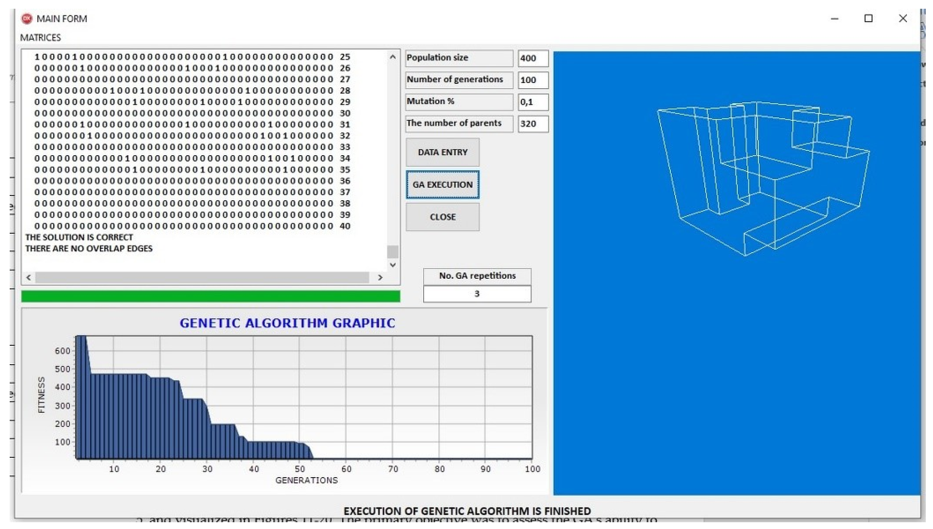
Further testing with Groups III and IV for PR0003, shown in Figure 13 and Figure 14, reveals subtle yet meaningful differences in convergence dynamics. Figure 13 demonstrates that Group III supports rapid early-stage exploration followed by stable convergence, producing a structurally correct wireframe representation. Figure 14, using Group IV, leads to slightly faster convergence, suggesting that fine-tuned parameter values can improve efficiency without compromising solution quality. These results emphasize the importance of parameter calibration, even when dealing with relatively simple geometric forms.

The evaluation is extended to the more complex polyhedral model PR0004, where the algorithm’s scalability is tested against increased topological density and geometric intricacy. In Figure 15, which corresponds to Group I, the convergence curve progresses more gradually, with fitness values improving steadily over time. The adjacency matrix and final model visualization confirm the algorithm’s ability to resolve denser connectivity patterns. Figure 16, representing Group II, shows a more aggressive convergence profile, with earlier stabilization of fitness values and successful reconstruction of the intended 3D geometry, underscoring the algorithm’s adaptability to different optimization pressures.

Figure 17 and Figure 18 offer insight into the GA’s behavior under Groups III and IV for the PR0004 case. Figure 17 illustrates a longer convergence trajectory, with fitness improvements extending across 80 generations, a reflection of the search space complexity. Nonetheless, the final model is both topologically complete and geometrically accurate. Figure 18 isolates the final reconstruction obtained with Group IV and clearly displays the fidelity of the solution, even without the accompanying convergence plot. The preservation of structural proportions across all model layers attests to the reliability of the topological encoding and optimization procedure.

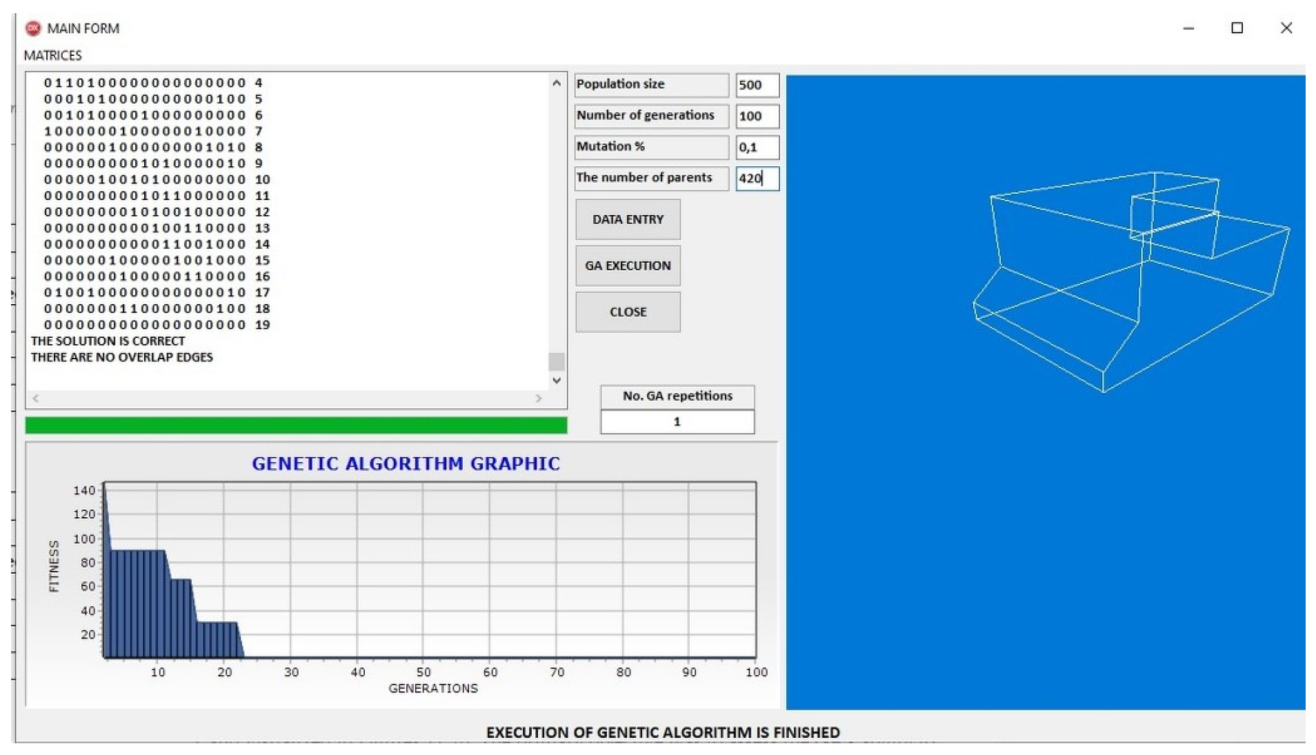
Finally, the outcomes associated with Group V and the fully reconstructed model are presented in Figure 19 and Figure 20. As shown in Figure 19, the algorithm exhibits continued fitness refinement across an extended number of generations, suggesting a broader exploration phase. Despite the higher number of iterations, the resulting solution remains robust, validating the algorithm’s effectiveness even under more exhaustive parameter regimes. Figure 20 displays the final reconstructed geometry in isolation, emphasizing the GA’s capacity to capture the full complexity of the PR0004 model and maintain structural integrity throughout the optimization process.

Collectively, these figures provide strong empirical evidence of the proposed method’s generalizability and resilience across a wide range of parameter settings and model complexities. The consistent convergence behavior and reliable reconstruction outcomes reinforce the applicability of the GA framework to real-world CAD and reverse engineering tasks involving polyhedral geometry.

In the subsequent phase of the experimental evaluation, the focus shifts toward more complex models that incorporate curved surfaces and a combination of cylindrical and rectangular geometries. The objective of this testing stage was to assess the genetic algorithm’s (GA) ability to reconstruct 3D wireframe models for shapes that deviate significantly from purely polyhedral forms. These cases increase the reconstruction challenge and provide insight into the algorithm’s suitability for real-world industrial applications.

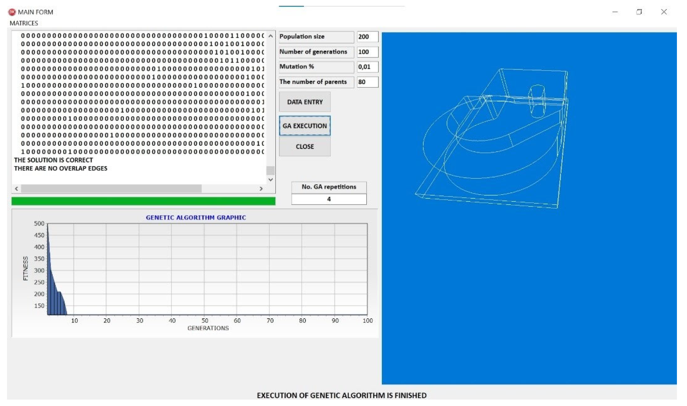
Figure 21 presents the 3D solid model of the PR0007 test case, which features a blend of straight edges, rounded transitions, and a characteristic cutout at the base. This geometry introduces a reconstruction challenge due to the need to preserve topological consistency in the presence of local curvature and interrupted surfaces.

The execution of the GA for PR0007 is shown in Figure 22, where the convergence curve demonstrates rapid early-stage fitness improvement, followed by stabilization. The reconstructed wireframe model faithfully reproduces the primary geometric and topological features of the target object, confirming that the proposed algorithm can handle curved features without relying on additional heuristics.

Moving forward, Figure 23 depicts a more demanding 3D solid model, designated PR0005, which includes complex curved contours, multi-layered structures, and non-rotational symmetries. This model was specifically chosen for its resemblance to real-world components commonly found in mechatronic and precision mechanical assemblies.

The results of applying the GA to PR0005 are illustrated in Figure 24, where the algorithm successfully identifies key edge connections and generates a valid topological mesh. Despite the model’s intricate morphology, the reconstruction maintains geometric consistency, and the convergence curve indicates that the solution is reached within a reasonable number of generations. This confirms the method’s applicability to technically challenging components within engineering environments.

Overall, the visual and quantitative results presented in Figure 11, Figure 12, Figure 13, Figure 14, Figure 15, Figure 16, Figure 17, Figure 18, Figure 19, Figure 20, Figure 21, Figure 22, Figure 23 and Figure 24 confirm the effectiveness and versatility of the proposed GA-based reconstruction framework across a wide spectrum of geometric complexities. The method consistently produced topologically valid and geometrically accurate wireframe models, demonstrating strong potential for integration into automated CAD pipelines and reverse engineering workflows in both academic and industrial contexts.

5. Discussion

The experimental results demonstrate that the GA is highly effective in solving problems involving simple geometries such as PR0003 and also PR0007 with cylindrical surfaces. Even under the most constrained parameter settings, the algorithm consistently converged to the correct solution within a few iterations. For instance, for the PR0003 model, the GA found the exact solution in just two seconds. The same applies to PR0007, which is a part with relatively simple cylindrical surface geometry.

During the testing of other models, it was noticed that this GA is very effective for the models with a number of vertices between 15 and 25 and with a number of edges between 20 and 35. In these intervals, the GA converges to the accurate solution in a single run. During testing mutation was always at 10% rate. Since the results for PR0003 did not change, testing with parameter group V was deemed unnecessary. For more complex parts, such as PR0004, it is clear that an accurate solution is always obtained, but across several runs, which leads to an increased runtime.

The execution time of the GA for complex parts is longer, which also depends on the amount of computation, but this is not a problem regarding the characteristics of modern computers. For example, for PR0004, the ADj matrix is 40 × 40, and intensive calculations are performed on it at all times. In this case, as well as in other more complex parts that were tested, for the number of l vertices greater than 25, solutions are always obtained where the geometric consistency is not violated and the solution does not go beyond the set of solutions represented by the pseudo-wireframe model. Also, no new surfaces are created, and there is no edge overlapping, meaning that individual candidate vertices remain in the solution because all constraints are satisfied and they do not create new shapes in the model.

For typical industrial parts with cylindrical shape, such as the component shown in Figure 23, the execution time is observed to be longer. However, the correct solution is obtained after several GA iterations. This demonstrates that the proposed method effectively handles both simpler and more complex models with cylindrical surfaces.

It should be noted that even the variation of mutation did not lead to convergence to the exact solution, which is also the nature of GA, while for simpler models it converges very quickly to the exact solution because the search space is smaller.

Considering the test results presented in Table 5, Table 6 and Table 7, and the relationship between the complexity of the part being reconstructed and the GA’s execution time, where this time encompasses all GA executions until a valid solution is obtained, it is clear that the proposed GA is most efficient with the second group of parameters for simple and moderately complex geometry parts. During intensive testing of the proposed algorithm, it was also shown that for highly complex geometry parts, the best parameters are from groups IV and V. In all tests conducted to date, the geometry of the part has been consistently and accurately recognized, even for complex components; however, the number of GA executions reached up to eight times, with execution times extending up to 180 s. Given that an accurate solution was consistently obtained, this represents an exceptionally favorable final testing outcome.

In contrast to previous GA-based approaches—which typically rely on raster preprocessing or predefined libraries of geometric primitives—the proposed method employs a mathematically rigorous topological framework that supports the reconstruction of a broader range of 3D models, including those containing curved and free-form elements. By leveraging a connectivity-based representation rather than heuristic feature extraction, the approach enhances model generality and eliminates dependence on prior shape classification. As summarized in

Table 10. Comparison with GA-based 3D reconstruction methods.

Study	Input Type	Shape Support	Method Basis	Optimization Target	Geometry Type Independence	DXF (Vector) Support	Topological Model
Chen & Feng [15]	Raster image	Prismatic + curved	Contour extraction	Projection consistency	✓ Yes	No	Full
Gorgani & Pak [6]	2D drawings	Only prismatic shapes	B-Rep reconstruction	Face alignment	No	No	Partial
Siddique & Zakaria [17]	Raster image	Simple shapes	Shape features	Edge position, face equalization	No	No	No
This paper	DXF (vector)	Prismatic + Curved	Symmetric matrices	Vertex to Vertex–edge topology	Yes	Yes	Full

, this results in improved scalability, increased robustness across diverse input data, and a significant reduction in preprocessing complexity.

Although some of the limitations of the proposed methodology were briefly outlined in Section 3.1, they are revisited and elaborated here to ensure clarity and completeness. This dedicated discussion aims to contextualize the current scope of the model and highlight avenues for future enhancement.

First, the method assumes that the input 2D engineering drawing is complete and composed of exactly three orthographic projections—front, top, and left—conforming to the ISO-E (European) projection standard, as illustrated in Figure 2. These views are expected to encapsulate all essential geometric information, including both visible and hidden edges. At the present stage, the framework does not support sectional views, auxiliary projections, or drawings that are incomplete.

Second, the approach presumes that all orthographic views are rendered at a consistent 1:1 scale, thereby enabling the direct use of vertex coordinates for 3D reconstruction. A global scaling factor may be optionally applied, but the model does not yet incorporate dimensioning metadata or tolerancing information embedded in annotations.

Third, although DXF files are advantageous for extracting basic geometric entities such as lines and arcs, they lack topological information—i.e., they do not provide an explicit mapping of entity connectivity or view separation. Therefore, a custom segmentation procedure is required to distinguish between projections and reconstruct their internal structure.

Additionally, the method relies on the recognition of basic geometric primitives (e.g., LINE, ARC) to infer edge shapes. In its current form, the model does not support complex freeform surfaces or non-cylindrical geometries. Interpretation of such features would require integrating advanced geometric representations and curvature analysis tools and mathematical tools for curvature and surface analysis.

It is important to emphasize that these constraints do not compromise the core of the methodology, which is fundamentally based on a binary vertex-to-vertex topological model. The approach remains general and extensible, and these limitations may be addressed through future enhancements, such as the incorporation of geometric reasoning modules or hybrid shape descriptors. Therefore, the challenges identified here also represent promising directions for future research and model refinement.

6. Conclusions

In this paper, a method for encoding 2D engineering drawings using symmetric connectivity matrices is presented. These matrices significantly facilitate the formation of a mathematical model and enable the problem of recognizing 3D models from 2D engineering drawings to be reduced to an integer linear programming problem. A GA has been developed, successfully recognizing 3D models of both polyhedral shapes and models with cylindrical surfaces. For testing purposes, a fully independent software platform was created, covering the entire process from generating symmetric adjacency matrices from orthogonal projections to part recognition. This platform includes real-time graphical visualization of the recognition process and allows testing of parts with various geometric shapes without additional adjustments.

The advantage of the proposed model lies in its simplicity, as the problem of recognizing a 3D wireframe model is reduced to the problem of linear integer programming. The model does not necessarily require a DXF format as a starting point, as it is designed to accept, with minor modifications, any other vector format used for engineering drawings. So far, it has only been tested on polyhedral shapes, and on simpler cylindrical ones, although theoretically, it should also work with all shapes since it is based on edges, including curved edges that are not straight lines.

To the best of our knowledge, no previous work in the available literature has introduced a 3D reconstruction model that combines symmetric connectivity matrices with GA. Furthermore, studies [16,17,18,19] that utilize GA for geometry recognition generally achieve lower success rates in 3D reconstruction and are predominantly limited to polyhedral shapes.

However, one of its shortcomings is that it does not recognize surfaces but only the wireframe model, and has not yet been tested on parts with highly complex geometry, which, in addition to polyhedral shapes and cylindrical surfaces, also include other types of surfaces.

Future research directions involve improving the GA process, potentially selecting other crossover and mutation operators, redefining weight coefficients and methods for penalizing poor individuals, and possibly hybridizing GA with other optimization algorithms to achieve even better results with polyhedral shapes and cylindrical surfaces. Additionally, intensive testing and possible modifications are required to recognize other non-cylindrical surfaces.

This solution, as conceived, can serve as a foundation for the complete automation of the 3D model recognition process from engineering drawings, or as an initial phase toward the full integration of CAD/CAM activities.

In future work, we aim to expand the proposed methodology beyond wireframe reconstruction, with the goal of achieving fully automated generation of solid models directly from standard technical documentation. This advancement would facilitate the practical integration of the method into industrial CAD environments, thereby enhancing its applicability in real-world engineering workflows.

Moreover, the utilization of symmetric adjacency matrices establishes a geometry-independent framework that enables the method to process both linear and nonlinear edges with equal robustness. By prioritizing topological relationships over explicit surface definitions, the approach circumvents limitations commonly associated with specific part geometries. This abstraction not only improves the generalizability of the system but also creates opportunities for further extension into complex design domains, including freeform surfaces and non-standard projection views. Such developments would significantly broaden the scope of the method and reinforce its relevance in advanced CAD and reverse engineering applications.