Automated Eye Disease Diagnosis Using a 2D CNN with Grad-CAM: High-Accuracy Detection of Retinal Asymmetries for Multiclass Classification

Abstract

Eye diseases (EDs), including glaucoma, diabetic retinopathy, and cataracts, are major contributors to vision loss and reduced quality of life worldwide. These conditions not only affect millions of individuals but also impose a significant burden on global healthcare systems. As the population ages and lifestyle changes increase the prevalence of conditions like diabetes, the incidence of EDs is expected to rise, further straining diagnostic and treatment resources. Timely and accurate diagnosis is critical for effective management and prevention of vision loss, as early intervention can significantly slow disease progression and improve patient outcomes. However, traditional diagnostic methods rely heavily on manual analysis of fundus imaging, which is labor-intensive, time-consuming, and subject to human error. This underscores the urgent need for automated, efficient, and accurate diagnostic systems that can handle the growing demand while maintaining high diagnostic standards. Current approaches, while advancing, still face challenges such as inefficiency, susceptibility to errors, and limited ability to detect subtle retinal asymmetries, which are critical early indicators of disease. Effective solutions must address these issues while ensuring high accuracy, interpretability, and scalability. This research introduces a 2D single-channel convolutional neural network (CNN) based on ResNet101-V2 architecture. The model integrates gradient-weighted class activation mapping (Grad-CAM) to highlight retinal asymmetries linked to EDs, thereby enhancing interpretability and detection precision. Evaluated on retinal Optical Coherence Tomography (OCT) datasets for multiclass classification tasks, the model demonstrated exceptional performance, achieving accuracy rates of 99.90% for four-class tasks and 99.27% for eight-class tasks. By leveraging patterns of retinal symmetry and asymmetry, the proposed model improves early detection and simplifies the diagnostic workflow, offering a promising advancement in the field of automated eye disease diagnosis.

1. Introduction

The human eye is a remarkable and indispensable organ that plays a vital role in our daily lives. It is the most relied upon of the five senses and it processes over 80% of external information through the sense of sight. Vision, the dominant sense in humans, allows us to perceive the world in vibrant color, distinct shapes, fluid motion, and depth. This sensory ability accounts for approximately 80% of the information we gather from our surroundings, enabling us to interact with and navigate through our environment effectively. From the simple pleasures of appreciating nature’s beauty to the complex tasks of reading, driving, and recognizing faces, our daily activities are heavily reliant on the function of our eyes [1].

Vision is not only essential for our routine endeavors but also plays a critical role in identifying potential dangers and avoiding risks. Whether it is detecting an approaching object, navigating uneven terrain, or reading warning signs, our eyes empower us to respond quickly and safely to threats, aiding in our overall survival. Moreover, the eye provides us with spatial awareness and coordination, allowing us to carry out tasks efficiently and effectively. Eyes are also a vital component of non-verbal communication, as eye contact, movement, and expressions convey a range of emotions, from happiness and sadness to anger and confusion. These visual cues are integral to our social interactions and relationships. Overall, the eye is an indispensable organ, essential for our functioning, safety, learning, and emotional balance. Its importance in human life cannot be overstated, as it enables us to perceive and engage with the world around us in profound and meaningful ways [2,3].

EDs refer to any condition or illness that impairs the eye’s ability to function properly or adversely affects the eye’s visual acuity. Fundus disorders as depicted in Figure 1 are the primary cause of blindness in humans. Some of the most common ocular illnesses include [4]:

• Diabetic Macular Edema (DEM): Diabetic damage to the blood vessels in the retina leads to this condition. It particularly impacts the macula, which is the central region of the retina that is crucial for clear and detailed vision.
• Choroidal Neovascularization (CNV): It is characterized by the formation of irregular blood vessels originating from the choroid, which is the blood-rich layer located beneath the retina, and extending into the retinal layers. This condition can result in considerable vision impairment caused by the leakage of blood or fluid, as well as scaring and harm to the structure of the retina.
• Drusen: They are yellowish substances that accumulate under the retina, located specifically between the retinal pigment epithelium (RPE) and Bruch’s membrane. Although small quantities of drusen are a typical aspect of the aging process, their existence and features may suggest specific retinal conditions, especially age-related macular degeneration (AMD).

It is important to seek medical attention and treatment to manage these conditions and prevent further vision impairment. EDs can cause permanent damage to the retina, which is the light-sensitive tissue at the back of the eye [5]. This eye damage may result in visual impairment or even blindness, making it challenging for individuals to perform everyday tasks such as reading, driving, recognizing faces, and navigating their surroundings [5]. Consequently, visual impairment can significantly impact an individual’s quality of life. Globally, at least 2.2 billion people are experiencing some form of visual impairment [5]. This includes 88.4 million individuals with moderate or severe distance vision impairment or blindness due to unaddressed refractive error, 94 million people with cataract, 8 million individuals with age-related macular degeneration, 7.7 million people affected by glaucoma, 3.9 million individuals with diabetic retinopathy, and 826 million people with near vision impairment caused by unaddressed presbyopia [5,6]. The global economic burden of vision impairment is estimated at 411 billion USD annually, representing a substantial strain on economies worldwide [5]. According to the latest estimates, the global population of individuals with vision impairments is projected to reach approximately 285 million. Within this figure, 39 million people are classified as legally blind, while an additional 246 million are considered to have some degree of impaired vision [5,7].

The prevalence of eye diseases varies significantly across the globe, influenced by a range of factors such as age, gender, occupation, lifestyle, economic status, hygiene, customs, and environmental conditions. A comparative study of tropical and temperate regions reveals that tropical populations tend to have a higher incidence of stubborn eye infections. This is largely attributed to the presence of natural elements like dust, humidity, and sunlight, which are more prevalent in tropical climates and can contribute to the increased occurrence of these eye health issues [8]. Between emerging and developed countries, eye illnesses manifest differently within communities. In less industrialized nations, especially in Asia, there are high levels of visual impairments that often go undetected and untreated [9].

Children with intense visual impairment may encounter delays in various developmental areas, such as motor, verbal, emotional, social, and cognitive domains [10,11,12,13]. Low academic achievement is a common challenge for school-aged children with visual impairments. Conventional treatment approaches for conditions like dry eye, conjunctivitis, and blepharitis have often fallen short in providing a comprehensive solution for visual impairment. These standard methods have been known to cause discomfort and pain for patients [14]. The primary goal in managing these disorders is to alleviate symptoms and prevent the worsening of the underlying condition. However, the limitations of traditional treatments have highlighted the need for alternative and more effective strategies to address visual impairment.

Vision rehabilitation has demonstrated remarkable effectiveness in enhancing the functionality and overall quality of life for individuals grappling with permanent vision impairment stemming from diverse eye conditions. This comprehensive approach encompasses a wide range of eye-related disorders, including diabetic retinopathy (DR), glaucoma, vision impairment resulting from trauma, and age-related macular degeneration. Through tailored interventions and assistive technologies, vision rehabilitation empowers those affected by vision loss, equipping them with the means to regain independence, adapt to their evolving visual needs, and bolster their performance in everyday activities [15].

Medical imaging refers to a diverse range of technologies that produce visual representations of the body’s internal structures [16]. These visual tools are essential for conducting non-invasive assessments of anatomical characteristics and physiological processes [17]. Healthcare professionals rely on these images to identify, monitor, and manage various health issues. However, they also have certain constraints such as [17]:

• Restricted Visual Information: Certain medical imaging techniques, like fundus photography or OCT, may have difficulty capturing highly detailed information, particularly in the early stages of eye conditions. This can lead to missed diagnoses or delayed identification of subtle changes in the retina or optic nerve. Early-stage diseases, such as glaucoma or DR, may be challenging to detect due to resolution limitations, potentially delaying necessary treatment.
• Reliance on Expert Interpretation: The accurate identification of EDs through medical imaging often relies heavily on the expertise and experience of healthcare professionals analyzing the images. Misinterpretation or insufficient experience can lead to inaccurate diagnoses or delayed treatment. The most advanced imaging technologies are susceptible to human error, especially when differentiating between conditions with similar visual characteristics.
• False Positives/Negatives: Medical imaging can sometimes produce false positive results, which indicate the presence of a disease when none exists. Conversely, false negative results may fail to detect an existing disease. These inaccuracies can have significant consequences. False positives can lead to unnecessary medical treatments, while false negatives may result in missed interventions. Ultimately, misdiagnosis based on imaging results can cause psychological distress for patients and lead to inadequate or inappropriate treatment plans.
• Challenges with Detecting Certain Disease Aspects: Some eye conditions, such as early macular degeneration or mild optic neuropathy, may not display clear symptoms in medical images during their initial stages. Additionally, certain diseases can affect parts of the eye that are challenging to visualize using standard imaging techniques. This can result in delayed diagnosis and treatment until the disease has advanced further, potentially leading to irreversible damage.
• Availability and Cost: Advanced imaging technologies like OCT, magnetic resonance imaging (MRI), or fluorescein angiography can be expensive and may not be available in all healthcare settings, particularly in low-resource areas. Access to high-quality imaging may also be limited by economic constraints or the availability of equipment and skilled personnel. Lack of access to advanced imaging can delay or limit the proper diagnosis and management of eye diseases in certain populations.

To address these challenges, the integration of artificial intelligence (AI) into the medical field has been steadily increasing. AI-based tools and technologies are leveraged to empower healthcare centers to more effectively detect EDs [18]. These systems utilize advanced DL algorithms to analyze medical images and identify potential signs of EDs with greater consistency and precision than human experts [19]. Through CAD systems, healthcare providers can benefit from more reliable and timely diagnoses, ultimately leading to improved patient outcomes and more effective treatment interventions. The integration of automated detection into the clinical workflow can significantly enhance the efficiency and effectiveness of ED identification. These systems can rapidly process large volumes of medical images, screening for potential indicators of EDs and flagging cases that require further investigation by healthcare professionals. This can result in earlier detection, faster treatment initiation, and better long-term prognosis for individuals suffering from these conditions [20].

Furthermore, automated detection systems can be trained on extensive datasets, enabling them to recognize subtle patterns and nuances that may be difficult for human experts to detect. By continuously learning and refining their algorithms, these systems can become increasingly accurate and reliable over time, providing a valuable tool for healthcare providers in the fight against EDs [19].

DL, a subset of machine learning (ML), is extensively applied in AI systems [21]. Convolutional neural networks (CNNs) are particularly effective for automatic feature extraction and learning kernels to analyze images within small perceptual areas, and they reduce computational complexity [22,23]. Unlike fully connected neural networks, CNNs can train and reuse filter weights, enhancing efficiency. This allows for the creation of deeper networks capable of handling more complex tasks. The perceptual fields in CNNs enhance capabilities like image recognition, classification, and clinical diagnosis by identifying high-level features such as texture, structure, and gradients [14].

This paper builds a 2D single-channel CNN using ResNet101-V2 to leverage the capabilities of DNNs for detecting EDs. Additionally, the proposed model employs the Grad-CAM technique to identify specific areas affected by GGOs associated with EDs. This model enhances the early detection of EDs, allowing for timely intervention and improved patient outcomes, while also streamlining the diagnostic process to minimize time and costs for patients. We conducted two experiments using the two OCT datasets for multiclass classification tasks, with four and eight classes. The data underwent pre-processing through techniques such as data augmentation, resizing, and normalization to ensure uniform input. Our proposed DL model was compared against traditional classifiers. The contributions of the research are summarized below:

• A robust, fine-tuned, customized deep ResNet101-V2 (CDResNet101-V2) model was proposed to predict EDs based on ResNet101-V2 through the OCT4 and OCT8 datasets.
• We performed a comprehensive experiment utilizing two OCT datasets, incorporating Grad-CAM to analyze the model’s decisions and offering visual explanations.
• We compared the proposed fine-tuned model to more recent CNN models for a highly accurate multiclassification, such as EfficientNet-B3, DenseNet201, InceptionV3, MobileNet-V2, and VGG16.
• The proposed fine-tuned model presented in this research demonstrated the ability to detect EDs with high accuracy and efficiency. This innovative approach can greatly assist pathologists in the early identification of EDs, enabling timely and appropriate treatment for patients.
• For the four-class classification task, the proposed model achieved an accuracy of 99.90%, specificity of 99.93%, precision of 99.80%, recall of 99.79%, and F1-score of 99.79%. In the eight-class classification task, the model attained an accuracy of 99.27%, specificity of 99.58%, precision of 97.13%, recall of 97.10%, and F1-score of 97.10%.

The remainder structure of this paper is as follows: Section 2 provides a review of the literature on ED diagnostic systems. Section 3 outlines the pre-processing procedures for the ODIR dataset, as well as the methodology of the proposed model. The experimental results of the proposed framework are detailed in Section 4, and the conclusion is presented in Section 5.

2. Literature Review

ED diagnosis has emerged as a prominent research focus in the field of medical image analysis. Numerous studies have addressed this challenge from diverse perspectives. Researchers are actively exploring various approaches to enhance the understanding and identification of EDs through the analysis of medical imagery. For example, Baba, S. et al. [24] concentrated on using OCT images to identify macular disorders commonly related to aging. They created a specialized CNN model to classify OCT images into four categories: normal, CNV, DME, and drusen, utilizing the publicly available OCT dataset. The authors conducted experiments to evaluate the effectiveness of their proposed model in comparison to traditional ML techniques and other transfer learning models. The results showed that the proposed model performed well, achieving a testing accuracy of 98%.

Quek, T.C. et al. [25] developed a segmentation DL network that combined a CNN with a Vision Transformer (ViT), trained on a small dataset of 100 training images (which were augmented to 992 images) from the Singapore Epidemiology of Eye Diseases (SEED) study. This was paired with a CNN-based classification network trained on 8497 images, capable of distinguishing between fluid and non-fluid OCT scans. Both networks were validated using external datasets. The proposed segmentation network achieved an internal testing Intersection over Union (IoU) score of 83.0% (95% confidence interval (CI) = 76.7–89.3%) and a DICE score of 90.4% (86.3–94.4%). For external testing, the IoU score was 66.7% (63.5–70.0%), and the DICE score was 78.7% (76.0–81.4%). In internal testing, the classification network produced an area under the receiver operating characteristics curve (AUC) of 99.18% and a Youden index threshold of 0.3806. During external testing, it achieved an AUC of 94.55%, with an accuracy of 94.98% and an F1-score of 85.73% along with the Youden index.

Elkholy, M. et al. [26] proposed a DL algorithm that detected three different diseases by extracting features from OCT images. The DL algorithm employed a CNN to classify OCT images into four categories: normal retina, DME, choroidal neovascularization (CNM), and age-related macular degeneration (AMD). The study utilized publicly available OCT retinal images as its dataset. The experimental results demonstrated a significant improvement in classification accuracy, achieving 97% while detecting features of the three specified diseases.

Wu, J. et al. [27] proposed the Retinal Layer Macular Edema Network (RLMENet) model, which aimed to perform the end-to-end joint segmentation of retinal layers and fluids. This network utilized dense multiscale attention to enhance the extraction of detailed information regarding retinal layers and fluids. It achieved efficient long-range modeling, thereby improving the receptive field and obtaining multiscale features. The design of a more complex decoder allowed for the integration of additional low-level feature information, which facilitated the extraction of more features. This process gradually restored the resolution of the feature map and increased segmentation accuracy. Wu, J. et al. utilized a portion of the OCT dataset for training and validating the model, dividing the data into a training set, validation set, and test set in a 7:2:1 ratio. They also evaluated the proposed method on the ISIC2017 dataset. The experimental results indicated that the RLMENet model could accurately segment seven retinal tissue layers and diabetic macular edema (DME) lesions within the retinal OCT dataset. Ultimately, the mean Intersection over Union (MIoU) value achieved in the test set was 86.55%.

Tsuji, T. et al. [28] created a training set consisting of 83,484 images and a test set with 1000 images from the OCT dataset. The training set included 37,205 images showing CNV, 11,348 images with DME, 8616 images featuring drusen, and 26,315 normal images. The test set contained 250 images from each category. The model developed utilized a capsule network to enhance classification accuracy and was trained using the training set. After training, the test set was employed to assess the model’s performance. The proposed method for classifying OCT images achieved an impressive accuracy rate of 99.6%.

He, J. et al. [29] introduced an interpretable Swin-Poly Transformer network designed for the automatic classification of retinal OCT images. By adjusting the window partitioning, the Swin-Poly Transformer established connections between adjacent non-overlapping windows from the previous layer, allowing for greater flexibility in modeling multiscale features. Additionally, this transformer adjusted the significance of polynomial bases to enhance cross-entropy, leading to improved classification of retinal OCT images. The proposed method also generated confidence score maps, which help medical practitioners comprehend the decision-making process of the models. Experiments conducted on the OCT-2017 and OCT-C8 datasets demonstrated that the proposed method exceeded the performance of both CNN and ViT approaches, achieving an accuracy of 99.80% and an AUC of 99.99%.

Hassan, E. et al. [30] proposed an Enhanced Optical Coherence Tomography (EOCT) model for classifying retinal OCT images using modified ResNet (50) and Random Forest (RF) algorithms. These algorithms were incorporated into the training strategy of the study to improve performance. The Adam optimizer was utilized during the training process to enhance the efficiency of the ResNet (50) model when compared to commonly used pre-trained models like Spatial Separable Convolutions and Visual Geometry Group (VGG) (16). The experimental results demonstrated the following metrics: sensitivity of 0.9836, specificity of 0.9615, precision of 0.9740, negative predictive value of 0.9756, false discovery rate of 0.0385, false negative rate (FNR) of 0.0260, accuracy of 0.9747, and Matthew’s correlation coefficient of 0.9474.

Laouarem, A. et al. [31] highlighted that integrating the strengths of CNNs with ViTs presented a promising approach for image processing, significantly improving both robustness and efficiency. The proposed model introduced a hierarchical CNN module called Convolutional Patch and Token Embedding (CPTE). This module replaced the traditional method of directly tokenizing raw OCT images in the transformer. The CPTE module was specifically designed to embed an inductive bias, which reduced reliance on large datasets and addresses the challenges related to low-level feature extraction in ViTs. Recognizing the importance of local lesion details in OCT images, the model also utilized a parallel architecture known as Residual Depthwise–Pointwise ConvNet (RDP-ConvNet) for extracting high-level features. RDP-ConvNet employed depthwise and pointwise convolution layers within a residual network structure. The overall performance of the HTC-Retina model was evaluated using three datasets: OCT-2017, OCT-C8, and OCT-2014. The model outperformed previously established benchmarks, achieving accuracy rates of 99.40%, 97.00%, and 99.77%, along with sensitivity rates of 99.41%, 97.00%, and 99.77%, respectively.

Khalil, I. et al. [32] introduced a new model named OCTNet, which integrates DL techniques by combining InceptionV3 with a modified multiscale attention-based spatial attention block to improve performance. OCTNet leveraged the InceptionV3 framework, enhanced by two attention modules, to construct its architecture. The InceptionV3 model was proficient at extracting intricate features from images, effectively capturing both local and global contexts. The quality of feature extraction was further augmented through the incorporation of the modified multiscale spatial attention block, resulting in a significant improvement in the quality of the feature map. To evaluate the model’s performance, authors used two advanced datasets containing images of various conditions, including normal cases, CNV, drusen, and DME. Through extensive experimentation and simulations, Khalil, I. et al. discovered that the proposed OCTNet improved the classification accuracy of the InceptionV3 model by 1.3%, outperforming other leading models. The model achieved overall average accuracies of 99.50% and 99.65% across two distinct OCT datasets.

Table 1. Summary of state of the art.

Reference	Methodology	Evaluation Metrics	Advantages	Limitation
Baba, S. et al. [24]	CNN	Accuracy: 98%	Custom-designed CNN architecture specifically optimized for retinal disease classification using OCT images	Lack of external validation and potential overfitting
Quek, T.C. et al. [25]	CNN-ViT	Accuracy: 94.98%	High segmentation performance on internal data	Small segmentation training set and external performance degradation
Elkholy, M. et al. [26]	CNN and VGG16	Accuracy: 97%	Application of CNNs for feature extraction	Lack of detailed performance metrics and potential overfitting concerns
Wu, J. et al. [27]	RLMENet	MIoU of 86.55% and an MPA of 98.73%.	Joint end-to-end segmentation and dense multiscale attention	Limited public OCT training data, computational complexity, and potential domain shift
Tsuji, T. et al. [28]	Capsule network	Accuracy: 99.6%	Preserves spatial/positional relationships, shallower architecture, and fewer parameters	Potential class imbalance and dataset bias and computational overhead of dynamic routing
He, J. et al. [29]	Swin-Poly Transformer network	Accuracy: 99.80%	Multiscale feature modeling via shifted windows and improved loss optimization with PolyLoss	Computational complexity and resource demands; potential overfitting to dataset biases
Hassan, E. et al. [30]	ResNet (50) and RF algorithms	Accuracy: 97.47%	Dual-optimizer training yields faster convergence and hybrid architecture leverages CNN feature extraction + ensemble robustness	Requirement for large, diverse training data; small validation set raises robustness concerns; computational and memory demands
Laouarem, A. et al. [31]	CPTE	Accuracy: 99.40%	Captures both local and global features, reduces reliance in massive, annotated datasets, and maintains computational efficiency	Difficulty with tiny or subtle lesions, confusion between visually similar disease patterns, and limited interpretability
Khalil, I. et al. [32]	OCTNet	Accuracy: 99.50%	Multiscale feature representation, dual attention fusion, and ablation-verified design choices	Limited dataset variability, potential overfitting on small data, and computational complexity

provides a summary of the above studies, and the limitations of the above research are as follows:

• The researchers referenced earlier focused on metrics like accuracy, precision, recall, and F1-score; however, they neglected to evaluate results through the lens of statistical confidence intervals. In contrast, our approach effectively incorporates statistical methods to analyze and compare outcomes from various DL techniques by investigating confidence intervals. This highlights the distinctive advantage of our methodology.
• The authors of the earlier study did not utilize the Grad-CAM algorithm. On the other hand, we implemented this algorithm to identify specific areas impacted by ground glass opacities (GGOs) that correlate with EDs.
• The authors of the prior research did not perform an ablation study. In contrast, we conducted this study to understand the influence of individual components or features within our proposed model by systematically removing or altering them and assessing the effect on performance.

In this research, we sought to introduce a novel approach for predicting EDs, addressing the shortcomings of existing methods. Our technique utilizes a 2D single-channel CNN that minimizes the potential for errors while avoiding interslice motion and preventing an increase in dimensionality.

3. Materials and Methods

In this section, we outline the origins, sizes, and class distributions of the two datasets used. We also detail the pre-processing steps undertaken for each dataset, the methodology employed, and the proposed model along with the model architectures utilized.

3.1. Materials

OCT-2017 images, specifically from the Spectralis OCT system by Heidelberg Engineering in Germany, were collected from retrospective groups of 4686 adult patients. These patients were sourced from various institutions, including the Shiley Eye Institute at the University of California, San Diego, the California Retinal Research Foundation, Medical Center Ophthalmology Associates, Shanghai First People’s Hospital, and Beijing Tongren Eye Center. The data collection period spanned from 1 July 2013 to 1 March 2017 [4]. Before the training phase, each image went through a comprehensive grading system that involved multiple layers of trained graders with increasing levels of expertise for validation and correction of image labels. Initially, every image added to the database was labeled based on the most recent diagnosis of the patient. The first level of grading involved undergraduate and medical students who had completed an OCT interpretation course. These graders conducted initial quality control, removing OCT images that had severe artifacts or significant reductions in image quality. The second level consisted of four ophthalmologists who independently assessed each image that had successfully passed the first level. They recorded the presence or absence of CNV (whether active or in the form of subretinal fibrosis), macular edema, drusen, and other identifiable pathologies in the OCT scan. Finally, the third level included two senior independent retinal specialists, each with over 20 years of clinical experience in retina, who verified the accuracy of the labels for every image. To prevent data leakage, we conducted patient-level splits so that no patient appears in more than one of the training, validation or test subsets. We further stratified sampling by both disease class and acquisition site to maintain consistent prevalence across splits. To reduce human error in grading, a validation subset of 993 scans was evaluated separately by two ophthalmologist graders, with any discrepancies in clinical labels resolved by a senior retinal specialist [33]. The OCT-2017 dataset consists of 84,484 images in JPEG format, categorized into four groups: normal, CNV, DME, and drusen, as shown in

Table 2. The class distribution of OCT-2017.

Class	Image Count in Training Set	Image Count in Testing Set	Image Count in Validation Set
CNV	37,205	242	8
DME	11,348	242	8
Drusen	8616	242	8
Normal	26,315	242	8
Total	83,484	968	32

and Figure 2. The distribution of the training and test sets is shown in Figure 3 and Figure 4.

The OCT-C8 dataset includes 24,000 images divided into eight different categories: AMD, CNV, central serous retinopathy (CSR), DME, diabetic retinopathy (DR), drusen, macular hole (MH), and normal. Each category contains 2300 images designated for training, 350 for validation, and 350 for testing, as shown in

Table 3. The class distribution of OCT-C8.

Class	Image Count in Training Set	Image Count in Testing Set	Image Count in Validation Set
AMD	2300	350	350
CNV	2300	350	350
CSR	2300	350	350
DME	2300	350	350
DR	2300	350	350
DRUSEN	2300	350	350
MH	2300	350	350
NORMAL	2300	350	350
Total	18,400	2800	2800

and Figure 5. The maximum resolution of the OCT images is 384 × 496 pixels, while the minimum resolution is 1536 × 496 pixels [34].

3.2. Methodology

To detect EDs from images, we developed a model named CDResNet101-V2, which was a 2D single-channel CNN utilizing ResNet101-V2. This model leveraged the capabilities of DNNs specifically for ED detection. Our research concentrated on the initial layers of the ResNet101-V2 model. Additionally, it optimized the diagnostic process with the goal of reducing both time and costs for patients. Furthermore, the proposed model utilized the Grad-CAM technique to pinpoint specific areas impacted by GGOs related to EDs. We conducted two experiments using two OCT datasets for multiclass classification tasks, consisting of four and eight classes, respectively. The data underwent pre-processing methods including data augmentation, resizing, and normalization to ensure consistent input. The architecture of the proposed DL model is illustrated in Figure 6, while Algorithm 1 outlines the algorithm used for fine-tuning the six DL models. The steps of the proposed DL model are detailed as follows:

Phase 1 (Dataset Pre-processing): The two OCT datasets were obtained from Kaggle and prepared during the first phase. In the preparation process, the images of the OCT datasets were resized, augmented, and standardized.

Phase 2 (OCT Splitting): In the second phase, the two OCT datasets were divided into three distinct parts: the training set, the test set, and the validation set. For the OCT-2017 dataset, the training set consisted of 83,484 images, the test set included 968 images, and the validation set contained 32 images. In the case of the OCT-C8 dataset, the training set comprised 18,400 images, while both the test and validation sets had 2800 images each.

Phase 3 (Using 6 Pre-training DL Models): We selected five advanced pre-trained DL models in addition to the CDResNet101-V2 model, all of which were developed using the ImageNet dataset. The chosen models are MobileNet-V2, EfficinetNet-B0, EfficinetNet-B3, NASNetMobile, and ResNet50.

Phase 4 (Fine-tuning for the 6 DL Models): The six DL models were fine-tuned using the training sets of the two OCT datasets to achieve the optimal hyperparameters.

Phase 5 (Multiclassification using the 6 DL Models): The six DL models were employed to carry out multiclass classification on the two OCT datasets. Furthermore, the performance of our proposed DL approach was evaluated using the specified metrics.

Algorithm 1: The fine-tuning algorithm. Fine-tuned CDResNet101-V2, MobileNet-V2, EfficinetNet-B0, EfficinetNet-B3, NASNetMobile, and ResNet50
1	Input$\to$$\mathrm{OCT} 4 D1$$\mathrm{and} \mathrm{OCT} 8 D2$
2	Output$\leftarrow$ Fine-tuned six DL models
3	BEGIN
4	STEP 1: Pre-processing of Images
5	$\mathbf{FOR} \mathbf{EACH} \mathrm{image} \mathbf{IN} \mathrm{the} D1$DO
6	Resize the image to 299 × 299 pixels
7	Normalize pixel values from range [0, 255] to [0, 1]
8	Augmentation
9	END FOR
10	$\mathbf{FOR} \mathbf{EACH} \mathrm{image} \mathbf{IN} \mathrm{the} D2$DO
11	Resize the image to 299 × 299 pixels
12	Normalize pixel values from range [0, 255] to [0, 1]
13	Augmentation
14	END FOR
15	STEP 2: OCT Splitting
16	$\mathbf{SPLIT} D$ and INTO
17	Training set $\to$$98.8\%$ of $D_1$ and 76.8% of $D_2$
18	Testing set $\to$$1.14\%$ of $D_1$ and 11.6% of $D_2$
19	Validation set $\to$$0.03\%$ of $D_1$ and 11.6% of $D_2$
20	STEP 3: Six DL Models Training
21	FOR EACH DL IN [CDResNet101-V2, MobileNet-V2, EfficinetNet-B0, EfficinetNet-B3, NASNetMobile, and ResNet50] DO
22	Load DL model.
23	pre-trained DL on the ImageNet dataset.
24	END FOR
25	STEP 4: Fine-Tuning Six DL Models
26	FOR EACH pre-trained DL IN [CDResNet101-V2, MobileNet-V2, EfficinetNet-B0, EfficinetNet-B3, NASNetMobile, and ResNet50] DO
27	Fine-tune pre-trained $\mathrm{DL} \mathrm{on} \mathrm{the} \mathrm{training} \mathrm{sets} \mathrm{of} D_1$$\mathrm{and} D_1$
28	END FOR
29	STEP 5: The Six Fine-Tuned DL Models Evaluation
30	FOR EACH fine-trained DL IN [CDResNet101-V2, MobileNet-V2, EfficinetNet-B0, EfficinetNet-B3, NASNetMobile, and ResNet50] DO
31	Evaluate the effectiveness of the fine-tuned DL by determining the accuracy on the test sets of the OCT datasets.
32	END FOR
33	END

3.2.1. Image Pre-Processing

Image pre-processing is an essential step in preparing data for DL models, as it significantly influences their performance and accuracy. Normalization is a technique that scales pixel values to a specific range, such as [0, 1] or [−1, 1]. This process standardizes the data and helps achieve faster convergence during training. Resizing adjusts images to a consistent size, ensuring they meet the fixed input dimensions required by most neural networks, while preserving essential features. Augmentation introduces variations to the dataset through transformations like rotation, flipping, cropping, and color alterations. This method effectively expands the dataset and enhances the model’s robustness by simulating diverse scenarios. Together, these pre-processing techniques improve the model’s ability to generalize and perform well with real-world data.

In this research, the images from the OCT dataset were resized to dimensions of 299 × 299 pixels. Additionally, the pixel values of the scans were normalized from the range of [0, 255] to [0, 1]. Furthermore, data augmentation was applied by adjusting the following parameters: rotation_range was set to 20 degrees, width_shift_range to 0.2, height_shift_range to 0.2, shear_range to 0.2, zoom_range to 0.2, and horizontal_flip was enabled (set to true).

3.2.2. CDResNet101-V2 Model

To develop a 2D single-channel CNN for predicting EDs as depicted in Figure 7, we adapted the ResNet101-V2 architecture [35] that depicted in Figure 8. We utilized the original ResNet101-V2 model. The convolutional layers produced feature maps that compressed the dimensions of the 2D slice from 299 × 299 down to 5 × 6. The residual block consisted of a mixture of batch normalization, rectified linear units (ReLUs), and convolution, as depicted in Figure 9. This pre-activation mechanism contributed to regularization by normalizing the inputs to all weight layers [35] (Appendix A).

The implementation specifics and hyperparameters aligned with those of the original ResNet101-V2 [35]. We set the batch size to 32, and the weights were initialized using a reliable method suggested in earlier research [36]. For optimization, we employed Adam with a learning rate of 1 × 10⁻⁵.

Table 4. The hyperparameter values used for the CDResNet model.

Parameter	Value
img_size	299 × 299
Number of epochs	20
Batch size (BS)	32
Activation	Softmax
kernel_regularizer	l2 (l = 0.01)
Loss	categorical_crossentropy
Optimizer	Adam
Initial learning rate	1 × 10−3
Reduce_lr mechanism	ReduceLROnPlateau(monitor = ‘val_loss’, factor = 0.1, patience = 5, min_lr = 1 × 10−7)

shows the hyperparameters of the proposed CNN model.

3.2.3. MobileNet-V2

MobileNet-V2 is a streamlined deep CNN architecture created by Google in 2018 [37]. It is designed specifically for mobile and embedded vision tasks where computational resources are limited. This architecture builds on the foundation laid by its predecessor, MobileNet-V1, by prioritizing efficiency while maintaining high accuracy. The primary innovations of MobileNet-V2 include:

• Inverted Residual Blocks: These blocks use skip connections around efficient depth-wise separable convolutions, which enhance feature extraction.
• Linear Bottlenecks: This layer resolves the challenges posed by non-linearities by ensuring that the bottleneck remains linear, helping to preserve information in lower-dimensional spaces.

These advancements make MobileNet-V2 particularly effective for various applications, including object detection, image classification, and segmentation. MobileNet-V2 offers several benefits, such as reduced computational demands, smaller memory footprint, and strong performance on edge devices. It is well-suited for real-time applications, such as facial recognition, mobile healthcare diagnostics, and autonomous vehicles.

Additionally, its compatibility with frameworks like TensorFlow Lite makes it an excellent choice for deploying DL models on mobile and IoT devices. However, MobileNet-V2 has limitations. There is a trade-off between efficiency and accuracy, which may lead to lower performance when compared to more complex architectures like ResNet or Inception, especially with high-resolution images or complex datasets. Furthermore, it may struggle with tasks requiring very deep or wide networks due to its focus on reducing parameters.

The applications of MobileNet-V2 span diverse fields, including augmented reality (AR), real-time video analytics, and wearable technology. For example, it has been applied in AR for object identification in dynamic environments and in healthcare for on-device medical image classification, where low latency and energy efficiency are critical.

3.2.4. EfficientNet

EfficientNet is a series of CNNs aimed at improving both the accuracy and efficiency of image classification tasks through a method called balanced scaling. This architecture implements a technique known as compound scaling, which adjusts the network’s depth, width, and resolution using specific scaling factors. This innovative approach strikes a better balance between computational efficiency and model performance, outperforming many earlier CNN models. By leveraging the balanced scaling method, EfficientNet models achieve high accuracy while using fewer parameters, making them particularly efficient across various computing environments [38].

EfficientNet-B0 serves as the foundational model within the EfficientNet series, focusing on maximizing accuracy while reducing computational costs. It was created using neural architecture search (NAS), which identifies an optimal design that effectively balances performance and efficiency. This model employs a compound scaling strategy that uniformly adjusts the model’s depth (number of layers), width (number of channels), and input resolution (input image size). Consequently, EfficientNet-B0 delivers impressive accuracy with significantly fewer parameters compared to conventional architectures, with an input resolution set at 224 × 224 pixels. It also integrates mobile inverted bottleneck convolution layers (MBConv) along with squeeze-and-excitation (SE) blocks, which selectively enhance crucial feature channels, improving the model’s data representation capabilities. With about 5.3 million parameters, EfficientNet-B0 is a top choice for applications that require lightweight models without compromising performance, particularly on mobile and embedded devices [38].

EfficientNet-B3 further develops the network by scaling its width, depth, and input resolution beyond that of the base model, EfficientNet-B0. This compound scaling employs fixed coefficients to ensure balanced growth across all dimensions, enhancing the network’s ability to identify complex patterns in images while keeping computational demands manageable.

With an input resolution of 300 × 300 pixels, EfficientNet-B3 features a network width approximately 1.2 times greater than EfficientNet-B0 and a depth about 1.4 times larger. This increase in size allows B3 to utilize additional channels and layers, enabling it to learn more intricate and detailed image features. It also applies MBConv and SE optimization techniques to highlight important features. Despite these improvements, EfficientNet-B3 remains efficient, requiring fewer parameters than many traditional architectures, making it suitable for a range of applications, including those on resource-constrained devices like smartphones. Overall, EfficientNet-B3 shows a notable increase in accuracy compared to B0, with its efficient design supporting scalability without compromising performance [38]. Figure 10 presents EfficientNet-B3’s architecture.

3.2.5. NASNetMobile

NASNetMobile is a neural architecture search (NAS) network developed by Google researchers [39]. Its architecture is characterized by a combination of normal and reduction cells that serve as its fundamental components. The normal cells are specifically designed to preserve the spatial resolution of input feature maps. This preservation is vital for retaining detailed information about the input data, including subtle patterns and textures in the images. These cells are dedicated to learning complex patterns and representations at every layer while keeping the input dimensions constant. This capability enables the network to retain intricate details, which is particularly significant when distinguishing between normal and cancerous cells in the images, where minor variations in texture and structure hold great importance [40].

Reduction cells play a crucial role in minimizing the spatial dimensions of input feature maps through a process called down-sampling. This technique not only lowers computational costs but also enables the network to concentrate on broader, more global features, allowing it to extract higher-level patterns from the data. These cells help in capturing more abstract and intricate features from the input, such as overall shapes and structural variations. This capability is essential for recognizing large-scale features in complex images, like differentiating various tissue types in colon or lung images. By pooling features and decreasing spatial resolution, the network can develop hierarchical representations of features, effectively managing complexity without overwhelming the model with high-dimensional data [40].

The NASNet architecture achieves a balance by using a combination of normal and reduction cells. Normal cells help maintain intricate, localized features, while reduction cells focus on understanding broader, abstract features. This equilibrium is essential for analyzing high-resolution images, as it allows for detailed texture examination, like identifying abnormal cell growth, alongside a wider context understanding, such as distinguishing between different types of tissue.

The integration of standard and reduction cells enables NASNet to effectively handle the complexity of input data. In the case of images, which feature both intricate textural details and significant structural changes, this architecture aids in capturing a diverse array of pertinent features. The reduction cells mitigate the risk of overfitting by decreasing spatial resolution in the deeper layers, while the standard cells preserve the essential fine details necessary for precise classification.

The NASNetMobile model was developed as part of the neural architecture search (NAS) initiative, which aims to automatically identify the best network structure for various tasks. Its design prioritizes efficiency, allowing it to effectively balance accuracy with computational demands, making it ideal for mobile devices and applications with limited resources. The architecture of NASNetMobile is grounded in fundamental building blocks optimized through reinforcement learning. These blocks utilize various convolution operations, including separable convolutions and pooling, which enhance both the model’s performance and reliability.

To boost the efficiency of NASNetMobile further, a modified technique known as scheduled droppath is applied for effective regularization. This model’s ability to conduct automated architecture searches enables it to discover the most effective network configuration for specific tasks, such as image classification. Its adaptability and optimization for mobile environments have led to its widespread use and success across numerous applications.

NASNetMobile excels in handling texture and shape variations due to its flexible architecture, which can capture a wide range of features from images of different scales. The original NASNetMobile architecture employs reduction and normal cells, with the number of cells not being fixed. The control framework within NASNetMobile is capable of predicting and forecasting the entire network layout. For training the NASNetMobile model, approximately 5.3 million parameters are utilized, specifically designed for processing input images sized at 224 × 224 pixels.

3.2.6. ResNet50

ResNet50, short for Residual Network 50, is a well-known DL architecture that effectively addresses the vanishing gradient problem commonly found in deep neural networks. Introduced by He and his team in 2016, ResNet50 consists of 50 layers within its CNN structure and employs the principle of residual learning [41]. ResNet50 is part of a family of models known as ResNet, which includes several variants: ResNet-18, ResNet-34, ResNet-50, ResNet-101, ResNet-110, ResNet-152, ResNet-164, and ResNet-1202. This approach allows the model to concentrate on learning residual mappings instead of direct mappings, which facilitates the convergence of deeper networks.

The ResNet50 architecture is centered around stacked residual blocks that combine convolutional layers with identity mappings. These identity mappings, often referred to as shortcut connections, enable certain layers to be skipped, preserving the integrity of features as they pass through the network. This design enhances training efficiency and improves overall model performance [41].

ResNet50 has established benchmarks across various computer vision tasks, including image classification, object detection, and semantic segmentation. Its strong architecture remains a fundamental component in both DL research and practical applications [41].

4. Results and Analysis

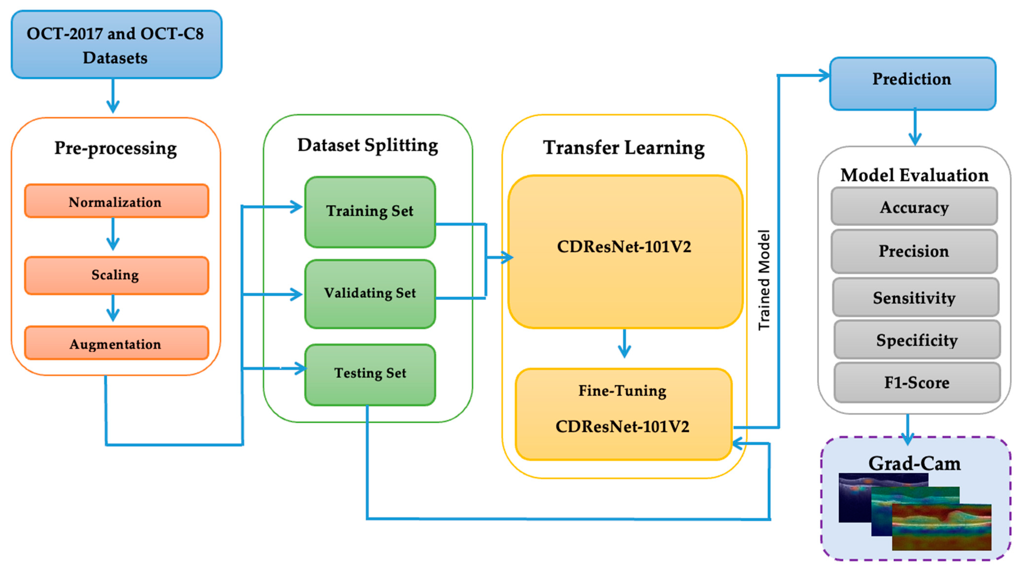
In this section, we describe the evaluation metrics utilized to assess the proposed model. We will cover the overall classification performance, conduct statistical analysis, present ablation studies and visual explanations via Grad-CAM, and compare our findings with previous work.

4.1. Evaluated Performance Metrics

The effectiveness of the six DL models, including CDResNet, EfficientNet-B3, DenseNet201, InceptionV3, MobileNet-V2, and VGG16, is evaluated using Equations (1)–(7).

$$\mathrm{A}\mathrm{c}\mathrm{c}\mathrm{u}\mathrm{r}\mathrm{a}\mathrm{c}\mathrm{y}={\displaystyle \frac{(TP+TN)}{(TP+FP+TN+FN)}}$$

(1)

$$\mathrm{P}\mathrm{r}\mathrm{e}\mathrm{c}\mathrm{i}\mathrm{s}\mathrm{i}\mathrm{o}\mathrm{n}={\displaystyle \frac{TP}{(TP+FP)}}$$

(2)

$$\mathrm{S}\mathrm{e}\mathrm{n}\mathrm{s}\mathrm{i}\mathrm{t}\mathrm{i}\mathrm{v}\mathrm{i}\mathrm{t}\mathrm{y}={\displaystyle \frac{TP}{(TP+FN)}}$$

(3)

$$\mathrm{S}\mathrm{p}\mathrm{e}\mathrm{c}\mathrm{i}\mathrm{f}\mathrm{i}\mathrm{c}\mathrm{i}\mathrm{t}\mathrm{y}={\displaystyle \frac{TN}{(TN+FP)}}$$

(4)

$$\mathrm{F}1-\mathrm{s}\mathrm{c}\mathrm{o}\mathrm{r}\mathrm{e}={\displaystyle \frac{2\times Precision\times Recall}{Precision+Recall}}$$

(5)

$$\mathrm{F}\mathrm{a}\mathrm{l}\mathrm{s}\mathrm{e} \mathrm{N}\mathrm{e}\mathrm{g}\mathrm{a}\mathrm{t}\mathrm{i}\mathrm{v}\mathrm{e} \mathrm{R}\mathrm{a}\mathrm{t}\mathrm{e} (\mathrm{F}\mathrm{N}\mathrm{R})={\displaystyle \frac{FN}{TP+FN}}$$

(6)

$$\mathrm{N}\mathrm{e}\mathrm{g}\mathrm{a}\mathrm{t}\mathrm{i}\mathrm{v}\mathrm{e} \mathrm{P}\mathrm{r}\mathrm{e}\mathrm{d}\mathrm{i}\mathrm{c}\mathrm{t}\mathrm{i}\mathrm{v}\mathrm{e} \mathrm{V}\mathrm{a}\mathrm{l}\mathrm{u}\mathrm{e} (\mathrm{N}\mathrm{P}\mathrm{V})={\displaystyle \frac{TN}{TN+FN}}$$

(7)

True positive (TP): This term refers to the number of instances accurately recognized as belonging to the positive class. True negative (TN): This indicates the number of instances correctly identified as belonging to the negative class. False positive (FP): This represents the number of instances incorrectly identified as belonging to the positive class. False negative (FN): This signifies the number of instances incorrectly identified as belonging to the negative class.

Accuracy refers to the ratio of instances that are correctly classified compared to the total number of instances. Precision, also known as the positive predictive value (PPV), evaluates the proportion of true positive predictions against the total number of positive predictions made. Sensitivity (recall), often referred to as the true positive rate (TPR), measures the proportion of actual positive cases that are correctly identified. Specificity indicates the percentage of true negative results in relation to all actual negative cases. In simpler terms, it assesses how effectively a test identifies individuals who do not have the condition being tested for. F1-score: This metric combines precision and recall by calculating their harmonic mean, providing a single value that balances both metrics effectively. FNR is the percentage of actual positive cases that are incorrectly labeled as negative outcomes. NPV measures the percentage of accurate negative predictions relative to the total number of negative predictions made.

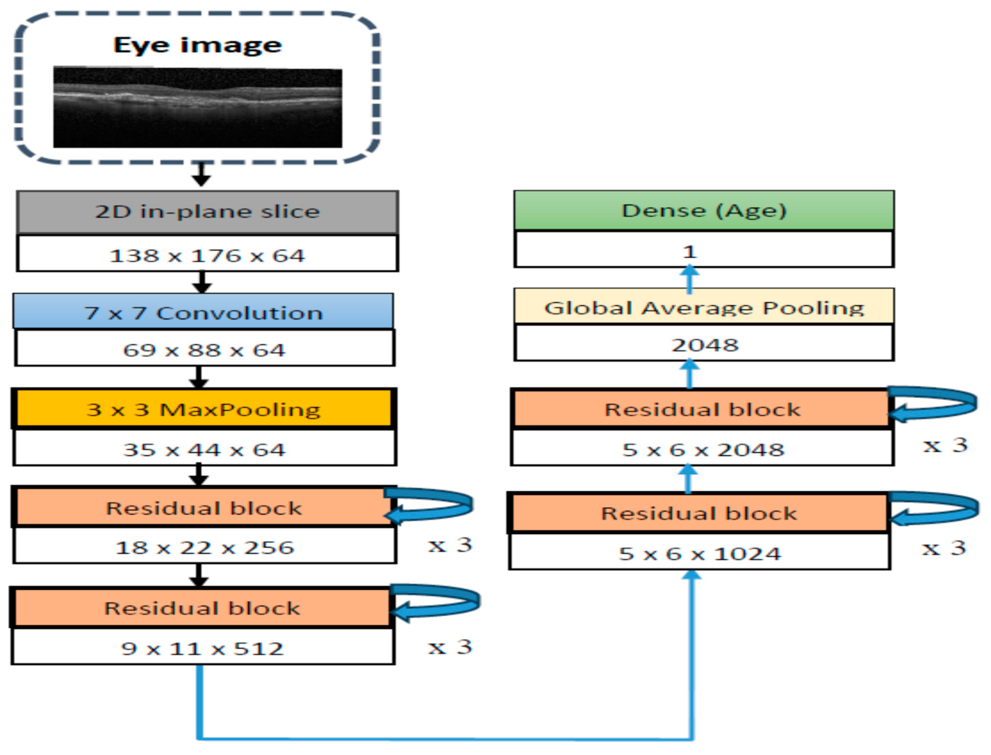
4.2. The CDResNet101-V2 Model Evaluation

In this study, we conducted two experiments using the OCT-2017 and OCT-C8 datasets for multiclass classification in the Kaggle environment. The experiments were performed on a system equipped with an Intel Core i9-13900K CPU operating at 64 GB DDR5 RAM. We utilized Python version 3 and the TensorFlow library, which is a well-known DL framework developed by Google. TensorFlow is commonly used for building and deploying DL and ML models, particularly in the fields of DL and AI.

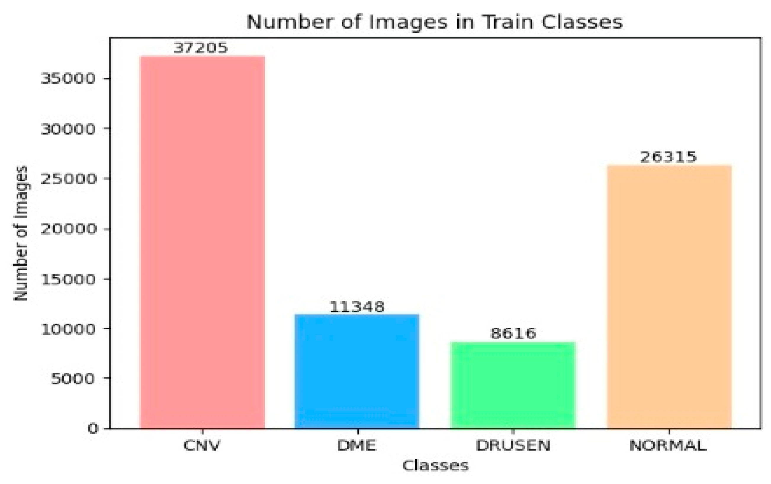
The OCT-2017 dataset was split into three sections: The training set had 83,484 images, the test set included 968 images, and the validation set contained 32 images. The OCT-C8 dataset was also divided into three parts: The training set consisted of 18,400 images, with both the test and validation sets each containing 2800 images. We conducted two experiments focusing on transfer learning to pre-train six DL models. In the initial transfer learning phase, we performed supervised pre-training using the ImageNet dataset to train these six DL models. Subsequently, we carried out the fine-tuning phase using the training sets from the two OCT datasets. At the end of the experiment, we employed evaluation metrics (as specified in Equations (1)–(7)) to evaluate the performance of the six DL models.

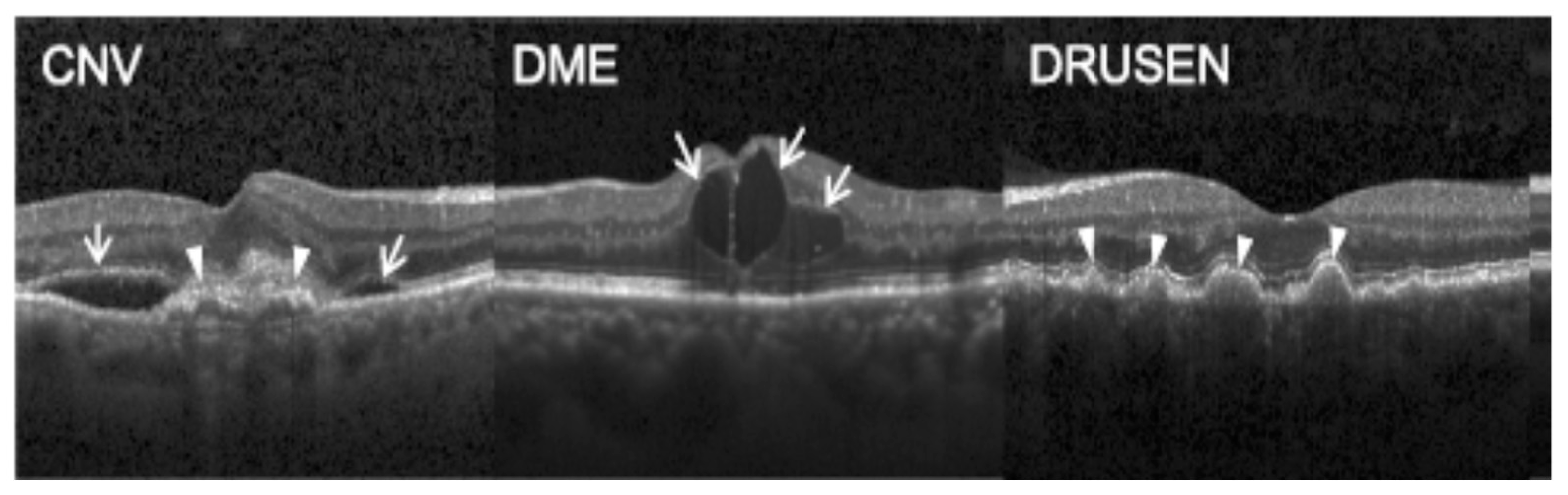
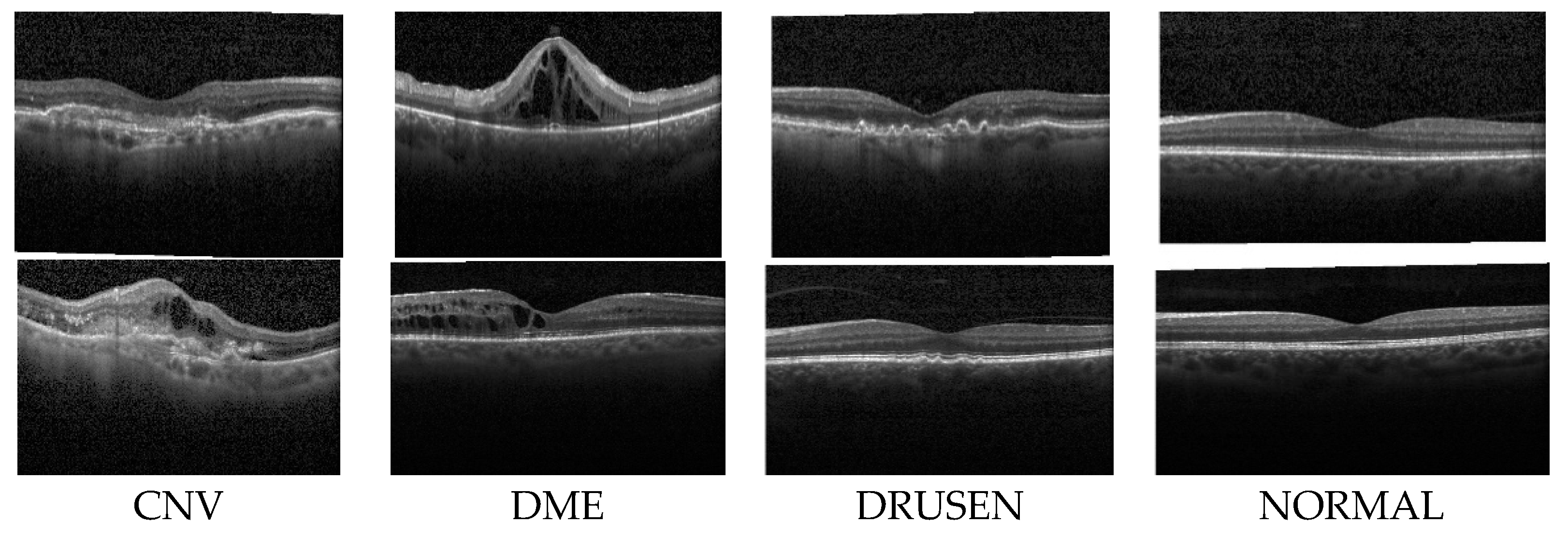
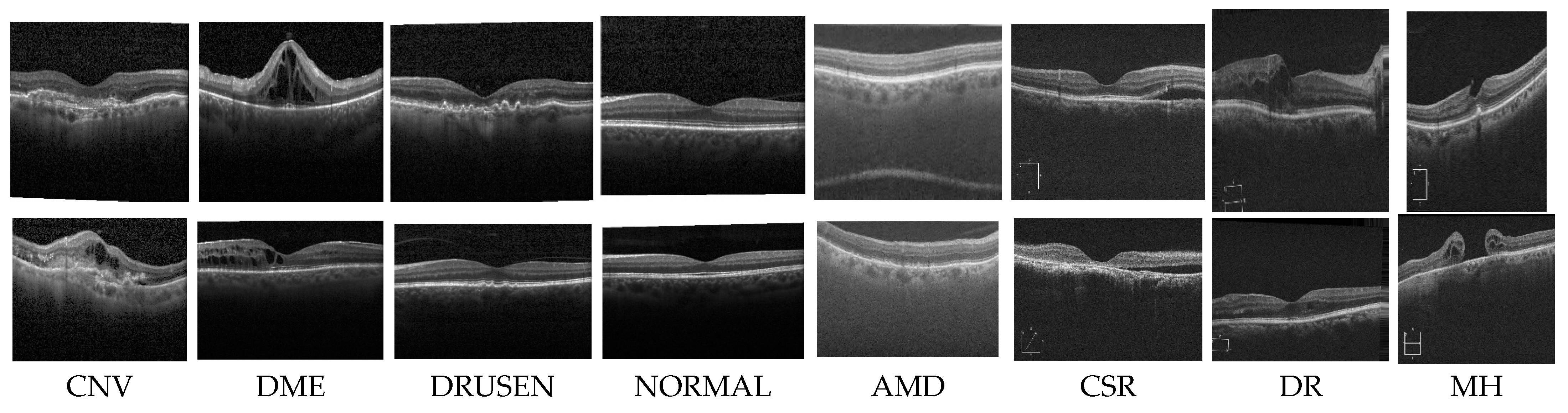
In the first experiment, we conducted a multiclass classification of EDs using the OCT-2017 dataset. This dataset consists of four classes: normal, CNV, DME, and drusen.

Table 5. The results of the six DL models on the test set of the OCT-2017 dataset.

DL Model	Accuracy (%)	Specificity (%)	FNR (%)	NPV (%)	Precision (%)	Recall (%)	F1-Score (%)
CDResNet101-V2	99.90	99.93	0.21	99.93	99.80	99.79	99.79
MobileNet-V2	99.69	99.79	0.62	99.80	99.40	99.38	99.38
EfficinetNet-B0	99.59	99.72	0.83	99.73	99.20	99.17	99.18
EfficinetNet-B3	96.85	97.90	6.30	97.99	94.89	93.70	93.79
NASNetMobile	99.48	99.66	1.03	99.66	99.01	98.97	98.97
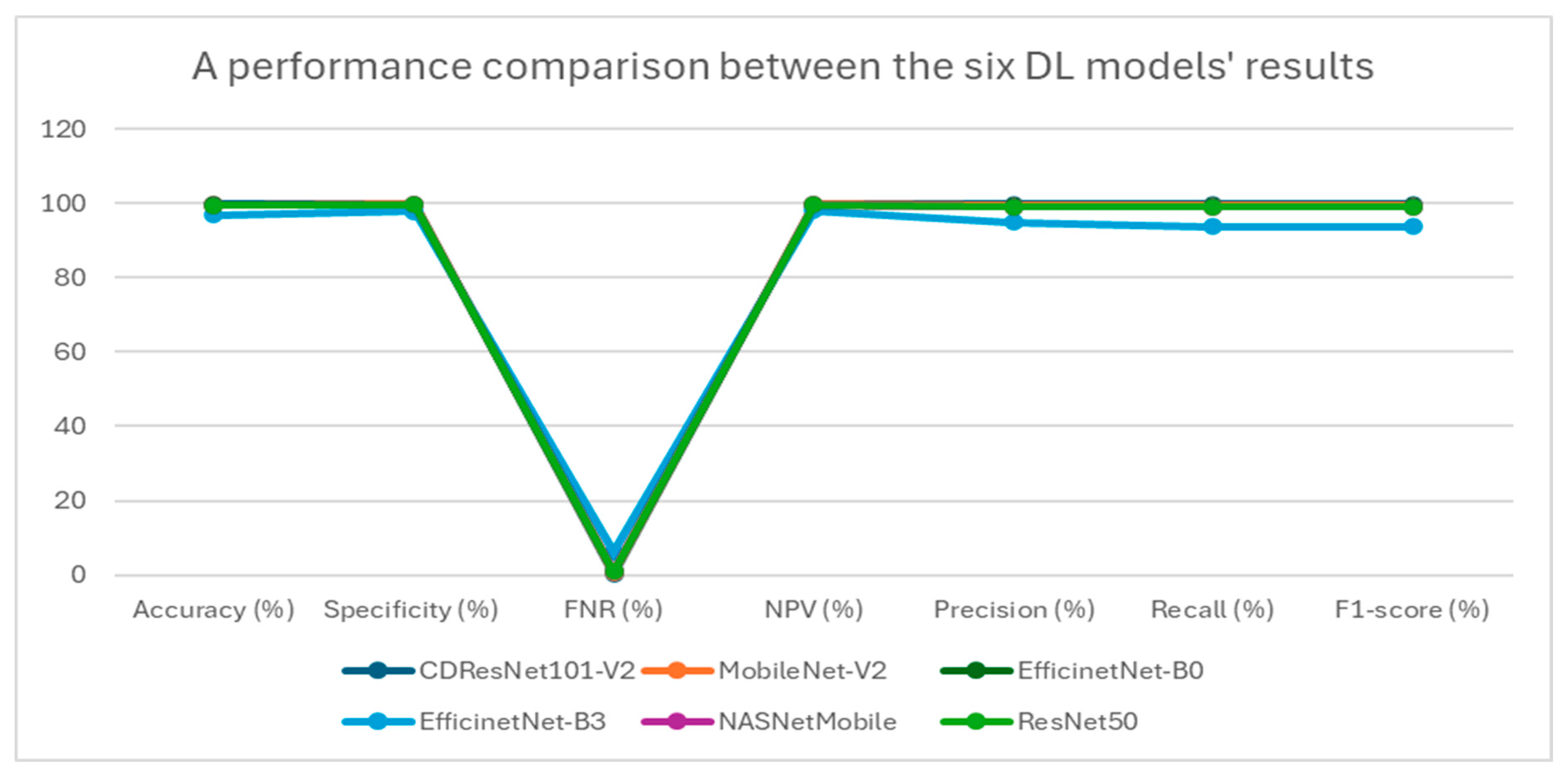
ResNet50	99.54	99.69	0.93	99.69	99.10	99.07	99.07

presents a summary of the performance metrics for the following models: CDResNet101-V2, MobileNet-V2, EfficinetNet-B0, EfficinetNet-B3, NASNetMobile, and ResNet50. The metrics include accuracy, specificity, FNR, NPV, precision, recall, and F1-score. Table 5 and Figure 11 display the performance metrics for the six DL models. The CDResNet101-V2 model achieved the highest accuracy rate of 99.90%, with a specificity of 99.93% and an F1-score of 99.79%. Importantly, it also recorded the lowest FNR at 0.21%, highlighting its exceptional detection capability. Furthermore, the precision of 99.80% and recall of 99.79% illustrate its balanced performance in identifying true positives.

MobileNet-V2 achieved an accuracy of 99.69%, which is marginally lower than that of CDResNet101-V2. The FNR was recorded at 0.62%, with a specificity of 99.79% and a NPV of 99.80%. The F1-score was noted at 99.38%, indicating strong performance, although it was slightly less effective compared to CDResNet101-V2.

EfficientNet-B0 achieved an accuracy of 99.59% and demonstrated a specificity of 99.72% along with an F1-score of 99.18%. The FNR was recorded at 0.83%, indicating a slightly higher error rate than the leading models.

EfficientNet-B3 had the lowest accuracy at 96.85%, with the highest FNR of 6.30%, highlighting a significant performance gap. Its F1-score was 93.79%, and specificity was 97.90%, which was the lowest among the models compared.

NASNetMobile achieved an accuracy of 99.48%, with a specificity of 99.66% and an F1-score of 98.97%. The FNR was noted at 1.03%, suggesting a relatively higher level of misclassification compared to MobileNet-V2 and CDResNet101-V2.

ResNet50 achieved an accuracy of 99.54% and a specificity of 99.69%, with an FNR of 0.93%. Its F1-score was 99.07%, indicating a strong performance, though slightly lower than that of MobileNet-V2.

In summary, CDResNet101-V2 consistently outperformed the other models across nearly all metrics, showcasing greater effectiveness and reliability. In contrast, EfficientNet-B3 exhibited significant performance limitations.

Table 6. The results of the six DL models for the four classes.

	Class	Accuracy (%)	Specificity (%)	FNR (%)	NPV (%)	Precision (%)	Recall (%)	F1-Score (%)
CDResNet101-V2	CNV	99.79	99.72	0.00	100.00	99.18	100.00	99.59
	DME	99.90	100.00	0.41	99.86	100.00	99.59	99.79
	Drusen	99.90	100.00	0.41	99.86	100.00	99.59	99.79
	Normal	100.00	100.00	0.00	100.00	100.00	100.00	100.00
	Average	99.90	99.93	0.21	99.93	99.80	99.79	99.79
MobileNet-V2	CNV	99.38	99.17	0.00	100.00	97.58	100.00	98.78
	DME	100.00	100.00	0.00	100.00	100.00	100.00	100.00
	Drusen	99.38	100.00	2.48	99.18	100.00	97.52	98.74
	Normal	100.00	100.00	0.00	100.00	100.00	100.00	100.00
	Average	99.69	99.79	0.62	99.80	99.40	99.38	99.38
EfficinetNet-B0	CNV	99.17	98.90	0.00	100.00	96.80	100.00	98.37
	DME	99.79	100.00	0.83	99.73	100.00	99.17	99.59
	Drusen	99.38	100.00	2.48	99.18	100.00	97.52	98.74
	Normal	100.00	100.00	0.00	100.00	100.00	100.00	100.00
	Average	99.59	99.72	0.83	99.73	99.20	99.17	99.18
EfficinetNet-B3	CNV	93.90	91.87	0.00	100.00	80.40	100.00	89.13
	DME	97.93	100.00	8.26	97.32	100.00	91.74	95.69
	Drusen	95.76	100.00	16.94	94.65	100.00	83.06	90.74
	Normal	99.79	99.72	0.00	100.00	99.18	100.00	99.59
	Average	96.85	97.90	6.30	97.99	94.89	93.70	93.79
NASNetMobile	CNV	98.97	98.62	0.00	100.00	96.03	100.00	97.98
	DME	99.90	100.00	0.41	99.86	100.00	99.59	99.79
	Drusen	99.07	100.00	3.72	98.78	100.00	96.28	98.11
	Normal	100.00	100.00	0.00	100.00	100.00	100.00	100.00
	Average	99.48	99.66	1.03	99.66	99.01	98.97	98.97
ResNet50	CNV	99.17	98.90	0.00	100.00	96.80	100.00	98.37
	DME	99.48	100.00	2.07	99.32	100.00	97.93	98.96
	Drusen	99.59	99.86	1.24	99.59	99.58	98.76	99.17
	Normal	99.90	100.00	0.41	99.86	100.00	99.59	99.79
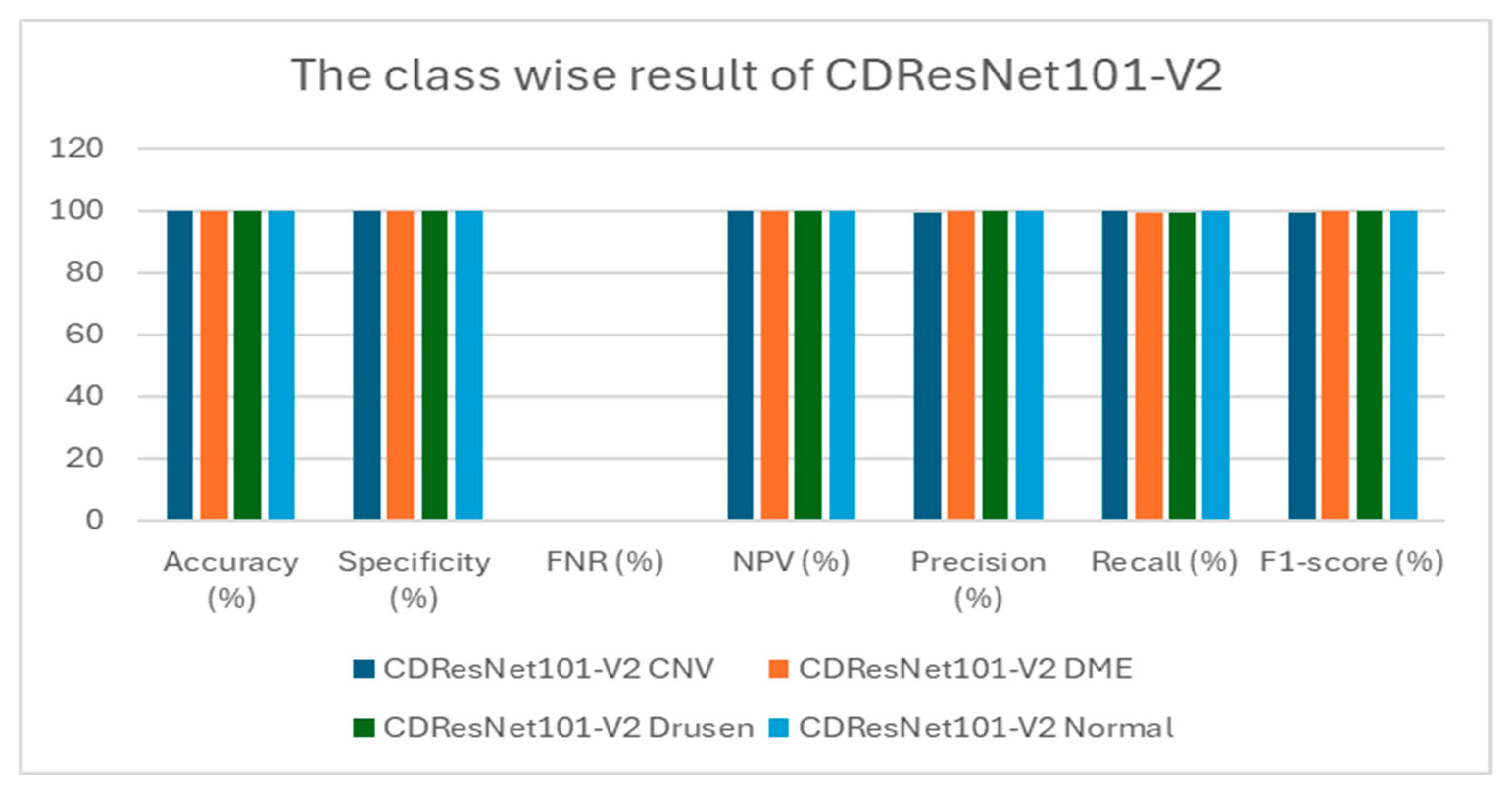
	Average	99.54	99.69	0.93	99.69	99.10	99.07	99.07

presents class-wise evaluation metrics for the six DL models on the test set of the OCT-2017 dataset that contains four classes: CNV, DME, drusen, and normal. In Table 6 and Figure 12, for the CNV class, CDResNet101-V2 achieved an accuracy of 99.79% and a specificity of 99.72%. Notably, it recorded an FNR of 0.00%, indicating that there were no missed true positive cases. The precision was 99.18%, and recall was perfect at 100%, resulting in an F1-score of 99.59%. This indicates that the model was highly reliable in detecting CNV without missing any true positive cases. For the DME class, it demonstrated an impressive accuracy of 99.90% and a specificity of 100%. The FNR was minimal at 0.41%. With precision at 100% and recall reaching 99.59%, the F1-score was calculated at 99.79%. The model exhibited an excellent balance between sensitivity and specificity for DME detection. For the drusen class, CDResNet101-V2 was similar to DME; it achieved an accuracy of 99.90%, with a specificity of 100% and an FNR of 0.41%. Both precision and recall were 100% and 99.59%, respectively, yielding an F1-score of 99.79%. The results demonstrated that the model was equally effective in detecting drusen with minimal false negatives. For the normal class, CDResNet101-V2 performed flawlessly for normal images, achieving 100% in accuracy, specificity, NPV, precision, recall, and F1-score, with an FNR of 0.00%. This suggests perfect classification of normal retinal images, with no false positives or negatives.

MobileNet-V2 reached an accuracy of 99.38%, with an F1-score of 98.78% and 100% recall for the CNV class. It performed excellently in the DME class, achieving perfect scores across all categories (100%). However, for the drusen class, it recorded an accuracy of 99.38%, with a higher FNR of 2.48% and an F1-score of 98.74%, indicating a slight decrease in performance. The normal class also displayed perfect metrics (100%).

EfficientNet-B0 achieved an accuracy of 99.17% for the CNV class, with an F1-score of 98.37% and 100% recall. In the DME class, it scored 99.79% accuracy, boasting 100% specificity and an F1-score of 99.59%. For the drusen class, it attained an accuracy of 99.38%, accompanied by a higher FNR of 2.48% and an F1-score of 98.74%. The normal class demonstrated perfect metrics (100%).

EfficientNet-B3 showed a lower accuracy of 93.90% for the CNV class, with relatively low precision at 80.40% and an F1-score of 89.13%. In the DME class, it achieved 97.93% accuracy, with a higher FNR of 8.26% and an F1-score of 95.69%. For the drusen class, its accuracy was 95.76%, with a significantly high FNR of 16.94% and an F1-score of 90.74%. The normal class exhibited near-perfect performance, with an F1-score of 99.59%.

NASNetMobile recorded an accuracy of 98.97%, with 100% recall and an F1-score of 97.98% for the CNV class. It performed excellently in the DME class, with perfect metrics across all categories (100%). For the drusen class, it achieved an accuracy of 99.07%, with an FNR of 3.72% and an F1-score of 98.11%. It also demonstrated perfect performance in the normal class (100%).

ResNet50 attained an accuracy of 99.17%, with an F1-score of 98.37% and 100% recall for the CNV class. In the DME class, it scored 99.48% accuracy, with an F1-score of 98.96% and an FNR of 2.07%. For the drusen class, its accuracy was 99.59%, yielding an F1-score of 99.17%. In the normal class, it achieved nearly perfect results, with an F1-score of 99.79%.

In conclusion, CDResNet101-V2 exhibited the best overall performance, achieving the highest metrics across all classes. Conversely, EfficientNet-B3 faced the most challenges, particularly in the drusen and DME classes, highlighting its limitations. Other models like MobileNet-V2 and NASNetMobile demonstrated consistent and reliable performance, although they did not reach the exceptional results of CDResNet101-V2.

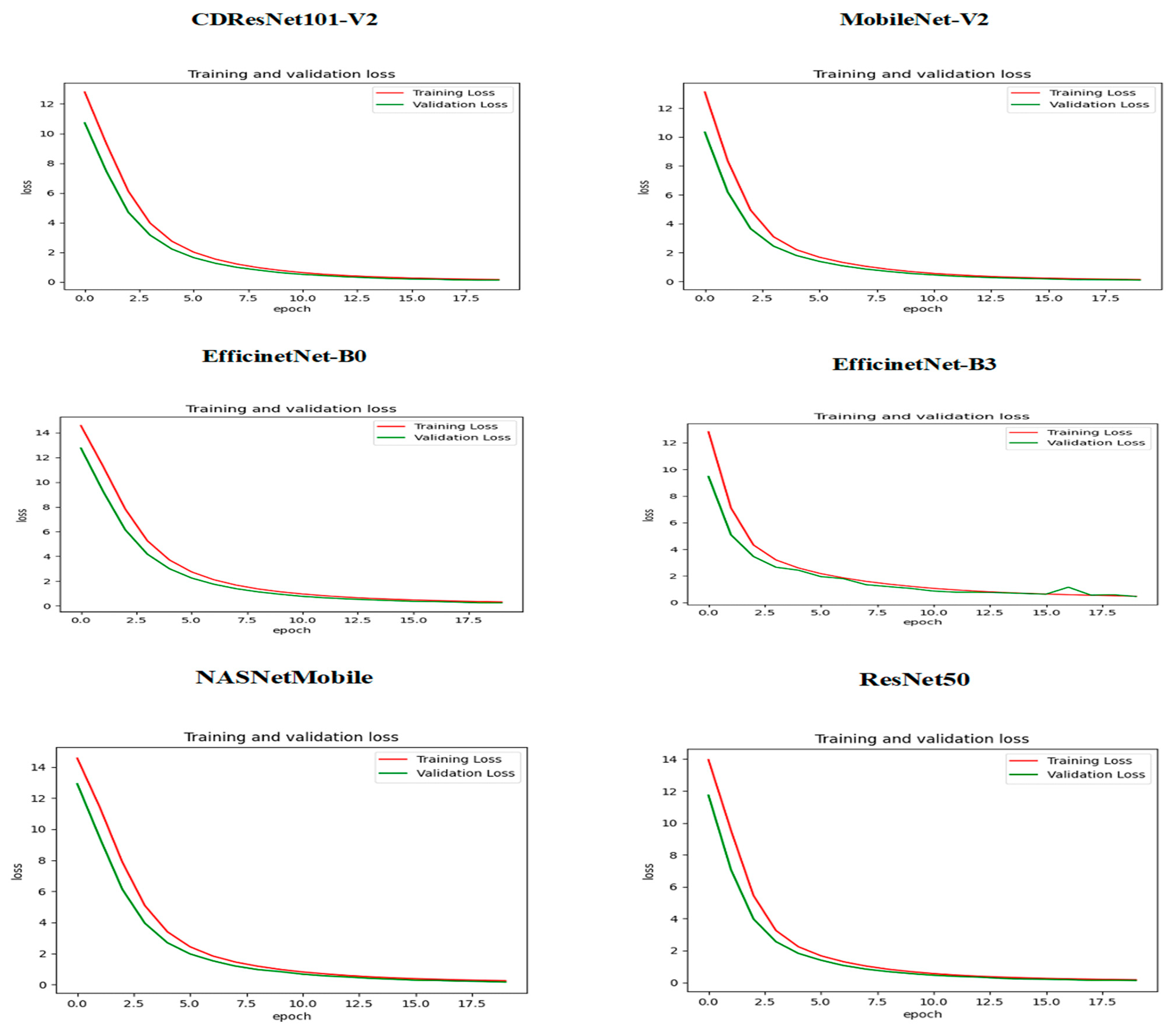
Figure 13 illustrates how the training and validation loss changed over epochs while training six DL models. At the beginning, specifically at epoch 0, the training loss was significantly high, indicating that the models were not initially well-fitted to the data. The validation loss was also high but slightly lower than the training loss. As the training progressed, a steady decline in both losses was observed, suggesting that the models were improving their learning and reducing errors over time. By approximately epoch 15, both the training and validation losses approached zero, signaling that the models had achieved a robust fit to the data. The closeness of the training and validation curves indicated a low risk of overfitting, as they displayed similar trends throughout the training period. The small gap between the training loss (shown by the red curve) and validation loss (represented by the green curve) in the later epochs highlighted the models’ capacity to generalize effectively to new, unseen data. In conclusion, Figure 13 demonstrates that the training of the six DL models successfully reduced both training and validation losses, reaching convergence with minimal signs of overfitting. Figure 14 shows the relationship between training and validation accuracy and the number of epochs during the training of six DL models. At the beginning of the training (epoch 0) for the CDResNet101-V2, MobileNet-V2, EfficinetNet-B0, NASNetMobile, and ResNet50 models, the training accuracy (shown by the red curve) was low, indicating that the model’s initial performance was not very good. In contrast, the validation accuracy (shown by the green curve) started at a higher level than the training accuracy, suggesting better initial performance on the validation dataset. As the epochs progressed, the training accuracy steadily increased. The validation accuracy experienced some fluctuations but remained relatively high throughout the training process. By around epoch 15, the training accuracy approached 100%, indicating that the model fit the training data very well. The validation accuracy also stayed close to 100% over the epochs, with only slight variations, demonstrating that the model had strong generalization capabilities on the validation dataset.

The training and validation accuracy curves in Figure 14 showed minimal divergence, indicating that the model effectively avoided overfitting and maintained a good balance between training and validation performance. Overall, the plot illustrated that the model successfully improved its training accuracy while keeping consistently high validation accuracy, showcasing its strong learning and generalization abilities.

In the initial epoch (epoch 0) of the EfficientNet-B3 model, training accuracy was relatively low, suggesting that the model struggled to perform well on the training dataset at the beginning. Conversely, validation accuracy started at a higher level than training accuracy but displayed significant variations in the early epochs. As training progressed, there was a consistent increase in training accuracy, indicating effective learning and improvement. However, validation accuracy showed notable fluctuations, with occasional spikes and declines, reflecting variability in the model’s generalization ability. In the middle to later epochs, validation accuracy experienced sharp declines at certain points, diverging from the steadily increasing training accuracy. This divergence hinted at potential overfitting or sensitivity to the validation dataset. By the end of the training, training accuracy approached 90%, signifying strong performance on the training data. Meanwhile, validation accuracy stabilized around 90% but continued to exhibit variability, highlighting inconsistencies in generalization. In conclusion, despite the model’s progress on the training dataset, the fluctuations observed in validation accuracy suggested possible overfitting or sensitivity to the characteristics of the validation dataset.

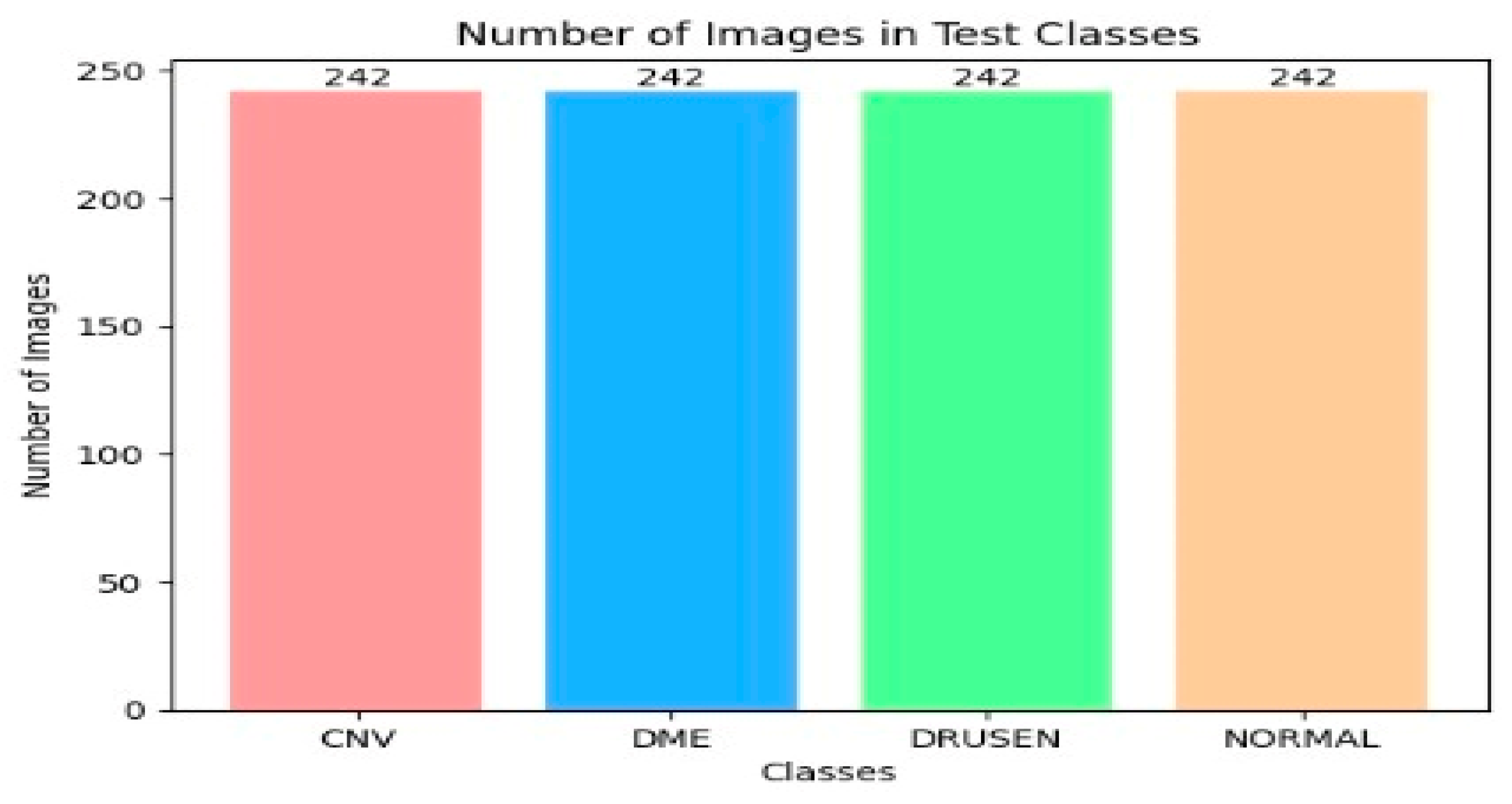
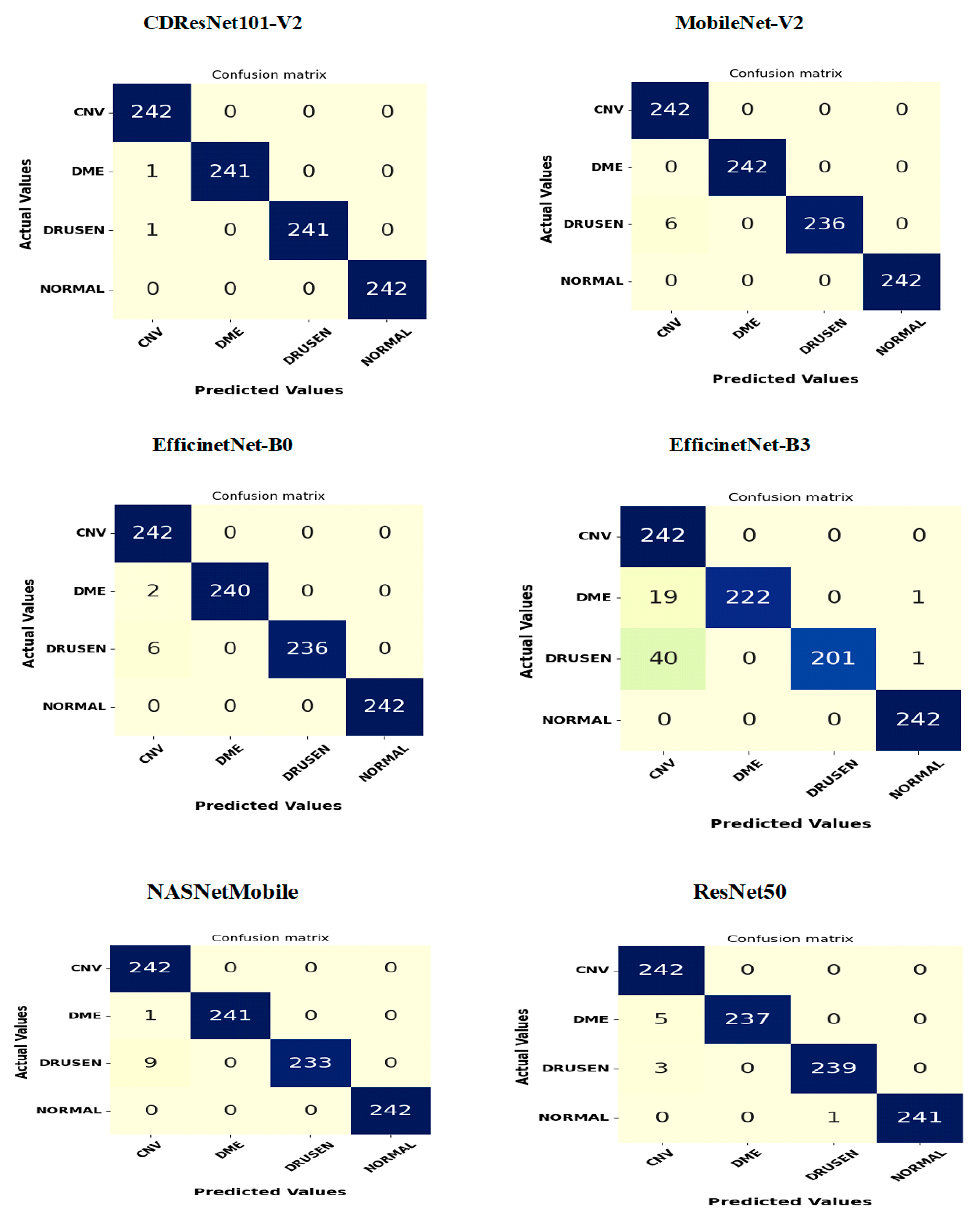
Figure 15 shows the confusion matrices for six DL models tested on the OCT-2107 dataset, consisting of 242 samples categorized into four groups: CNV, DME, drusen, and normal. The CDResNet101-V2 model demonstrated exceptional performance in both the CNV and normal categories, achieving an impressive accuracy of 100%. It accurately classified almost all instances, with only two misclassifications: one CNV instance was incorrectly identified, and one drusen instance was misclassified as CNV. Overall, the CDResNet101-V2 model effectively categorized all four classes of EDs.

The MobileNet-V2 model also achieved a high accuracy of 100% for the CNV, DME, and normal categories, successfully classifying all instances. However, it misclassified six drusen instances as CNV, resulting in an overall accuracy of 97.5% for that category.

The EfficientNet-B0 model accurately identified all 242 actual instances of CNV and normal, both achieving perfect accuracy of 100%. It correctly classified 240 out of 242 DME instances, resulting in an accuracy of 99.17%, with two DME instances misclassified as CNV. Additionally, it accurately classified 236 drusen instances, but six were incorrectly predicted as CNV, leading to a 97.5% accuracy for that class. The model performed exceptionally well with CNV and normal while showing only minor misclassifications in DME and drusen.

The EfficientNet-B3 model also achieved perfect predictions for all 242 actual CNV and normal instances. Among the DME instances, it correctly classified 222, while 19 were misclassified as CNV and one as normal. For drusen, 201 instances were correctly classified, but 40 were misidentified as CNV and one as normal. This model excelled in classifying CNV and normal but showed some confusion between DME and CNV, as well as drusen and CNV, with a few isolated misclassifications of DME and drusen as normal.

The NASNetMobile model performed excellently, accurately classifying all 242 actual CNV and normal instances. It correctly identified 241 DME instances, but one was misclassified as CNV. For drusen, 233 instances were accurately classified, but nine were misidentified as CNV. Overall, this model achieved perfect classification for CNV and normal, with slight misclassifications in DME and drusen.

Lastly, the ResNet50 model accurately classified all 242 actual CNV instances. It correctly predicted 237 DME instances while misclassifying five as CNV. For drusen, 239 instances were correctly classified, while three were incorrectly labeled as CNV. The model also correctly identified 241 normal instances, with one misclassified as drusen. In summary, ResNet50 demonstrated high accuracy across CNV, DME, and normal categories, with only a few misclassifications, mostly affecting DME and drusen.

In the second experiment, we conducted a multiclass classification of EDs using the OCT-C8 dataset. This dataset consists of eight classes: AMD, CNV, CSR, DME, DR, drusen, MH, and normal.

Table 7. The results of the six DL models on the test set of the OCT-C8 dataset.

DL Model	Accuracy (%)	Specificity (%)	FNR (%)	NPV (%)	Precision (%)	Recall (%)	F1-Score (%)
CDResNet101-V2	99.28	99.59	2.89	99.59	97.14	97.11	85.55
MobileNet-V2	98.91	87.00	4.36	87.00	83.33	83.27	83.27
EfficinetNet-B0	99.04	99.45	3.86	99.45	96.22	96.14	96.14
EfficinetNet-B3	99.18	87.31	2.90	87.21	85.39	84.73	85.05
NASNetMobile	98.13	98.93	7.46	98.94	93.01	92.54	92.54
ResNet50	99.21	99.55	3.14	99.55	96.93	96.86	96.85

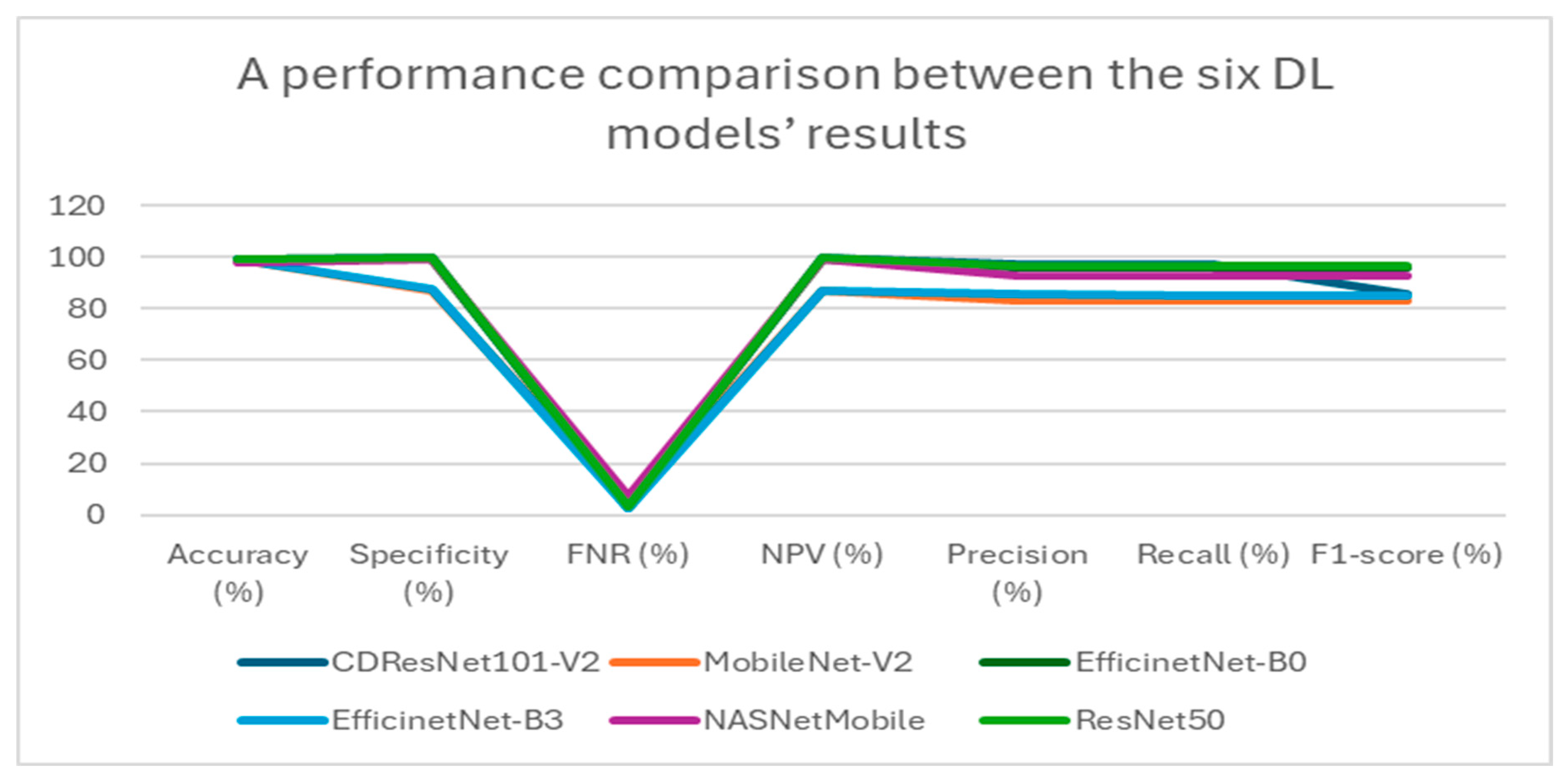
and Figure 16 present a summary of the performance metrics for the following models: CDResNet101-V2, MobileNet-V2, EfficinetNet-B0, EfficinetNet-B3, NASNetMobile, and ResNet50. The metrics include accuracy, specificity, FNR, NPV, precision, recall, and F1-score. Table 7 displays the performance metrics for six DL models. CDResNet101-V2 model achieved remarkable results, with an accuracy of 99.28% and a specificity of 99.59%. It had a low FNR of 2.89%, demonstrating strong classification ability across various categories. Its precision was 97.14%, and recall stood at 97.11%, resulting in an impressive F1-score of 85.55%.

MobileNet-V2, achieving an accuracy of 98.91%, had a significantly lower specificity of 87.00% compared to others. It recorded an FNR of 4.36% and an NPV of 87.00%, indicating areas for improvement. The precision was 83.33%, with a recall of 83.27%, leading to a lower F1-score of 83.27%. Inconsistent management of class imbalances was noted.

EfficientNet-B0 achieved a strong overall performance, with an accuracy of 99.04% and a specificity of 99.45%. It maintained a low FNR of 3.86% and a high NPV of 99.45, reflecting reliability in negative predictions. The precision recorded was 96.22%, with a recall at 96.14%, culminating in an F1-score of 96.14%. It demonstrated stable and dependable performance across various categories.

EfficientNet-B3 had an accuracy of 99.18%. Its specificity was slightly lower at 87.31% compared to EfficientNet-B0. It maintained a low FNR of 2.90%, while the NPV at 87.21% was comparable to its specificity. The precision was 85.39%, and recall was 84.73%, resulting in a slightly lower F1-score of 85.05%.

NASNetMobile achieved an accuracy of 98.13% and a specificity of 98.93%, which were respectable but slightly lower than some other models. However, it recorded the highest FNR at 7.46%, impacting on its overall reliability. The precision was strong at 93.01%, and the recall was 92.54%, resulting in an F1-score of 92.54%. While performing well, it faced challenges due to a higher rate of false negatives.

ResNet50 achieved excellent results, with an accuracy of 99.21% and a specificity of 99.55%. It maintained a low FNR of 3.14% and a high NPV of 99.55%, ensuring robust classification. With precision at 96.93% and recall at 96.86%, it produced an F1-score of 96.85%. This model exhibited consistent and reliable performance across all metrics.

In conclusion, CDResNet101-V2 and ResNet50 demonstrated the most reliable and high-performing metrics overall. EfficientNet-B0 closely followed, with slightly lower performance in certain areas. MobileNet-V2 and EfficientNet-B3 showed variability, especially in specificity and precision under certain conditions. NASNetMobile, while delivering competitive outcomes, was impacted by a higher FNR, affecting its overall reliability.

Table 8. The results of the six DL models for the eight classes.

	Class	Accuracy (%)	Specificity (%)	FNR (%)	NPV (%)	Precision (%)	Recall (%)	F1-Score (%)
CDResNet101-V2	AMD	100.00	100.00	0.00	100.00	100.00	100.00	100.00
	CNV	98.46	99.02	5.43	99.22	93.24	94.57	93.90
	CSR	99.96	99.96	0.00	100.00	99.72	100.00	99.86
	DME	98.68	99.63	8.00	98.87	97.28	92.00	94.57
	DR	100.00	100.00	0.00	100.00	100.00	100.00	100.00
	DRUSEN	98.36	99.14	7.14	98.98	93.93	92.86	93.39
	MH	99.96	100.00	0.29	99.96	100.00	99.71	99.86
	NORMAL	98.79	98.94	2.29	99.67	92.93	97.71	95.26
	Average	99.28	99.59	2.89	99.59	97.14	97.11	97.10
MobileNet-V2	AMD	100.00	100.00	0.00	100.00	100.00	100.00	100.00
	CNV	97.86	99.18	11.43	98.38	93.94	88.57	91.18
	CSR	99.96	100.00	0.29	99.96	100.00	99.71	99.86
	DME	98.32	99.27	8.29	98.82	94.69	91.71	93.18
	DR	99.93	99.92	0.00	100.00	99.43	100.00	99.72
	DRUSEN	97.18	98.12	9.43	98.65	87.33	90.57	88.92
	MH	99.96	100.00	0.29	99.96	100.00	99.71	99.86
	NORMAL	98.07	98.53	5.14	99.26	90.22	94.86	92.48
	Average	98.91	99.38	4.36	99.38	95.70	95.64	95.65
EfficinetNet-B0	AMD	99.96	99.96	0.00	100.00	99.72	100.00	99.86
	CNV	97.93	99.10	10.29	98.54	93.45	89.71	91.55
	CSR	100.00	100.00	0.00	100.00	100.00	100.00	100.00
	DME	98.54	99.63	9.14	98.71	97.25	90.86	93.94
	DR	99.96	100.00	0.29	99.96	100.00	99.71	99.86
	DRUSEN	97.54	98.61	10.00	98.57	90.26	90.00	90.13
	MH	99.96	99.96	0.00	100.00	99.72	100.00	99.86
	NORMAL	98.39	98.33	1.14	99.83	89.41	98.86	93.89
	Average	99.04	99.45	3.86	99.45	96.22	96.14	96.14
EfficinetNet-B3	AMD	100.00	100.00	0.00	100.00	100.00	100.00	100.00
	CNV	98.39	99.43	8.86	98.74	95.80	91.14	93.41
	CSR	99.96	99.96	0.00	100.00	99.72	100.00	99.86
	DME	98.61	99.47	7.43	98.94	96.14	92.57	94.32
	DR	99.96	100.00	0.29	99.96	100.00	99.71	99.86
	DRUSEN	97.96	98.61	6.57	99.06	90.58	93.43	91.98
	MH	100.00	100.00	0.00	100.00	100.00	100.00	100.00
	NORMAL	98.54	98.78	3.14	99.55	91.87	96.86	94.30
	Average	99.18	99.53	3.29	99.53	96.76	96.71	96.72
NASNetMobile	AMD	99.93	100.00	0.57	99.92	100.00	99.43	99.71
	CNV	97.00	99.14	18.00	97.47	93.18	82.00	87.23
	CSR	98.71	100.00	10.29	98.55	100.00	89.71	94.58
	DME	97.57	99.51	16.00	97.75	96.08	84.00	89.63
	DR	98.61	98.82	2.86	99.59	92.14	97.14	94.58
	DRUSEN	96.25	96.82	7.71	98.87	80.55	92.29	86.02
	MH	99.29	99.39	1.43	99.80	95.83	98.57	97.18
	NORMAL	97.71	97.80	2.86	99.58	86.29	97.14	91.40
	Average	98.13	98.93	7.46	98.94	93.01	92.54	92.54
ResNet50	AMD	100.00	100.00	0.00	100.00	100.00	100.00	100.00
	CNV	98.18	98.45	3.71	99.46	89.87	96.29	92.97
	CSR	100.00	100.00	0.00	100.00	100.00	100.00	100.00
	DME	98.79	99.51	6.29	99.11	96.47	93.71	95.07
	DR	99.96	100.00	0.29	99.96	100.00	99.71	99.86
	DRUSEN	98.00	99.51	12.57	98.23	96.23	87.43	91.62
	MH	99.96	99.96	0.00	100.00	99.72	100.00	99.86
	NORMAL	98.82	98.98	2.29	99.67	93.19	97.71	95.40
	Average	99.21	99.55	3.14	99.55	96.93	96.86	96.85

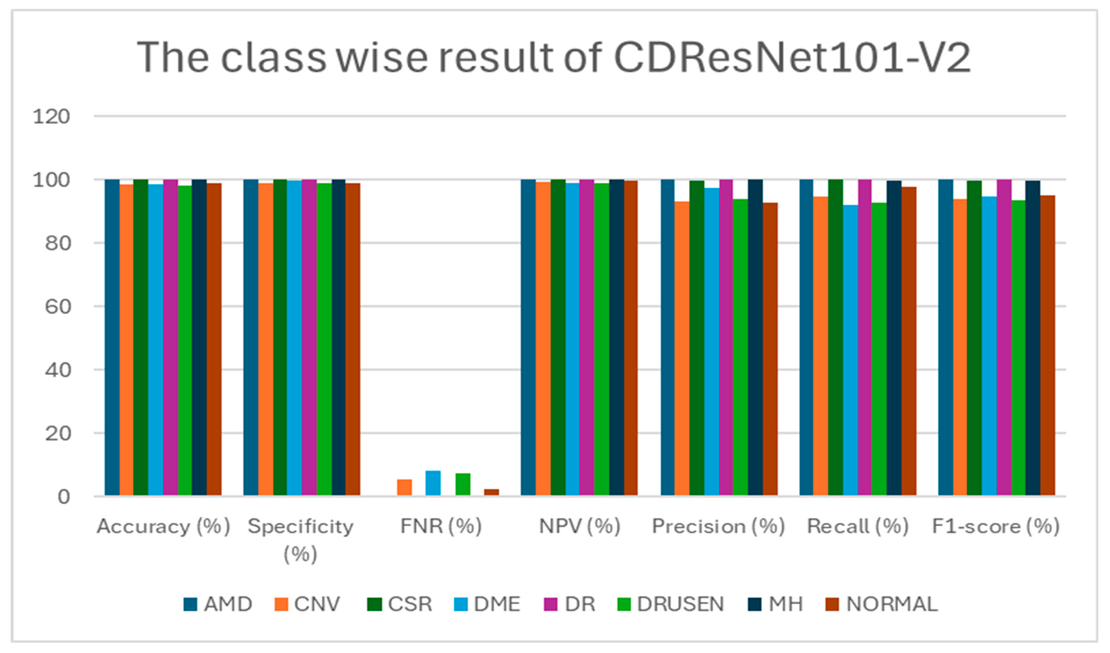
presents class-wise evaluation metrics for six DL models tested on the OCT-C8 dataset, which includes eight classes: AMD, CNV, CSR, DME, DR, drusen, MH, and normal. In Table 8 and Figure 17, The CDResNet101-V2 model showed exceptional performance, achieving 100% accuracy, specificity, and F1-score for the AMD, CSR, DR, and MH classes. However, the CNV, DME, and drusen classes saw a slight decrease in precision and recall, with the highest FNR for DME at 8%. The normal class demonstrated high accuracy at 98.79% and precision at 92.93%, although its recall was slightly lower at 97.71%. On average, the model achieved an impressive accuracy of 99.28% and an F1-score of 97.10%, indicating strong overall effectiveness.

MobileNet-V2 also achieved perfect scores (100%) in the AMD, CSR, and MH categories. However, the CNV and drusen classes had the highest FNRs at 11.43% and 9.43%, respectively, leading to lower F1-scores of 91.18% and 88.92%. While the DME and normal categories maintained high accuracy, they experienced slight reductions in both recall and precision compared to other classes. The average F1-score for this model was slightly lower than that of CDResNet101-V2, at 95.65%.

EfficientNet-B0 maintained consistently high performance across all classes, achieving perfect or near-perfect results for the AMD, CSR, DR, and MH categories. The CNV and drusen classes showed decreased precision (93.45% and 90.26%) and F1-scores (91.55% and 90.13%) due to higher FNRs. The normal category achieved commendable metrics, although its recall was slightly lower at 98.86%. Overall, the performance was competitive but slightly below that of CDResNet101-V2, with an F1-score of 96.14%.

EfficientNet-B3 produced outstanding results, achieving perfect scores for AMD, CSR, and MH. Although the CNV and DME categories saw reduced recall, their precision remained strong, resulting in F1-scores of 93.41% and 94.32%, respectively. The drusen and normal categories showed slight variability but maintained strong overall metrics. The average F1-score for this model was 96.72%, reflecting excellent performance across most classes.

NASNetMobile, while competitive, recorded the lowest overall performance among the tested models. The AMD and MH categories achieved near-perfect metrics, but the CNV and DME classes experienced significant drops in recall and F1-scores (82.00% and 84.00%). The drusen class recorded the lowest precision (80.55%) across all models, negatively impacting its F1-score. On average, this model achieved a respectable F1-score of 92.54%, although lower than the others.

ResNet50 achieved flawless results in the AMD, CSR, DR, and MH classes. The CNV and drusen categories displayed lower precision (89.87% and 96.23%) and higher FNRs compared to the leading models. The DME and normal classes maintained strong metrics, with only minimal declines in precision and recall. The average F1-score for ResNet50 was 96.85%, indicating excellent overall performance, though slightly behind CDResNet101-V2.

In conclusion, CDResNet101-V2 emerged as the top performer, consistently achieving high metrics across all classes. MobileNet-V2 and EfficientNet-B3 closely followed, although with slightly lower metrics in certain categories. In contrast, NASNetMobile exhibited the least favorable performance, with significant variability in F1-scores across the various classes.

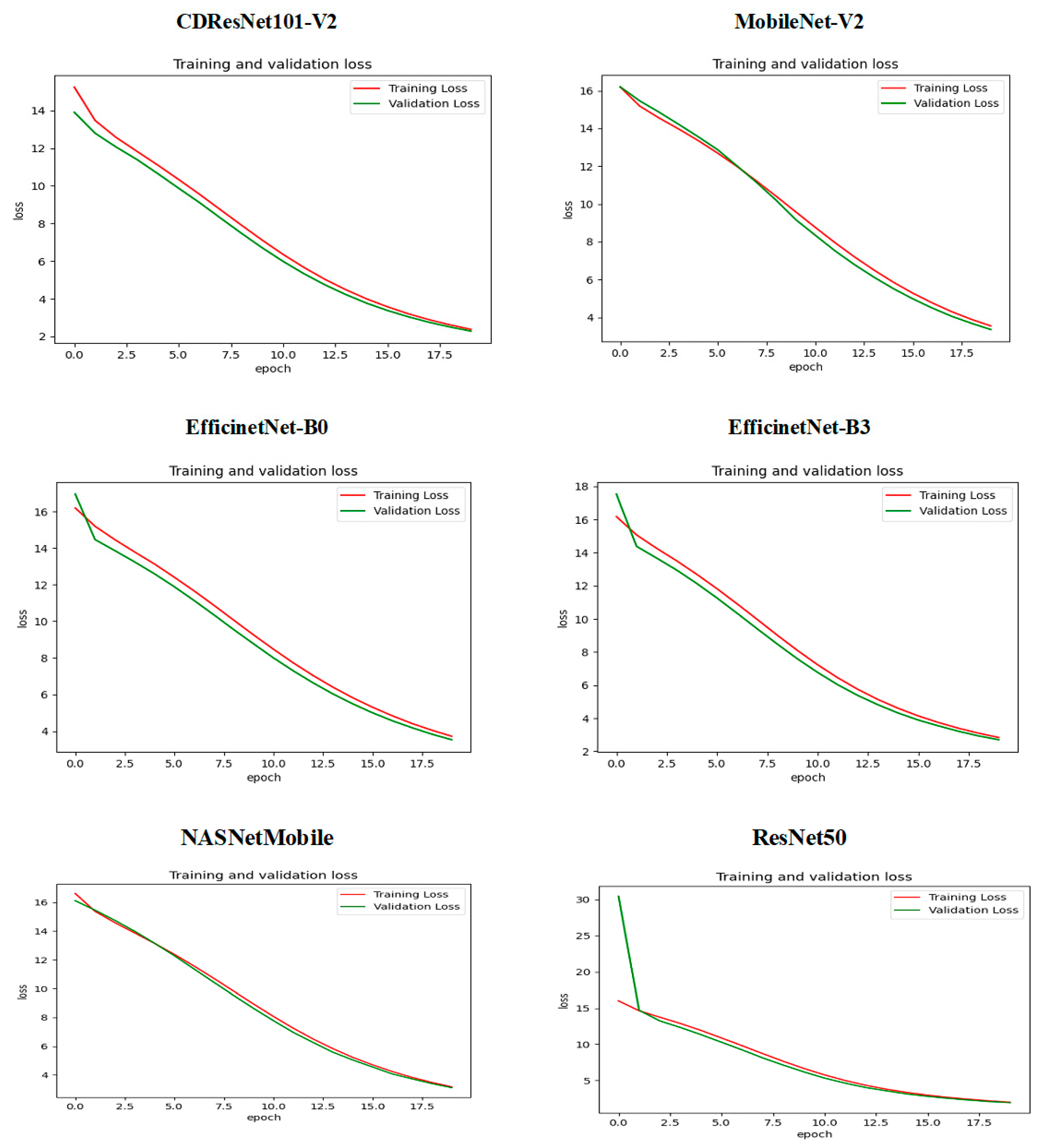
Figure 18 presents the training and validation loss over 18 epochs for the six DL models. The x-axis denotes the number of epochs, while the y-axis represents the loss values. For the CDResNet101-V2 model, the training loss (in red) started at approximately 14 and consistently decreased throughout the training process, nearing 2 by the 18th epoch. The validation loss (in green) followed a similar trend, starting around 14 and steadily declining to stabilize near 2 by the training’s conclusion. The close alignment between the training and validation loss curves indicates that the model effectively reduced loss during training without overfitting. Both curves maintained a continuous downward trend, demonstrating the model’s ability to generalize well to the data.

In the case of MobileNet-V2, EfficientNet-B0, EfficientNet-B3, and NASNetMobile, the training loss began at about 16 and gradually decreased, ultimately reaching around 4 by the 18th epoch. The validation loss mirrored this pattern, also starting near 16 and consistently declining to stabilize around 4 by the final epoch. The strong correlation between the training and validation loss curves suggests that these models effectively minimized loss during training without overfitting, with both curves reflecting a steady downward trajectory indicative of their generalization capabilities across the data.

For the ResNet50 model, the training loss commenced at a notably higher value of about 25 and steadily decreased over the epochs, stabilizing at around 5 by the end of the training. Interestingly, the validation loss began even higher than the training loss, peaking at approximately 30 before sharply declining and closely aligning with the training loss. By the final epochs, the validation loss also stabilized around 5. The consistent reduction in both training and validation loss indicates that the model successfully minimized loss during training. The convergence of the two curves suggests that the model generalized well to unseen data without overfitting. However, the initial spike in validation loss may imply early instability, which was addressed in the subsequent epochs. 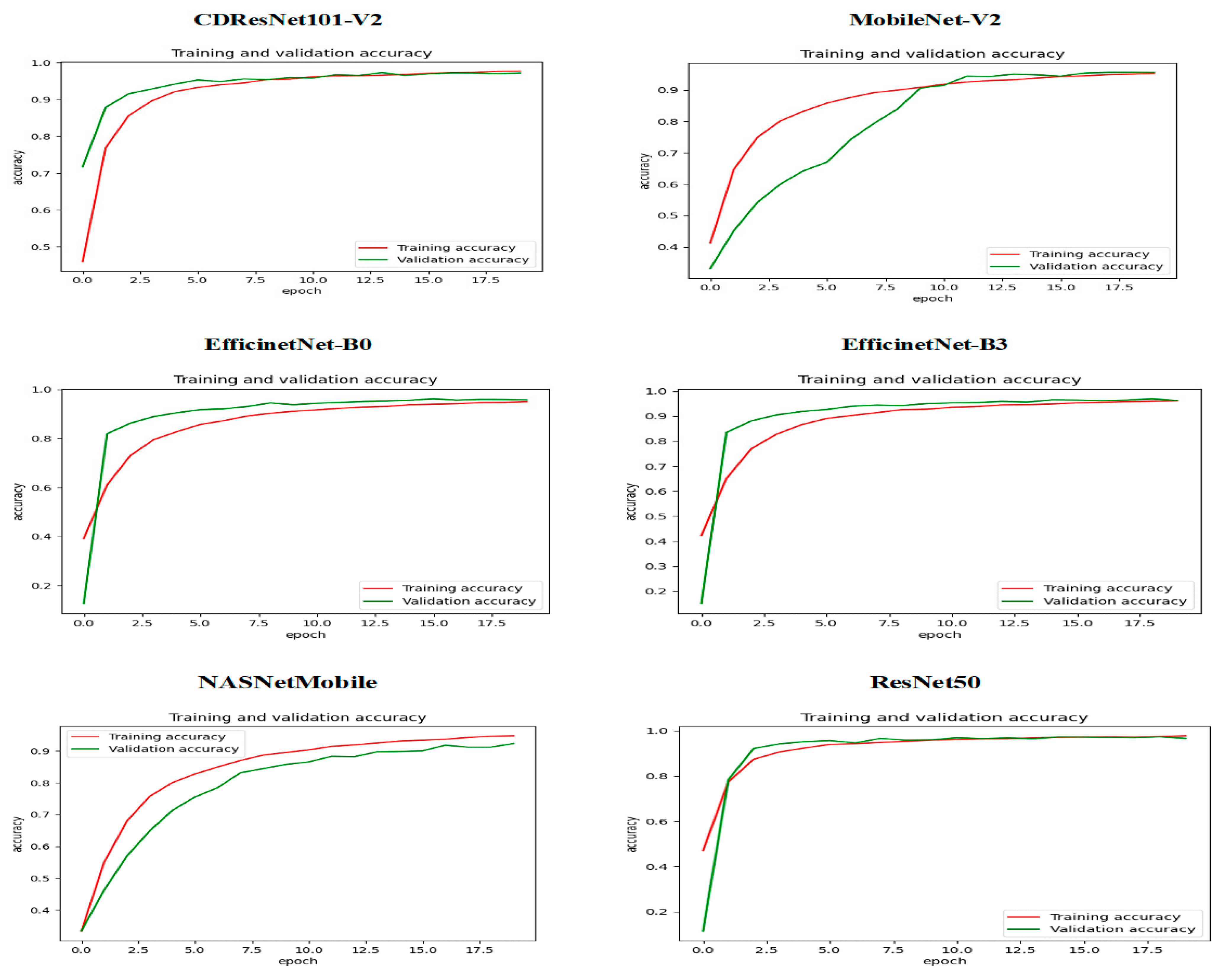Figure 19 displays the training and validation accuracy of six DL models across various epochs. The red line illustrates the training accuracy, while the green line shows the validation accuracy. For the CDResNet101-V2 model, the validation accuracy rose sharply at the beginning, surpassing the training accuracy in the early epochs. This phenomenon may be attributed to regularization effects or dropout techniques. As training continued, both accuracy metrics began to converge, suggesting effective model learning with minimal signs of overfitting. By the end of the training, the accuracy values for both training and validation were nearly identical, indicating a well-trained model with balanced performance.

In the case of MobileNet-V2, the training accuracy increased rapidly, exceeding 80% within the first five epochs. The validation accuracy followed a similar upward trend but was slightly behind. Around the 10th epoch, both the training and validation accuracies converged at approximately 90%. Following this point, there were only minor improvements, and both metrics stabilized, showing no signs of overfitting. This pattern suggested that the model achieved balanced and optimal performance on both training and validation datasets.

For EfficientNet-B0, EfficientNet-B3, and ResNet50, the validation accuracy also displayed a significant increase early on, outpacing the training accuracy within the first few epochs. Afterward, both metrics improved steadily, with training accuracy catching up to validation accuracy midway through the training process. By the later epochs, both the training and validation accuracies converged at high values, approaching 100%. This outcome indicated that the model learned effectively without significant overfitting, as the validation performance closely matched the training performance.

For NASNetMobile, as training progressed, the training accuracy exhibited a steady increase, reaching approximately 0.93 by the end of the 20th epoch. The validation accuracy also improved over time, but at a slower rate, achieving about 0.90. Initially, the training accuracy rose more rapidly than the validation accuracy, indicating that the model was proficient at identifying patterns in the training dataset. However, the gap between the two curves suggested a slight level of overfitting, as the training accuracy consistently exceeded the validation accuracy throughout the training process.

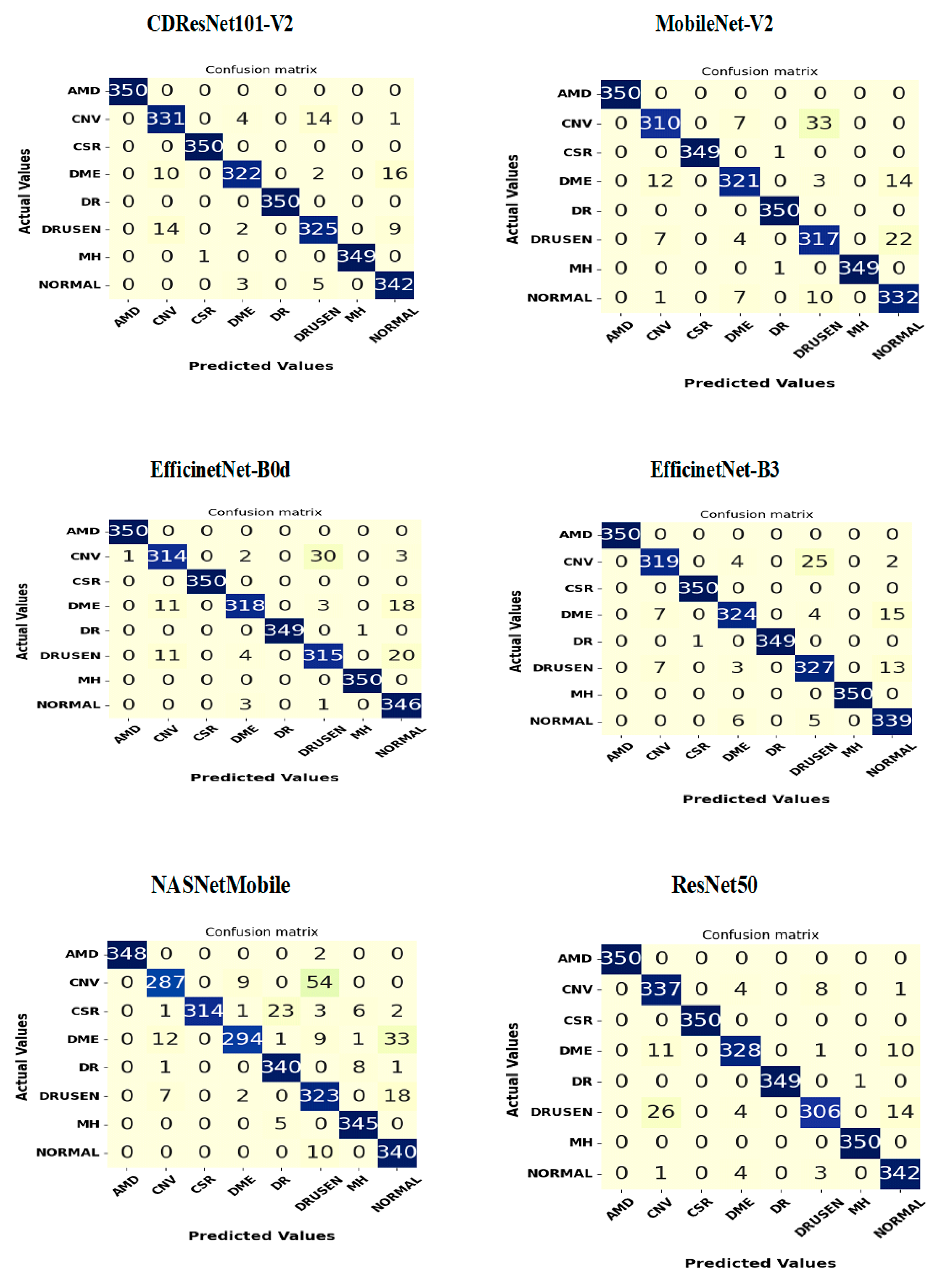
Figure 20 presents a confusion matrix for the six classification models, highlighting the relationship between actual and predicted class labels for the OCT-C8 test set of ED images. This test set consists of 2800 samples categorized into eight classes: AMD, CNV, CSR, DME, DR, drusen, MH, and normal, with each class containing 350 samples.

In the CDResNet101-V2 model, the diagonal entries of the classification matrix indicate the number of instances accurately classified for each category. There were 350 instances of AMD, CSR, and DR that were correctly identified as AMD, CSR, and DR, resulting in an accuracy of 100%. Additionally, 331 instances of CNV were accurately classified as CNV, achieving an accuracy of 94.5%. Furthermore, 322 instances of DME were correctly classified as DME, yielding an accuracy of 92%. For drusen, 325 instances were accurately classified, resulting in an accuracy of 92.85%. The model also correctly identified 349 instances of MH as MH, achieving an accuracy of 99.7%. Lastly, 342 instances of normal were correctly identified as normal, reaching an accuracy of 97.7%.

The off-diagonal entries in the matrix represent misclassifications. Specifically, 4 instances of CNV were incorrectly classified as DME, 14 as drusen, and 1 as normal. Additionally, 10 instances of DME were misidentified as CNV, while 16 instances of DME were mistakenly categorized as normal. These statistics highlight the model’s misclassifications and emphasize the classes that are often confused with one another. Overall, the model exhibited strong performance, with most categories showing high classification accuracy, though slight errors occurred for certain labels such as drusen and DME.

4.3. Statistical Analysis

To evaluate the dependability of CDResNet101-V2’s results, an extensive statistical examination was conducted. This examination focused on the confidence intervals. The confidence intervals of the six DL models are presented in

Table 9. The confidence intervals of the six DL models on the test set of the OCT-2017 dataset.

DL Model	Confidence Interval (%)
CDResNet101-V2	[99.82, 99.96]
MobileNet-V2	[99.38, 99.99]
EfficinetNet-B0	[99.26, 99.90]
EfficinetNet-B3	[94.67, 99.02]
NASNetMobile	[99.025, 99.94]
ResNet50	[99.28, 99.78]

and in Figure 21 for the first experiment and in

Table 10. The confidence intervals of the six DL models on the test set of the OCT-C8 dataset.

DL Model	Confidence Interval (%)
CDResNet101-V2	[98.78, 99.77]
MobileNet-V2	[98.15, 99.67]
EfficinetNet-B0	[98.35, 99.71]
EfficinetNet-B3	[98.60, 99.74]
NASNetMobile	[97.34, 98.92]
ResNet50	[98.65, 99.77]

and Figure 22 for the second experiment.

From Table 9, CDResNet101-V2 consistently exhibited the highest confidence interval range, with values between 99.82% and 99.96%, indicating exceptional performance with minimal variation. MobileNet-V2 demonstrated a confidence interval range of 99.38% to 99.99%. While the upper bound reached nearly 100%, the range was slightly wider than that of CDResNet101-V2, reflecting slightly more variability in predictions. EfficientNet-B0 showed a confidence interval range of 99.26% to 99.90%, reflecting strong performance but with a slightly lower upper bound compared to MobileNet-V2. EfficientNet-B3 had the widest range, spanning from 94.67% to 99.02%. This indicated relatively lower confidence compared to other models, with broader variability in predictions. NASNetMobile achieved a confidence interval range of 99.025% to 99.94%, demonstrating strong and consistent performance, though the lower bound was marginally below the top-performing models. ResNet50 exhibited a confidence interval range from 99.28% to 99.78%, showing solid performance with moderate variability.

In summary, CDResNet101-V2 emerged as the most reliable model based on its narrow and high confidence interval range, while EfficientNet-B3 displayed the most variability and lower bounds, suggesting room for improvement in its performance.

From Table 10, CDResNet101-V2 exhibited an impressive confidence interval ranging from 98.78% to 99.77%. It maintained high reliability with one of the narrowest and highest intervals, indicating consistent performance. MobileNet-V2 achieved a confidence interval range of 98.15% to 99.67%. While it demonstrated strong upper bound performance, its lower bound was slightly lower compared to other leading models, reflecting a bit more variability. EfficientNet-B0 showed a confidence interval range of 98.35% to 99.71%. It demonstrated robust performance with a relatively narrow range, indicating consistency. EfficientNet-B3 exhibited a confidence interval range of 98.60% to 99.74%. Its range was slightly narrower and higher than that of EfficientNet-B0, indicating marginally better reliability. NASNetMobile presented the widest confidence interval range, from 97.34% to 98.92%. This indicated a lower and more variable performance compared to other models, suggesting a need for improvement. ResNet50 achieved a confidence interval range of 98.65% to 99.77%. It matched the upper bound of CDResNet101-V2 and demonstrated strong reliability with a high and narrow range.

In summary, CDResNet101-V2 and ResNet50 distinguished themselves with exceptional upper bounds and narrow intervals, signifying highly consistent and reliable performance. Conversely, NASNetMobile exhibited the lowest and most variable range, highlighting its comparatively weaker consistency.

4.4. Ablation Study

An ablation study is a method used in DL to assess how different components or design choices of a model affect its performance. Researchers can evaluate the significance and contribution of these elements by systematically removing or changing specific components of the model.

The process begins with the complete model, which includes all components and optimizations. The performance of this model is measured using a test dataset. Next, one component is removed or altered at a time, and the model is retrained. The performance metrics of this modified model are then compared to the original baseline model to understand the impact of the removed or altered component. This process is repeated for all significant components within the model.

In the second experiment, we conducted an ablation analysis by modifying the optimizers and learning rate (LR) settings. We started with the Adam optimizer, applying an LR of 0.0001, which yielded an accuracy of 99.28%. Following this, we experimented with two additional optimizers: Stochastic Gradient Descent (SGD) and Root Mean Square Propagation (RMSprop). We tested LR values of 0.001, 0.0001, 0.00001, and 0.000001 for each optimizer. The results showcasing the accuracy of CDResNet101-V2 with various optimizers and LR values, are presented in

Table 11. CDResNet101-V2’s accuracies with three optimizers and four LR values.

	LR Value	Optimizer
CDResNet101-V2		Adam	SGD	RMSprop
	LR1 = 0.001	78.11%	99.1%	92.74
	LR2 = 0.0001	99.28%	98.3%	99.24
	LR3 = 0.00001	99.25%	93.12%	99.24
	LR4 = 0.000001	97.83%	80.63%	98.04

and depicted in Figure 23.

From the data in Table 11, we can observe the following performance metrics for various LR across different optimizers:

• For LR1 = 0.001, Adam achieved a performance of 78.11%, which is significantly lower than SGD at 99.1% and RMSprop at 92.74%.
• At LR2 = 0.0001, Adam showed an improvement, reaching the highest performance of 99.28%, slightly surpassing RMSprop at 99.24%, while SGD was marginally lower at 98.3%.
• With LR3 = 0.00001, Adam maintained a high performance of 99.25%, and RMSprop performed comparably at 99.24%, whereas SGD’s performance fell sharply to 93.12%.
• At LR4 = 0.000001, Adam’s performance decreased slightly to 97.83%. RMSprop also saw a decline to 98.04%, while SGD recorded the lowest performance at 80.63%.

In summary, Adam generally demonstrated strong performance across most learning rates, achieving the best result at LR2 (0.0001) with 99.28%. RMSprop was also effective, especially at LR2 and LR3. SGD performed well at the higher learning rates (LR1 and LR2) but showed a significant drop in performance at the lower learning rates (LR3 and LR4).

4.5. Visual Explanations via Gradient-Based Localization

Grad-CAM is a visualization technique used to visualize and interpret DL models, particularly CNNs. Created by Selvaraju et al. [42], Grad-CAM generates heatmaps for specific classes, showing which areas of an input image significantly influence the model’s decision-making. The process begins by calculating the gradients associated with a chosen class as they pass through the final convolutional layers of the CNN. These gradients are then averaged to assign a weight to each feature map, ultimately combining them into a weighted sum. After this, a ReLU (rectified linear unit) activation function is applied to focus on the positive contributions related to the target class. The resulting heatmap is overlaid on the original image, allowing users to visually identify the regions that are critical to the model’s classification decisions. Grad-CAM has been particularly useful in fields like medical imaging and autonomous driving, enhancing understanding of how models function and boosting confidence in AI systems. Figure 24 depicts Grad-CAM for EDs.

In the Grad-CAM visualizations for CNV, the heatmaps primarily emphasize the subretinal areas near the macula. This corresponds to the known location of neovascular membranes in the pathology of CNV. The model’s focus on this central region is consistent with clinical observations that CNV lesions usually develop beneath or near the fovea, resulting in leakage or bleeding. This indicates that the model is concentrating on areas that are relevant to the pathology rather than on non-informative regions. The attention also corresponds with the irregular appearance of abnormal blood vessels under the macula, which is a key diagnostic characteristic in CNV.

In cases of DME, the Grad-CAM heatmaps reveal widespread activation in the macular area. This corresponds to the thickening and fluid buildup around the fovea that is characteristic of DME. Such a pattern aligns with clinical observations, where retinal thickening is primarily centered at the macula but may extend unevenly based on the severity of the edema. The model’s focus indicates that it recognizes asymmetry in retinal thickness and leakage associated with DME. The heatmaps highlight areas of clinically significant macular thickening, which correspond to the typical diagnostic regions utilized by ophthalmologists.

Grad-CAM outputs for drusen indicate that attention is focused in the perifoveal region, which corresponds with the common distribution of drusen deposits found between the retinal pigment epithelium and Bruch’s membrane. These deposits produce irregular reflectivity patterns, mainly around the macula. The heatmap activations appear asymmetrical and spot-like, resembling the scattered distribution of drusen observed in the early and intermediate stages of age-related macular degeneration (AMD). The model’s attention aligns with the clinically significant topography of drusen deposits, highlighting its dependence on pathological markers.

In normal images, the Grad-CAM outputs show little to no focused attention across the retina, lacking significant hotspots in the macula or optic disc areas. This pattern of diffuse attention suggests that the model does not identify features indicative of pathology, aligning with the absence of asymmetrical abnormalities in healthy retinas. The absence of focused attention reinforces the model’s ability to differentiate between normal symmetry and pathological asymmetry.

The Grad-CAM outputs for all classes show focused attention that corresponds with clinically significant retinal asymmetries, which supports the model’s interpretability. This connection between the model’s focus and recognized pathological areas increases confidence in its decision-making for the automated classification of retinal diseases.

4.6. Comparing the Results with the Recent Literature

EDs such as glaucoma, diabetic retinopathy, and cataracts have a significant impact on visual health worldwide. These conditions are commonly diagnosed using fundus imaging; however, the manual analysis of these images can be time-consuming and prone to errors, highlighting the need for automated diagnostic systems. To address these limitations, this research introduced a two-dimensional single-channel CNN based on ResNet101-V2 for the detection of EDs. Additionally, the model employed Grad-CAM to emphasize the affected areas of the retina.

Two experiments were conducted using the OCT-2017 and OCT-C8 datasets. These experiments utilized transfer learning with six DL models that were pre-trained on ImageNet, with fine-tuning performed using the training sets from the OCT datasets. The proposed model demonstrated impressive performance in both the eight-class and four-class classification tasks. In the four-class task, the model achieved an accuracy of 99.90%, specificity of 99.93%, precision of 99.80%, recall of 99.79%, and F1-score of 99.79%. In the eight-class task, it reached an accuracy of 99.27%, specificity of 99.58%, precision of 97.13%, recall of 97.10%, and F1-score of 97.10%. This proposed model facilitates the early detection of eye diseases, thereby improving treatment outcomes and streamlining diagnostic processes, ultimately saving time and reducing costs.

The comparative analysis of the studies presented in

Table 12. Comparison of the proposed model’s results with recent models’ results.

Reference	Methodology	Evaluation Metrics	Dataset
Baba, S. et al. [24]	CNN	Accuracy: 98%	OCT-2017
Quek, T.C. et al. [25]	CNN-ViT	Accuracy: 94.98%	OCT-2017
Elkholy, M. et al. [26]	CNN and VGG16	Accuracy: 97%	OCT-2017
Wu, J. et al. [27]	RLMENet	MIoU of 86.55% and MPA of 98.73%	OCT-2017
Tsuji, T. et al. [28]	Capsule network	Accuracy: 99.6%	OCT-2017
He, J. et al. [29]	Swin-Poly Transformer network	Accuracy: 99.80%	OCT-2017
Hassan, E. et al. [30]	ResNet (50) and RF algorithms	Accuracy: 97.47%	OCT-2017
Laouarem, A. et al. [31]	CPTE	Accuracy: 99.40%	OCT-2017
Khalil, I. et al. [32]	OCTNet	Accuracy: 99.50%	OCT-2017
The proposed model	Two-dimensional single-channel CNN based on ResNet101-V2 and Grad-CAM	Accuracy: 99.90% and 99.27%	OCT-2017 and OCT-8

and

Table 13. Comparison of the proposed model’s metrics with recent models’ results.

Reference	Precision (%)	Recall (%)	F1-Score (%)
Baba, S. et al. [24]	95	100	97
He, J. et al. [29]	99.80	99.80	99.80
Hassan, E. et al. [30]	97.40	98.36	97.88
Khalil, I. et al. [32]	99.51	99.50	99.50
The proposed model	99.80	99.79	99.79

and Figure 25 shows the following results: Baba, S. et al. [24] used a CNN and achieved an accuracy of 98%. Quek, T.C. et al. [25] employed a CNN-ViT approach, reporting an accuracy of 94.98%. Elkholy, M. et al. [26] combined CNN and VGG16 models, reaching an accuracy of 97%. Wu, J. et al. [27] implemented RLMENet, which achieved a mean Intersection over Union (MIoU) of 86.55% and a Mean Pixel Accuracy (MPA) of 98.73%. Tsuji, T. et al. [28] adopted a capsule network, achieving an accuracy of 99.6%. He, J. et al. [29] developed a Swin-Poly Transformer network, obtaining an accuracy of 99.80%. Hassan, E. et al. [30] combined ResNet50 with RF algorithms, achieving an accuracy of 97.47%. Laouarem, A. et al. [31] used the CPTE method, achieving an accuracy of 99.40%. Khalil, I. et al. [32] proposed OCTNet, reporting an accuracy of 99.50%.

The highest accuracy of 99.90% was achieved by the proposed model, which incorporated advanced techniques such as Grad-CAM for improved localization and detection. The Swin-Poly Transformer networks developed by He, J. et al. [29] demonstrated strong performance with an accuracy of 99.80%, while the capsule networks from Tsuji, T. et al. [28] closely followed with an accuracy of 99.6%. Traditional CNN approaches, as seen in the works of Baba, S. et al. [24] and Elkholy, M. et al. [26], achieved lower accuracies of 98% and 97%, respectively. Other models like OCTNet and CPTE also performed well, with accuracies of 99.50% and 99.40%, indicating the effectiveness of specialized architectures. Overall, the proposed model outperformed its counterparts, underscoring the advantages of utilizing ResNet101-V2 with Grad-CAM for robust and interpretable ocular disease detection.

The OCT classification task features distinct localized lesions and extensive labeled datasets, enabling both a deep convolutional neural network (ResNet101 V2) and an advanced transformer model (Swin-Poly) to achieve nearly perfect separation. While the transformer benefits from multiscale attention and adaptive PolyLoss, providing slight advantages in robustness, both models exhibit similar performance due to their underlying feature learning capabilities. Although the results on the OCT-2017 dataset are comparable, the performance on the OCT-C8 dataset differs, with our model achieving higher accuracy than that of He, J. et al. [29].

5. Conclusions

In this research, we developed a two-dimensional single-channel CNN based on the ResNet101-V2 architecture, utilizing the capabilities of DNNs for the detection of EDs. Furthermore, our proposed model used the Grad-CAM technique to pinpoint specific areas impacted by GGOs associated with EDs. This model improved the early detection of EDs, facilitating timely interventions and enhancing patient outcomes, while also optimizing the diagnostic process to reduce time and costs for patients. We conducted two experiments utilizing the OCT-2017 and OCT-C8 datasets for multiclass classification tasks. In these experiments, we implemented transfer learning to pre-train six DL models: CDResNet101-V2, MobileNet-V2, EfficientNet-B0, EfficientNet-B3, NASNetMobile, and ResNet50. During the initial transfer learning phase, we conducted supervised pre-training using the ImageNet dataset for these six models. Following this, we performed the fine-tuning phase with the training sets from the two OCT datasets. The datasets underwent pre-processing through techniques such as data augmentation, resizing, and normalization to ensure consistent input. Our proposed DL model was compared against traditional classifiers. In the four-class classification task, our model achieved an accuracy of 99.90%, specificity of 99.93%, precision of 99.80%, recall of 99.79%, and F1-score of 99.79%. In the eight-class classification task, the model reached an accuracy of 99.27%, specificity of 99.58%, precision of 97.13%, recall of 97.10%, and F1-score of 97.10%. However, it is important to note that this research does not assess the response time of the proposed CAD method in a real-time environment, despite its high success rate in classifying EDs.

References

1. Chin, Y.H.; Ng, C.H.; Lee, M.H.; Koh, J.W.H.; Kiew, J.; Yang, S.P.; Sundar, G.; Khoo, C.M. Prevalence of Thyroid Eye Disease in Graves’ Disease: A Meta-analysis and Systematic Review. Clin. Endocrinol. 2020, 93, 363–374. [Google Scholar] [CrossRef] [PubMed]
2. Al-Aswad, L.A.; Elgin, C.Y.; Patel, V.; Popplewell, D.; Gopal, K.; Gong, D.; Thomas, Z.; Joiner, D.; Chu, C.-K.; Walters, S.; et al. Real-Time Mobile Teleophthalmology for the Detection of Eye Disease in Minorities and Low Socioeconomics At-Risk Populations. Asia-Pac. J. Ophthalmol. 2021, 10, 461–472. [Google Scholar] [CrossRef]
3. Sarki, R.; Ahmed, K.; Wang, H.; Zhang, Y. Automated Detection of Mild and Multi-Class Diabetic Eye Diseases Using Deep Learning. Health Inf. Sci. Syst. 2020, 8, 32. [Google Scholar] [CrossRef] [PubMed]
4. Kermany, D.S.; Goldbaum, M.; Cai, W.; Valentim, C.C.S.; Liang, H.; Baxter, S.L.; McKeown, A.; Yang, G.; Wu, X.; Yan, F.; et al. Identifying Medical Diagnoses and Treatable Diseases by Image-Based Deep Learning. Cell 2018, 172, 1122–1131.e9. [Google Scholar] [CrossRef]
5. WHO Report. Available online: https://www.who.int/news-room/fact-sheets/detail/blindness-and-visual-impairment (accessed on 10 August 2023).
6. Steinmetz, J.D.; Bourne, R.R.A.; Briant, P.S.; Flaxman, S.R.; Taylor, H.R.B.; Jonas, J.B.; Abdoli, A.A.; Abrha, W.A.; Abualhasan, A.; Abu-Gharbieh, E.G.; et al. Causes of Blindness and Vision Impairment in 2020 and Trends over 30 Years, and Prevalence of Avoidable Blindness in Relation to VISION 2020: The Right to Sight: An Analysis for the Global Burden of Disease Study. Lancet Glob. Health 2021, 9, e144–e160. [Google Scholar] [CrossRef] [PubMed]
7. Katibeh, M.; Pakravan, M.; Yaseri, M.; Pakbin, M.; Soleimanizad, R. Prevalence and Causes of Visual Impairment and Blindness in Central Iran; The Yazd Eye Study. J. Ophthalmic Vis. Res. 2015, 10, 279. [Google Scholar] [CrossRef]
8. Paudel, P.; Ramson, P.; Naduvilath, T.; Wilson, D.; Phuong, H.T.; Ho, S.M.; Giap, N.V. Prevalence of Vision Impairment and Refractive Error in School Children in B a R Ia—V Ung T Au Province, V Ietnam. Clin. Exper Ophthalmol. 2014, 42, 217–226. [Google Scholar] [CrossRef]
9. Edussuriya, K.; Sennanayake, S.; Senaratne, T.; Marshall, D.; Sullivan, T.; Selva, D.; Casson, R.J. The Prevalence and Causes of Visual Impairment in Central Sri Lanka. Ophthalmology 2009, 116, 52–56. [Google Scholar] [CrossRef]
10. Tong, Y.; Lu, W.; Yu, Y.; Shen, Y. Application of Machine Learning in Ophthalmic Imaging Modalities. Eye Vis. 2020, 7, 22. [Google Scholar] [CrossRef]
11. Balyen, L.; Peto, T. Promising Artificial Intelligence-Machine Learning-Deep Learning Algorithms in Ophthalmology. Asia Pac. J. Ophthalmol. 2019, 8, 264–272. [Google Scholar] [CrossRef]
12. Alqudah, A.M. AOCT-NET: A Convolutional Network Automated Classification of Multiclass Retinal Diseases Using Spectral-Domain Optical Coherence Tomography Images. Med. Biol. Eng. Comput. 2020, 58, 41–53. [Google Scholar] [CrossRef]
13. Li, T.; Bo, W.; Hu, C.; Kang, H.; Liu, H.; Wang, K.; Fu, H. Applications of Deep Learning in Fundus Images: A Review. Med. Image Anal. 2021, 69, 101971. [Google Scholar] [CrossRef] [PubMed]
14. Grassmann, F.; Mengelkamp, J.; Brandl, C.; Harsch, S.; Zimmermann, M.E.; Linkohr, B.; Peters, A.; Heid, I.M.; Palm, C.; Weber, B.H.F. A Deep Learning Algorithm for Prediction of Age-Related Eye Disease Study Severity Scale for Age-Related Macular Degeneration from Color Fundus Photography. Ophthalmology 2018, 125, 1410–1420. [Google Scholar] [CrossRef] [PubMed]
15. Lin, W.-C.; Chen, J.S.; Chiang, M.F.; Hribar, M.R. Applications of Artificial Intelligence to Electronic Health Record Data in Ophthalmology. Trans. Vis. Sci. Technol. 2020, 9, 13. [Google Scholar] [CrossRef]
16. An, G.; Omodaka, K.; Hashimoto, K.; Tsuda, S.; Shiga, Y.; Takada, N.; Kikawa, T.; Yokota, H.; Akiba, M.; Nakazawa, T. Glaucoma Diagnosis with Machine Learning Based on Optical Coherence Tomography and Color Fundus Images. J. Healthc. Eng. 2019, 2019, 4061313. [Google Scholar] [CrossRef]
17. Ting, D.S.W.; Peng, L.; Varadarajan, A.V.; Keane, P.A.; Burlina, P.M.; Chiang, M.F.; Schmetterer, L.; Pasquale, L.R.; Bressler, N.M.; Webster, D.R.; et al. Deep Learning in Ophthalmology: The Technical and Clinical Considerations. Prog. Retin. Eye Res. 2019, 72, 100759. [Google Scholar] [CrossRef] [PubMed]
18. Soomro, T.A.; Afifi, A.J.; Zheng, L.; Soomro, S.; Gao, J.; Hellwich, O.; Paul, M. Deep Learning Models for Retinal Blood Vessels Segmentation: A Review. IEEE Access 2019, 7, 71696–71717. [Google Scholar] [CrossRef]
19. Sengupta, S.; Singh, A.; Leopold, H.A.; Gulati, T.; Lakshminarayanan, V. Ophthalmic Diagnosis Using Deep Learning with Fundus Images—A Critical Review. Artif. Intell. Med. 2020, 102, 101758. [Google Scholar] [CrossRef]
20. Sreng, S.; Maneerat, N.; Hamamoto, K.; Win, K.Y. Deep Learning for Optic Disc Segmentation and Glaucoma Diagnosis on Retinal Images. Appl. Sci. 2020, 10, 4916. [Google Scholar] [CrossRef]
21. Guo, Y.; Liu, Y.; Oerlemans, A.; Lao, S.; Wu, S.; Lew, M.S. Deep Learning for Visual Understanding: A Review. Neurocomputing 2016, 187, 27–48. [Google Scholar] [CrossRef]
22. Liu, W.; Wang, Z.; Liu, X.; Zeng, N.; Liu, Y.; Alsaadi, F.E. A Survey of Deep Neural Network Architectures and Their Applications. Neurocomputing 2017, 234, 11–26. [Google Scholar] [CrossRef]
23. Cireşan, D.; Meier, U.; Schmidhuber, J. Multi-Column Deep Neural Networks for Image Classification. In Proceedings of the 2012 IEEE Conference on Computer Vision and Pattern Recognition, Providence, RI, USA, 16–21 June 2012. [Google Scholar] [CrossRef]
24. Baba, S.; Kumari, P.; Saxena, P. Retinal Disease Classification Using Custom CNN Model From OCT Images. Procedia Comput. Sci. 2024, 235, 3142–3152. [Google Scholar] [CrossRef]
25. Quek, T.C.; Takahashi, K.; Kang, H.G.; Thakur, S.; Deshmukh, M.; Tseng, R.M.W.W.; Nguyen, H.; Tham, Y.-C.; Rim, T.H.; Kim, S.S.; et al. Predictive, Preventive, and Personalized Management of Retinal Fluid via Computer-Aided Detection App for Optical Coherence Tomography Scans. EPMA J. 2022, 13, 547–560. [Google Scholar] [CrossRef]
26. Elkholy, M.; Marzouk, M.A. Deep Learning-Based Classification of Eye Diseases Using Convolutional Neural Network for OCT Images. Front. Comput. Sci. 2024, 5, 1252295. [Google Scholar] [CrossRef]
27. Wu, J.; Liu, S.; Xiao, Z.; Zhang, F.; Geng, L. Joint Segmentation of Retinal Layers and Macular Edema in Optical Coherence Tomography Scans Based on RLMENet. Med. Phys. 2022, 49, 7150–7166. [Google Scholar] [CrossRef]
28. Tsuji, T.; Hirose, Y.; Fujimori, K.; Hirose, T.; Oyama, A.; Saikawa, Y.; Mimura, T.; Shiraishi, K.; Kobayashi, T.; Mizota, A.; et al. Classification of Optical Coherence Tomography Images Using a Capsule Network. BMC Ophthalmol. 2020, 20, 114. [Google Scholar] [CrossRef]
29. He, J.; Wang, J.; Han, Z.; Ma, J.; Wang, C.; Qi, M. An Interpretable Transformer Network for the Retinal Disease Classification Using Optical Coherence Tomography. Sci. Rep. 2023, 13, 3637. [Google Scholar] [CrossRef]
30. Hassan, E.; Elmougy, S.; Ibraheem, M.R.; Hossain, M.S.; AlMutib, K.; Ghoneim, A.; AlQahtani, S.A.; Talaat, F.M. Enhanced Deep Learning Model for Classification of Retinal Optical Coherence Tomography Images. Sensors 2023, 23, 5393. [Google Scholar] [CrossRef] [PubMed]
31. Laouarem, A.; Kara-Mohamed, C.; Bourennane, E.-B.; Hamdi-Cherif, A. HTC-Retina: A Hybrid Retinal Diseases Classification Model Using Transformer-Convolutional Neural Network from Optical Coherence Tomography Images. Comput. Biol. Med. 2024, 178, 108726. [Google Scholar] [CrossRef]
32. Khalil, I.; Mehmood, A.; Kim, H.; Kim, J. OCTNet: A Modified Multi-Scale Attention Feature Fusion Network with InceptionV3 for Retinal OCT Image Classification. Mathematics 2024, 12, 3003. [Google Scholar] [CrossRef]
33. Available online: https://www.kaggle.com/datasets/paultimothymooney/kermany2018 (accessed on 1 June 2018).
34. Naren, O.S. Retinal OCT Image Classification-C8; Kaggle: 2022. Available online: https://www.kaggle.com/datasets/obulisainaren/retinal-oct-c8 (accessed on 4 August 2022).
35. He, K.; Zhang, X.; Ren, S.; Sun, J. Identity Mappings in Deep Residual Networks. arXiv 2016, arXiv:1603.05027. [Google Scholar]
36. He, K.; Zhang, X.; Ren, S.; Sun, J. Delving Deep into Rectifiers: Surpassing Human-Level Performance on Imagenet Classification. arXiv 2015, arXiv:1502.01852. [Google Scholar]
37. Sandler, M.; Howard, A.; Zhu, M.; Zhmoginov, A.; Chen, L.-C. MobileNetV2: Inverted Residuals and Linear Bottlenecks. In Proceedings of the 2018 IEEE/CVF Conference on Computer Vision and Pattern Recognition, Salt Lake City, UT, USA, 18–23 June 2018; IEEE: Piscataway, NJ, USA, 2018; pp. 4510–4520. [Google Scholar]
38. Tan, M.; Le, Q.V. EfficientNet: Rethinking Model Scaling for Convolutional Neural Networks. arXiv 2019, arXiv:1905.11946. [Google Scholar] [CrossRef]
39. Zoph, B.; Vasudevan, V.; Shlens, J.; Le, Q.V. Learning Transferable Architectures for Scalable Image Recognition. In Proceedings of the IEEE Conference On Computer Vision And Pattern Recognition, Honolulu, HI, USA, 21–26 July 2017. [Google Scholar]
40. Radhika, K.; Devika, K.; Aswathi, T.; Sreevidya, P.; Sowmya, V.; Soman, K.P. Performance Analysis of NASNet on Unconstrained Ear Recognition. In Nature Inspired Computing for Data Science; Rout, M., Rout, J.K., Das, H., Eds.; Studies in Computational Intelligence; Springer International Publishing: Cham, Switzerland, 2020; Volume 871, pp. 57–82. ISBN 978-3-030-33819-0. [Google Scholar]
41. He, K.; Zhang, X.; Ren, S.; Sun, J. Deep Residual Learning for Image Recognition. In Proceedings of the IEEE Conference on Computer Vision and Pattern Recognition, Boston, MA, USA, 7–12 June 2015. [Google Scholar]
42. Selvaraju, R.R.; Cogswell, M.; Das, A.; Vedantam, R.; Parikh, D.; Batra, D. Grad-CAM: Visual Explanations from Deep Networks via Gradient-Based Localization. arXiv 2016, arXiv:1610.02391. [Google Scholar] [CrossRef]
Figure 1. Fundus disorders [4].
Symmetry 17 00768 g001
Figure 2. Various samples from OCT-2017.
Symmetry 17 00768 g002
Figure 3. The training set distribution.
Symmetry 17 00768 g003
Figure 4. The test set distribution.
Symmetry 17 00768 g004
Figure 5. Various samples from OCT-C8.
Symmetry 17 00768 g005
Figure 6. The proposed model architecture.
Symmetry 17 00768 g006
Figure 7. CDResNet101-V2 architecture.
Symmetry 17 00768 g007
Figure 8. ResNet101-V2 architecture.
Symmetry 17 00768 g008
Figure 9. Residual block architecture.
Symmetry 17 00768 g009
Figure 10. EfficientNet-B3 architecture.
Symmetry 17 00768 g010
Figure 11. A performance comparison between the six DL models’ results on the OCT-2017 dataset.
Symmetry 17 00768 g011
Figure 12. The class-wise results of CDResNet101-V2 on the OCT-2017 dataset.
Symmetry 17 00768 g012
Figure 13. The training vs. validation loss of the six DL models on the OCT-2017 dataset.
Symmetry 17 00768 g013
Figure 14. The training vs. validation accuracy of the six DL models on the OCT-2017 dataset.
Symmetry 17 00768 g014
Figure 15. The confusion matrices of the six DL models on the test set of the OCT-2017 dataset.
Symmetry 17 00768 g015
Figure 16. A performance comparison between the six DL models’ results on the OCT-C8 dataset.
Symmetry 17 00768 g016
Figure 17. The class-wise result of CDResNet101-V2 on the OCT-C8 dataset.
Symmetry 17 00768 g017
Figure 18. The training vs. validation loss of the six DL models on the OCT-C8dataset.
Symmetry 17 00768 g018
Figure 19. The training vs. validation accuracy of the six DL models on the OCT-C8 dataset.
Symmetry 17 00768 g019
Figure 20. The confusion matrices of the six DL model on the test set of the OCT-C8 dataset.
Symmetry 17 00768 g020
Figure 21. The confidence intervals of the six DL models on the test set of the OCT-2017 dataset.
Symmetry 17 00768 g021
Figure 22. The confidence intervals of the six DL models on the test set of the OCT-C8 dataset.
Symmetry 17 00768 g022
Figure 23. CDResNet101-V2’s accuracies with three optimizers and three LR values.
Symmetry 17 00768 g023
Figure 24. Grad-CAM for EDs.
Symmetry 17 00768 g024
Figure 25. Comparison of the proposed model’s metrics with recent models’ results of [24,29,30,32].
Symmetry 17 00768 g025