Stochastic Programming-Based Annual Peak-Regulation Potential Assessing Method for Virtual Power Plants

Abstract

The intervention of distributed loads, propelled by the swift advancement of distributed energy sources and the escalating demand for diverse load types encompassing electricity and cooling within virtual power plants (VPPs), has exerted an influence on the symmetry of the grid. Consequently, a quantitative assessment of the annual peak-shaving capability of a VPP is instrumental in mitigating the peak-to-valley difference in the grid, enhancing the operational safety of the grid, and reducing grid asymmetry. This paper presents a peak-shaving optimization method for VPPs, which takes into account renewable energy uncertainty and flexible load demand response. Firstly, wind power (WP), photovoltaic (PV) generation, and demand-side response (DR) are integrated into the VPP framework. Uncertainties related to WP and PV generation are incorporated through the scenario method within deterministic constraints. Secondly, a stochastic programming (SP) model is established for the VPP, with the objective of maximizing the peak-regulation effect and minimizing electricity loss for demand-side users. The case study results indicate that the proposed model effectively tackles peak-regulation optimization across diverse new energy output scenarios and accurately assesses the peak-regulation potential of the power system. Specifically, the proportion of load decrease during peak hours is 18.61%, while the proportion of load increase during off-peak hours is 17.92%. The electricity loss degrees for users are merely 0.209 in summer and 0.167 in winter, respectively.

1. Introduction

1.1. Background

In recent years, grid peak regulation has become prominent due to rapid electricity load growth. Amid fossil energy constraints, new energy generation is booming. However, the large-scale integration of new energy, characterized by fluctuation and randomness, exacerbates power system instability and grid load fluctuations, affecting grid symmetry. Addressing new energy output uncertainty is a major challenge for power system dispatch optimization. Additionally, demand response is crucial in reducing grid load fluctuations.

1.2. Recent Works

In grid peak shaving, DR guides users to optimize electricity consumption, offering high flexibility and response potential. DR reduces or delays user demand, influencing the supply–demand balance and alleviating system issues [1,2]. Reference [3] assesses DR techniques’ impact on enhancing building energy flexibility and management, using a heat pump system as a case study. Reference [4] introduces real-time pricing and demand response, enhancing peak-shaving potential in distributed networks and highlighting DR’s role in grid optimization. Reference [5] demonstrates the peak-shaving potential of actively controlled heat pump systems in DR, reducing peak load, promoting renewable self-consumption, and enhancing grid reliability. Reference [6] explores peer-to-peer trading and shared storage among industrial buildings, promoting DR, reducing peak demand, and improving energy efficiency. Reference [7] investigates the economic feasibility of peak shaving and DR with energy storage in residential sectors, showing cost reductions through strategic technology and capacity choices.

Furthermore, VPPs aggregate distributed energy and demand-side resources, participating in the electricity market as a unified entity for coordinated dispatch and management. Studies on VPP optimization considering demand response include the following: Reference [8] explores coordinated strategies for VPP clusters, enhancing peak shaving and reducing costs through flexible mechanisms. Reference [9] aggregates various energy sources into a VPP, considering multiple costs for day-ahead dispatch modeling. Reference [10] applies a data-mining-based incentive scheme in VPPs, adaptively determining optimal rates for consumers. Reference [11] studies the impact of integrating diverse resources into a VPP, encouraging active demand-side participation. Reference [12] proposes a multi-VPP electricity–carbon interaction model, considering integrated demand response and user satisfaction. Reference [13] introduces a multi-market model, converting fixed prices into dynamic ones to enhance demand response effectiveness, optimizing for both market theory and consumer satisfaction. These studies highlight the importance of VPPs in integrating resources for power system regulation.

However, in day-ahead power dispatch planning, many studies use a deterministic mode that treats forecasted renewable energy as planned values, relying heavily on forecast accuracy. Deviations can affect peak-shaving stability and make assessing potential difficult. To tackle energy-side output uncertainty, scholars propose robust optimization (RO), chance-constrained programming, and scenario-based methods. Distributionally RO optimizes under the worst-case scenario by constructing ambiguous sets for uncertain probabilities. Reference [14] uses a Wasserstein distance approach to mitigate conservatism, while reference [15] applies data-driven methods to handle battery and market uncertainties. Chance-constrained programming permits some constraint violation but ensures a minimum satisfaction level, as demonstrated in reference [16] for renewable and demand uncertainties, and in reference [17] for integrated energy network models. The scenario method samples error scenarios from assumed distributions; reference [18] uses seasonal autoregressive models for battery, EV, and PV uncertainties, reference [19] employs two-stage SP with k-means clustering, and reference [20] generates scenarios from probability density functions for wind and solar uncertainties. These studies highlight the importance of considering energy-side uncertainty and leveraging demand-side resources in VPPs for power system optimization.

Existing research progress is systematically summarized and categorized into three key aspects, demand response strategies, VPP optimization approaches, and uncertainty management considerations, as comprehensively detailed in

Table 1. Summary of state-of-the-art methods.

	Fields	Contributions
Demand Response	Thermal flexibility	Heat pump flexibility potential assessed [3] Peak-shaving participation studied [5]
	Dynamic pricing	Distribution network peak shaving via pricing [4]
	Energy storage	Industrial storage sharing proposed [6] Residential storage economics analyzed [7]
VPP	Cluster operation	Multi-VPP cost–potential optimization modeled [8]
	Energy aggregation	Renewable–storage–pumped hydro coordination [9] Gas turbine integration studied [11]
	Incentive design	Adaptive pricing schemes developed [10]
	Integrated dispatch	Electricity–carbon–user satisfaction model [12]
	Pricing strategy	Dynamic pricing–satisfaction framework [13]
Uncertainty Management	Robust optimization	Wasserstein-based DRO method developed [14]
	Chance constraints	Probabilistic constraints applied [16,17]
	Scenario generation	Renewable-load uncertainty scenarios created [18,19,20]

.

1.3. Motivations and Contributions

Most of the existing methods facilitate the integration of distributed energy and flexible load resources into VPPs for grid optimization, primarily focusing on distributed and autonomous flexible loads. However, large-scale logistics parks are yet to be involved in VPP optimization for peak shaving and potential assessment due to several reasons:

(1) The significant electricity consumption and temperature sensitivity of office and cold storage facilities in logistics parks can lead to large temperature deviations during peak shaving, necessitating a reasonable mathematical model.

(2) There is currently no annual peak-shaving-potential assessment method for VPPs that incorporates demand-side response from large-scale cold storage.

(3) The increasing penetration of renewable energy and the unpredictability of new energy sources, coupled with the strong randomness of system load fluctuations, exacerbates the challenge of peak shaving for cooling facilities and the difficulty of assessing peak-shaving potential.

To address these challenges, this paper models the uncertainty of wind and photovoltaic output using a time-series probabilistic scenario set. It proposes a VPP peak-shaving optimization method that accounts for new energy uncertainty and flexible load demand response and evaluates its annual peak-shaving capability. Specifically, (1) electric-cooling coupled flexible loads are integrated into VPPs for grid demand-side management, which aggregates uncertain distributed energy resources. This coordination leverages load inertia to mitigate renewable fluctuations, reducing curtailment and net load peak-valley differences. (2) A novel UELD index combining thermal comfort and sales pressure is developed to quantify adjustment losses, generating Pareto-optimal solutions balancing peak-shaving efficacy and economic impacts. (3) Stochastic programming simulates annual renewable scenarios, with the dual objectives of peak-shaving optimization and UELD minimization. Seasonal load/renewable distributions are analyzed to determine annual potential, revealing temporal operational characteristics.

This paper is structured as follows: Section 1 introduces the research background and focus. Section 2 outlines the basic structure and modeling of the VPP. Section 3 addresses the treatment of renewable energy uncertainty, transforming it into a deterministic constraint. Section 4 develops a SP model for VPP peak regulation, incorporating DR. Section 5 presents case studies and compares the proposed method with other optimization approaches. Section 6 concludes the paper.

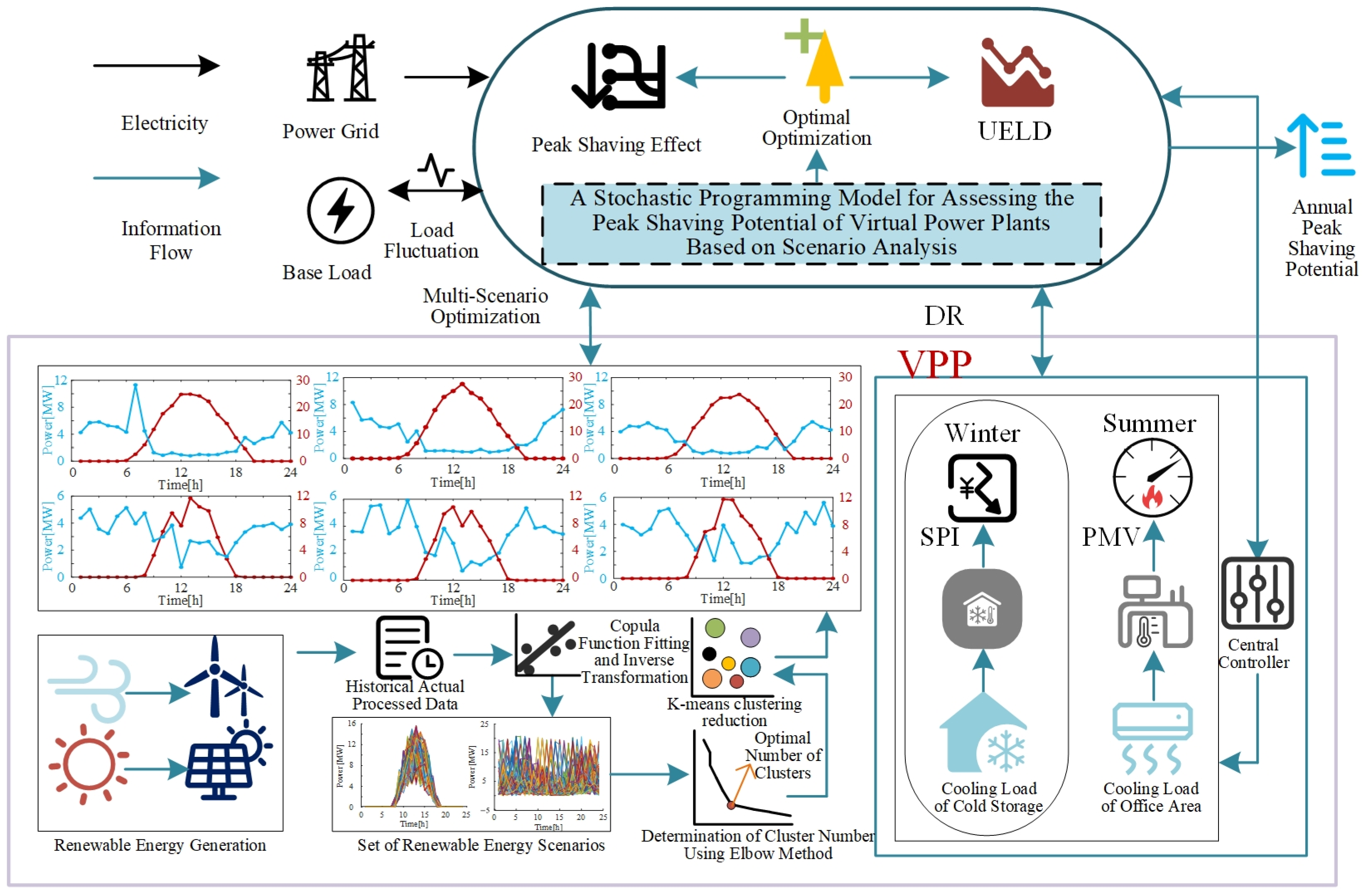
2. Basic Structure of the VPP

Total Framework with Diverse Cooling Loads

In this work, a WP plant, PV, and DR systems are aggregated into a VPP. The basic structure of a VPP is as shown in Figure 1.

As shown above, the day-ahead dispatch market is used as the analysis market. In the VPP, the WPP and PV power generation are used to meet the load demand. DR changes the electricity consumption behavior to achieve peak shaving and valley filling: When the net system load is at the trough, the VPP central control system increases the electricity purchase so that the chillers increase electricity consumption to fill the valley; when the net system load is at the peak, the VPP central control system reduces the electricity purchase so that the chillers reduce electricity consumption to achieve peak shaving. By considering the uncertainty of new energy power generation, the VPP operator develops a reasonable day-ahead power purchase plan. While performing system peak shaving and valley filling, it also considers the adverse impact of users’ DR and considers the DR plan. The degree of loss is minimized, and the grid peak-regulation effect is optimized. Finally, the annual peak-shaving potential of the virtual power plant is evaluated based on the optimization results.

3. Scene Construction Considering Scenery Uncertainty and Correlation

Because WP comes from wind energy while PV power generation depends on solar energy, these two new energy sources are spatially correlated in the same geographic area. In addition, wind speed and light intensity are simultaneously affected by meteorological conditions and seasonal variations; wind energy and solar energy are also correlated. Therefore, there is a nonnegligible spatiotemporal correlation between WP and PV power generation. To assess the impact of new energy generation on the power system more accurately, it is necessary to consider the stochasticity and correlation of new energy outputs.

In this work, first, the ksdensity function in the MATLAB 2018b toolbox is used to estimate the cumulative probability distributions of the historical WP and PV output data, and the cumulative distribution functions of the WP and the PV output are obtained. Next, to analyze the correlation of the WP output accurately, the selection can be considered at the same time. The Frank copula function between the nonnegative and negative correlations between variables was used to weigh the correlation and construct the joint distribution function [21]. Furthermore, the joint probability distribution function was sampled for each time period, and the specified numbers of WP output and PV output samples were obtained through the inverse transformation of the joint probability density function. Finally, to extract a representative scene from the numerous generated samples in the representative typical scenario, the optimal number of clusters was determined by calculating the sum of squared errors (SSE) under different numbers of clusters [22]. The K-means clustering method is used to perform cluster reduction on the generated scenes to obtain representative typical scenes.

3.1. Density Estimation

In this work, we use the MATLAB 2018b tool ksdensity function. The cumulative probability distribution is estimated on the historical data to obtain the cumulative distribution functions of the WP and the PV output $u_{WT}$ and $v_{PV}$.

3.2. Calculation of the Joint Distribution Function of Scenery

According to the cumulative distribution function obtained from $u_{WT}$ and $v_{PV}$ via Equation (1), the Frank copula function $C\left(u_{WT},v_{PV}\right)$ is used to establish a joint distribution function of the wind and power outputs for each period:

$$C(u,v)=-{\displaystyle \frac{1}{\theta }}\ln (1+{\displaystyle \frac{(e^{-\theta u}-1)(e^{-\theta v}-1)}{e^{-\theta }-1}})$$

(1)

where θ is a dependent parameter of the copula function; $u_{WT}$ and $v_{PV}$ are the cumulative distribution functions of the WP and PV outputs, respectively; and the sign and magnitude of the parameter θ determine the degree and type of dependence among the variables.

3.3. K-Means Clustering Reduction

The K-means clustering algorithm is a widely adopted method for data clustering [23]. It enables the dataset to be partitioned into multiple clusters, where data points within the same cluster exhibit proximity to one another, whereas those in different clusters demonstrate significant dissimilarity. This algorithm is employed to aggregate solar and wind output data, facilitating class analysis that precisely groups samples with high similarity into the same category and separates those with low similarity into distinct categories, thereby achieving effective data segmentation and classification.

In fact, several commonly used clustering methods include the following. (1) Hierarchical clustering: constructs dendrograms by calculating inter-sample distances, supporting bottom-up or top-down clustering, suitable for exploratory data analysis. (2) Density-based clustering: defines clusters through core point density reachability, automatically filtering noise points, with strong robustness to outliers. (3) Spectral Clustering: performs clustering after dimensionality reduction using eigenvectors of data similarity matrices, excelling at capturing complex manifold structures. (4) Subspace Clustering: identifies cluster structures in different feature subspaces, demonstrating significant advantages in handling high-dimensional data.

In this study, our objective is solely to integrate and classify annual renewable energy output data, without addressing outlier processing or ultra-high-dimensional data. Therefore, the straightforward K-means algorithm sufficiently meets the requirements.

To ensure the uniqueness of clustering results for the combined wind output data, this paper utilizes the elbow method [24]. This method is based on determining the optimal number of clusters for the wind and wind joint output scenario. The underlying principle is as follows: When k is less than the true number of clusters, an increase in k results in a substantial decrease in the sum of squared errors (SSE). As k approaches the actual number of clusters, the marginal gain in aggregation degree diminishes rapidly, leading to a sharp decline in the rate of SSE reduction. Subsequently, this rate stabilizes as k continues to increase. Consequently, the relationship between SSE and k forms an elbow shape, and the k value corresponding to the elbow represents the optimal number of clusters for the data. The step of the elbow method is as follows:

Step 1: For a sampled dataset of size n, iteratively calculate the values from 1 to the maximum number of Clusters k, and after each clustering, calculate the sum of squares of the distance from each point to the cluster center to which it belongs. The calculation formula is as follows:

$$SSE={\displaystyle \sum _{\mathrm{i}=1}^k{\displaystyle \sum _{p\in C_i}{\left|p-{\mu }_i\right|}^2}}$$

(2)

where k is the number of clusters obtained by clustering, $C_i$ is the set of the i-th cluster, p represents the data points in the cluster, and ${\mu }_i$ represents the centroid of the i-th cluster.

Step 2: Record the curve of the variation in the SSE value versus the number of clusters, find the point corresponding to the maximum value of the second-order difference as the elbow point, and determine it as the optimal number of clusters N. Thus, the clustering result of the joint output of wind and sun data corresponding to the optimal number of clusters determined by the elbow method is as follows:

$$\gamma =(l_1,l_2,\cdots ,l_N)$$

(3)

where N is the optimal number of clusters determined via the elbow method and where $\left(l_1{,l}_2,\cdots ,l_N\right)$ is the clustering result of the corresponding joint WP output data.

Step 3: Let the dataset be $X=\left(x_1{,x}_2,\cdots ,x_n\right)$. The cluster center determined in step 2 is $\mu =\left\{{\mu }_1{,\mu }_2,\cdots ,{\mu }_N\right\}$; each data point $x_j$ and cluster center ${\mu }_i$ are calculated, as is the distance $D_j$ between them, and then, each sample is assigned to the nearest cluster center. The calculation formula for $D_j$ is as follows (4):

$$D_j=\parallel x_{\beta }-{\mu }_j\parallel j=1,2,\cdots ,N \beta =1,2,\cdots ,\mathrm{n}$$

(4)

where $x_{\beta }$ is the no. $\beta$ data point; ${\mu }_j$ is the center of the j-th cluster; and N is the number of scenes.

Step 4: Constantly update the clustering centers, where the center $C_i$ of the i-th cluster is

$$C_i={\displaystyle \frac{1}{N_i}}{\displaystyle \sum _{h=1}^{N_i}{S}_{h,i}}$$

(5)

where $S_{h,i}$ is the h-th object in the i-th cluster and where $N_i$ is the number of objects in the i-th cluster.

Step 5: Repeat steps 3 and 4 until there is no significant change in the cluster centers.

4. Stochastic Programming Model of a Multi-Scenario-Based VPP

Due to the inherent uncertainty and stochastic nature of wind and PV outputs, traditional deterministic methods for predicting these outputs have limitations and struggle to account for various possibilities. In this paper, we employ a multi-scenario SP approach to simulate the impacts of wind and PV outputs. With the daily power purchase plan as the decision variable and the optimization of the comprehensive expectation as the objective, we establish a VPP peak-regulation model. This model takes into account the degree of user electricity loss and addresses the demand side response under diverse new energy output scenarios, thereby meeting the peak-regulation demands of the VPP.

4.1. Objective Function

A peak-regulation model of a VPP with flexible load participation is constructed, the main purpose of which is to reduce the net load fluctuation and peak-to-valley difference (PVD) of the system, reduce the impact on the grid, and ensure the safe operation of the grid. Therefore, this paper sets up multiple wind and solar output scenarios, and the optimization objectives are to maximize the stochastic expected value of the peak-regulation effect and minimize the stochastic expectation value of the user’s electricity loss. To estimate the annual peak-regulation potential of the VPP, one needs to consider, on the basis of the seasonality of the flexible load inside the system, the peak-regulation potential in different seasons that must be evaluated, and then, the estimated annual peak-regulation potential is obtained through weighted summation. In this work, the office area has no cooling demand in winter, so the objective functions in summer and winter are different.

Summer:

$$min{\displaystyle \sum _{s=1}^S{P}_s\left[w_a\left({a\Delta P^{\prime }}_s/\Delta P_s+{b{P}_{\mathrm{var},s}}^{\prime }/P_{\mathrm{var},s}\right)+w_b\left(c{F}_{1,s}+d{F}_{2,s}\right)\right]}$$

(6)

Winter:

$$min{\displaystyle \sum _{s=1}^S{P}_s\left[w_a\left({a\Delta P^{\prime }}_s/\Delta P_s+{b{P}_{\mathrm{var},s}}^{\prime }/P_{\mathrm{var},s}\right)+w_b{F}_{2,s}\right]}$$

(7)

where

$$P_{s,t}=P_{WT,s,t}+P_{PV,s,t}-P_{e,t}$$

(8)

$$\Delta P_s={P_{s,t}}^{\max }-{P_{s,t}}^{\min }$$

(9)

$${P_{s,t}}^{\prime }=P_{WT,s,t}+P_{PV,s,t}-P_{e,t}-P_{EC,s,t}$$

(10)

$${\Delta P^{\prime }}_s={P_{s,t}}^{\prime \max }-{P_{s,t}}^{\prime \min }$$

(11)

$$P_{\mathrm{var},s}=\sqrt{{\displaystyle \sum _{t=1}^T{(P_{s,t}-{\displaystyle \sum _{t=1}^T{P}_{s,t}/T})}^2/T}}$$

(12)

$${P_{\mathrm{var},s}}^{\prime }=\sqrt{{\displaystyle \sum _{t=1}^T{({P_{s,t}}^{\prime }-{\displaystyle \sum _{t=1}^T{P_{s,t}}^{\prime }/T})}^2/T}}$$

(13)

In the above equations, T is the number of scheduling cycles; t is the sequence number of the time period; S is the total number of combination scenarios of WP and PVs; s is the sequence number of the scenario; $P_s$ is the probability of scenario s occurring; $w_a$ $w_b$ is the coefficient to be determined; a, b, c, and d are the weighting coefficients; and $∆P_s$ and $∆P_s^{\prime }$ are the standard deviations of the net load fluctuations (FSD) before and after system peak-regulation optimization in scenario s, respectively. $P_{var,s}$ and $P_{var,s}^{\prime }$ are the net load PVD before and after system peak-regulation optimization in scenario s; $F_{1,s}$ and $F_{2,s}$ are the thermal comfort degrees of the human body in the office area and the sales pressure indicator in the cold storage area, respectively, under scenario s, and the specific definitions are shown in Section 4.2; $P_{WT,s,t}$ is the output of the fan in time period t in scenario s; $P_{PV,s,t}$ is the PV output in time period t under scenario s; $P_{e,t}$ is the conventional electricity load in time period t; ${\mathrm{P}}_{\mathrm{s},\mathrm{t}}^{\max }$ and $P_{s,t}^{min}$ are the maximum and minimum values of the system net load before system peak-regulation optimization; and ${P_{s,t}^{\prime }}^{max}$ and ${P_{s,t}^{\prime }}^{min}$ are the maximum and minimum values of the system net load after system peak-regulation optimization in scenario s, respectively.

4.2. Flexible Load Model

4.2.1. Human Comfort Indicators

For the cooling supply of air conditioners in office areas, users’ perceptions of temperature are fuzzy. To quantify their comfort experience, for office areas in the system, the predicted mean vote (PMV) index of human thermal comfort is set as the basis for the regulation of cooling loads in office areas [25,26], as shown in Equation (14).

$$\begin{array}{ll}{I}_{\mathrm{PMV},\mathrm{s}}=& (0.303{\mathrm{e}}^{-0.036M}+0.028)\{M-W-3.05\times {10}^{-3}\times [5733-6.99(M-W)-P_a]-\\ & 0.42(M-W-58.15)-1.7\times {10}^{-5}M\times (5867-P_a)-1.4\times {10}^{-3}M(34-t_{a,s})-\\ & 3.96\times {10}^{-8}{f}_{cl}[{(t_{cl}+273)}^4-{(t_r+273)}^4]-f_{cl}{h}_c(t_{cl}-t_{a,s})\}\end{array}$$

(14)

where M and W are the metabolic rate and the extra mechanical power produced by the human body, respectively, and W is represented as zero in this paper. $f_{cl}$ where $h_c$ is the convective heat transfer coefficient; $P_a$ is the water vapor pressure of the air around the human body; $t_{a,s}$ is the ambient air temperature of the human body in the office area in scenario s; and $t_r$ and $t_{cl}$ are the average radiant temperature and the outer surface temperature of the clothing, respectively. In this work, the main focus is on the cooling capacity to keep the indoor temperature within a certain comfort range, and temperature is the most intuitive feeling of the human body in terms of indoor thermal comfort. Therefore, in addition to the human ambient temperature, $t_{a,s}$, the other parameters were all given values.

The criteria for using the PMV as the subjective evaluation index of thermal sensation are given in

Table 2. PMV index.

PMV Value	−3	−2	−1	0	1	2	3
Thermal sensation	Cold	Cool	Slightly cool	Neutral	Slightly warm	Warm	Hot

.

To keep the human body within the comfortable range as much as possible, the index $F_1$ is expressed as the minimum absolute mean value of the human comfort level $I_{PMV}$ within 24 h, as shown in Equation (15):

$$F_{1,s}={\displaystyle \frac{{\displaystyle \sum _{t=1}^T\left|I_{PMV,s,t}\right|}}{T}}$$

(15)

4.2.2. Selling Pressure Indicator

A generic cold storage model is constructed in this study, incorporating multiple cold storage types with specified temperature upper/lower limits. For instance, meat freezing warehouses require maintenance below −18 °C [27], while pharmaceuticals demand storage within 10 °C. Each storage category exhibits distinct temperature sensitivity characteristics: (1) Low-value commodities demonstrate minor temperature deviation losses; (2) high-value goods experience amplified losses under equivalent deviations; and (3) the total economic loss weight increases proportionally with items’ temperature sensitivity. To quantify these variations, a sales pressure index (SPI) is developed, evaluating both economic losses and preservation degradation caused by deviations from optimal storage temperatures [28]. This index serves as the foundation for cold load regulation. Notably, SPI calculation exclusively considers end-of-dispatch-period values, disregarding intra-period inventory sales or transfers.

$$F_{2,s}={\displaystyle \sum _{t=1}^T{\displaystyle \sum _{i=1}^n{w}_i}\frac{\left|T_{in,s,t}^i-T_a^i\right|}{T{T}_{\max }^i}}$$

(16)

where T is the total scheduling period; $w_i$ is the weighting coefficient; $T_{max}^i$ is the maximum temperature deviation allowed for the i-th cold storage; n is the number of cold storage types; $T_{in,s,t}^i$ is the indoor temperature of the i-th cold storage room in time period t under scenario s; and $T_a^i$ is the optimal storage temperature of the i-th cold storage room.

The allowable temperature deviation ranges of each cold storage room are as follows:

$$T_a^i\le T_{in,s,t}^i\le T_a^i+T_{\max }^i$$

(17)

The temperature dynamic characteristics of the cooling load in the office area and the cold storage can be described by the equivalent thermal parameter model [29], as shown in Equation (18).

$$T_{in,s,t}=-Q_{cold,s,t-1}\left(1-e^{-{\displaystyle \frac{1}{RC}}}\right)R+T_{out,t-1}\left(1-e^{-{\displaystyle \frac{1}{RC}}}\right)+T_{in,s,t-1}{e}^{-{\displaystyle \frac{1}{RC}}}$$

(18)

where R is the equivalent thermal resistance of the cooling building; C is the equivalent heat capacity of the cooling building; $Q_{cold,s,t}$ is the cooling load in time period t under scenario s; $T_{out,t}$ is the outdoor temperature in time period t; and $T_{in,s,t}$ is the indoor temperature in time period t under scenario s.

4.2.3. Constraint Conditions

(1)

Electric power balance constraint:

$$P_{WT,t,s}+P_{PV,t,s}+P_{buy,t}-Q_{EC,t,s}/{\lambda }_{EC}=P_{e,t}$$

(19)

where $P_{WT,s,t}$ contributes power to the scenery in scene s at time period t; $P_{PV,s,t}$ is the PV output during time period t under scenario s; $P_{buy,t}$ is the electricity purchase during time period t; $Q_{EC,s,t}$ is the cooling load of the refrigerator during time period t under scenario s; ${\lambda }_{EC}$ is the cold coefficient of the electric refrigerator; and $P_{e,t}$ is the conventional electricity load in time period t.

(2)

Cold equilibrium constraint:

$$Q_{EC,t,s}={\displaystyle \sum _{i=1}^n{Q}_{cold,s,t}^i}+Q_{cold,s,t}^{PMV}$$

(20)

where $Q_{cold,s,t}^i$ is the cooling supply capacity of the i-th cold storage during time period t under scenario s; $Q_{cold,s,t}^{PMV}$ is the cooling supply in the office area during time period t; and n is the number of cold storage types.

(3)

Refrigerator output constraint:

$$Q_{EC,t,s}/{\lambda }_{EC}=P_{EC,t,s}$$

(21)

$$Q_{EC,t}^{\min }\le Q_{EC,t,s}\le Q_{EC,t}^{\max }$$

(22)

where $P_{EC,s,t}$ is the electricity consumption of the refrigerator during time period t and where $Q_{EC,t}^{min}$ and $Q_{EC,t}^{max}$ are the minimum and maximum values of the refrigeration load of the refrigerator during period t, respectively.

(4)

Constraints on electricity purchase from the grid:

$$0\le P_{buy,t}\le P_{buy}^{\max }$$

(23)

where $P_{buy}^{max}$ is the maximum power allowed by the system to purchase electricity from the grid.

4.3. Indicators for Peak-Regulation Potential

In this study, the DR is included in the VPP, and the potential for peak shaving and valley filling is tapped by adjusting the hourly net load distribution of the VPP. When the system net load is at a low valley, the demand side increases electricity consumption to play the role of valley filling. When the net system load is at the peak, the demand side reduces electricity consumption to achieve peak shaving. In this work, the proportion of the total load drop accounted for by peak hours and the proportion of the total load increase accounted for by trough hours are set as the peak-regulation-potential indicators, as shown in Equations (24) and (25):

$$L_{gfq,s}={\displaystyle \frac{P_{gfq,s}}{P_{z,s}}}-{\displaystyle \frac{P_{gfq,s}^{\prime }}{P_{z,s}^{\prime }}}$$

(24)

$$L_{dgq,s}={\displaystyle \frac{P_{dgq,s}}{P_{z,s}}}-{\displaystyle \frac{P_{dgq,s}^{\prime }}{P_{z,s}^{\prime }}}$$

(25)

where $L_{gfq,s}$ is the proportion of the total load reduction during peak hours in scenario s; $P_{gfq,s}$ is the sum of the net load peak time periods before optimization in scenario s; $P_{z,s}$ is the sum of payloads before optimization in scenario s; $P_{gfq,s}^{\prime }$ is the sum of the optimized net load trough time periods under scenario s; $P_{z,s}^{\prime }$ is the sum of payloads after optimization; $L_{dgq,s}$ is the proportion of the total load increase during the trough period in scenario s; $P_{dgq,s}$ is the sum of the net load trough time periods before optimization under scenario s; and $P_{dgq,s}^{\prime }$ is the sum of the optimized net load trough periods under scenario s.

4.4. Solving the Model

The method proposed in this paper is divided into three parts: the acquisition of typical scenery scenes, the SP model, and the determination of the optimal weight ratio. The details are as shown in Figure 2. The YALMIP toolbox efficiently defines variables, objectives, and constraints for mixed optimization problems (linear/nonlinear/quadratic/MILP). This study’s multi-scenario stochastic MILP model is implemented through YALMIP on MATLAB R2018b, leveraging Gurobi’s advanced algorithms for large-scale MILP resolution, particularly excelling in integer-linear programming efficiency.

5. Case Studies

5.1. Case Overview

This paper uses a local area grid in Guangdong, China as a case study. Focusing on the typical seasons of summer and winter, it examines the peak-regulation control of a VPP, taking into account the seasonal variations in flexible loads. While both the office and cold storage areas require cooling in summer, only the cold storage area has a cooling demand in the cooler winter months, with temperatures ranging from 10 °C to 20 °C.

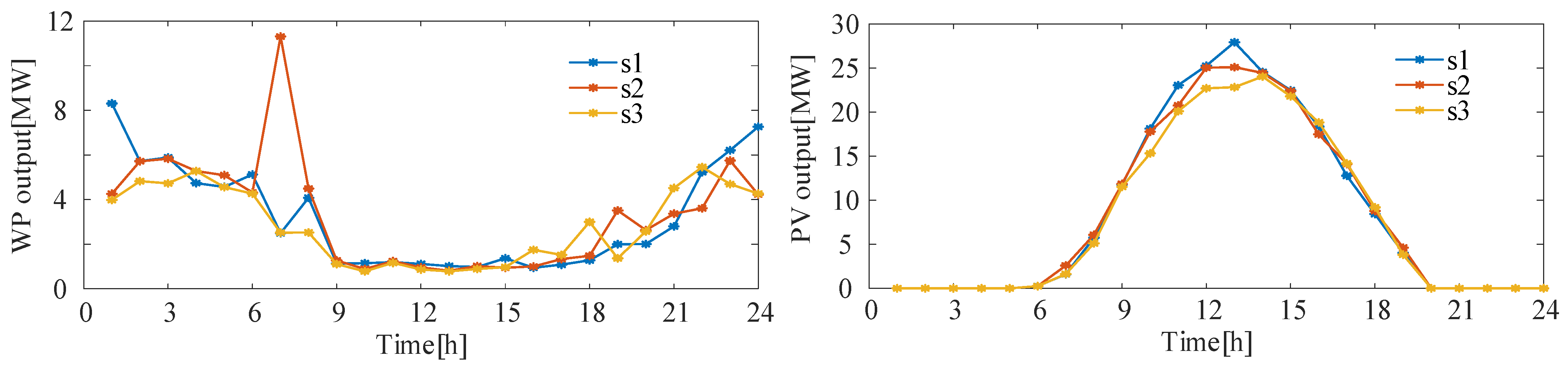
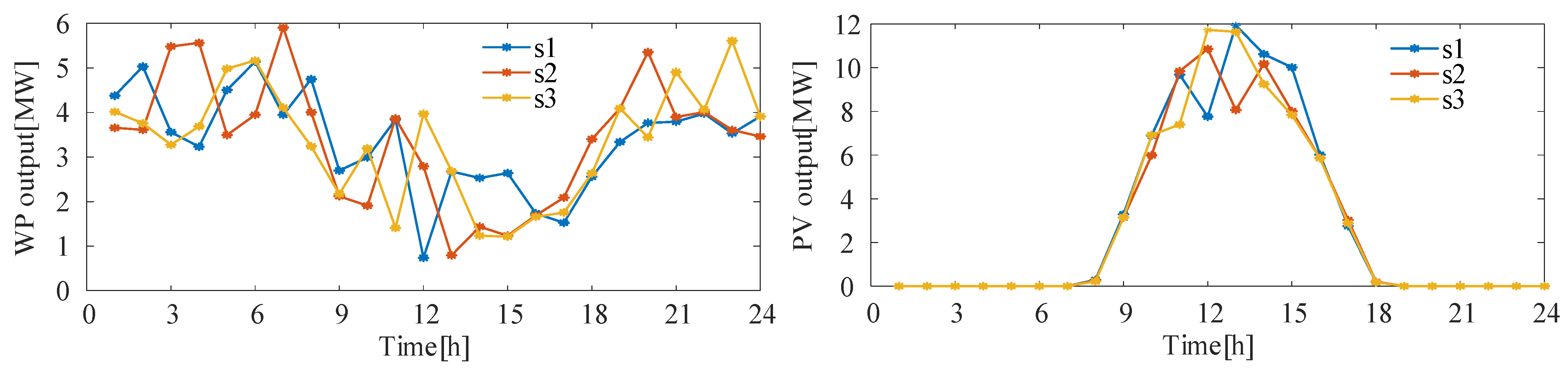
5.2. Generation of Typical Output Scenarios of New Energy

The historical output data of new energy sources were selected from the historical actual measurement data of a WP PV power station in Guangdong, China, from 1 December 2021 to 29 February 2021 and from 1 June 2022 to 31 August 2022. The time scale is 1 h.

Through simulation, we generated three typical wind and PV output scenarios for both summer and winter. The probabilities for summer scenarios (s1, s2, s3) are 0.35467, 0.26667, and 0.37867, respectively, while for winter, they are 0.32933, 0.334, and 0.33667. Figure 3 and Figure 4 present the output data for each scenario in summer and winter, revealing significant seasonal variations in wind and PV power levels, highlighting the need for season-specific planning.

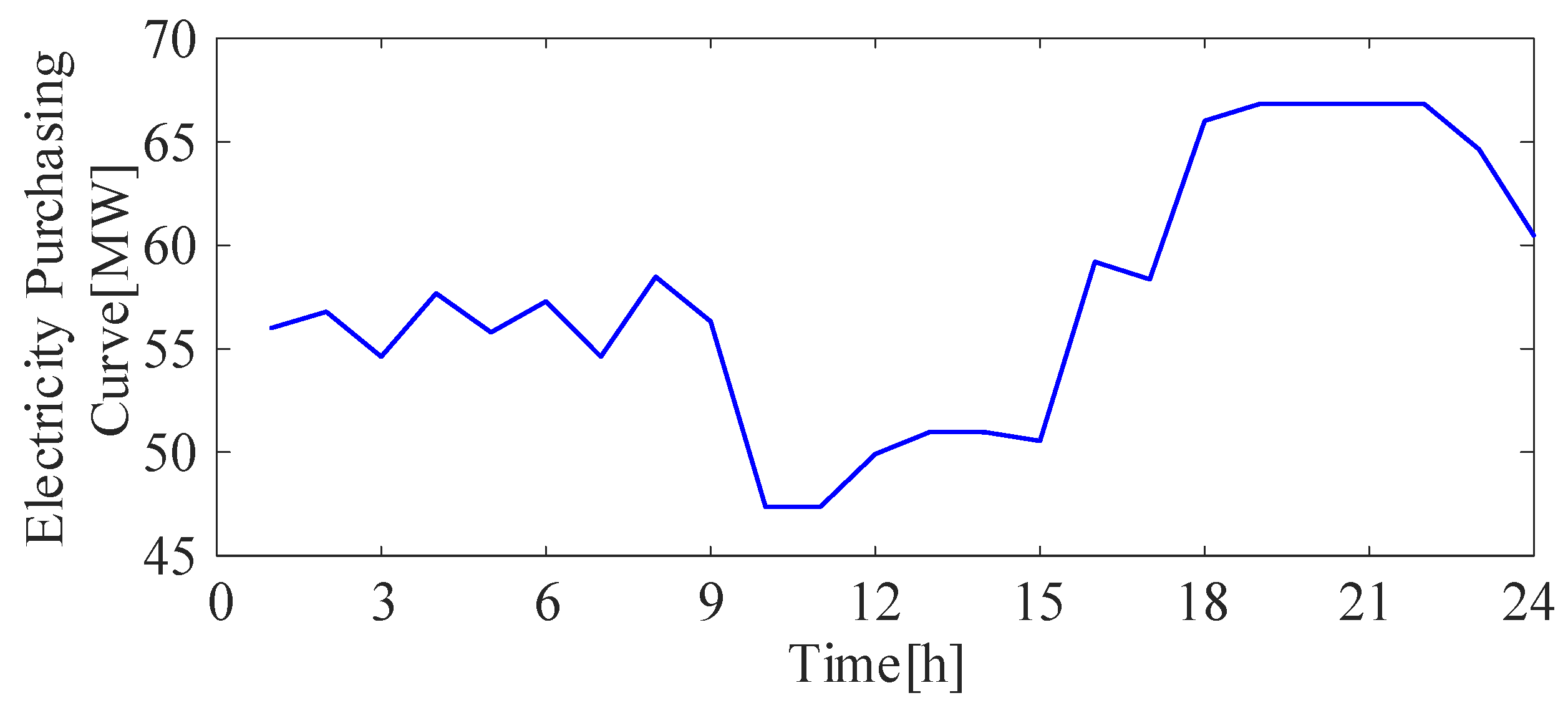
5.3. Planning Results

After solving the problem, the power purchase curve planning decisions for each scenario are consistently illustrated in Figure 5 and Figure 6. The peaking effects for each scenario are compared in Figure 7 and Figure 8. During the off-peak periods (1–5 h and 10–15 h), the system load was low, so electricity purchases were increased to fill the demand valley by boosting refrigerator consumption. Conversely, during the peak periods (6–9 h and 18–22 h), electricity purchases were reduced to lower refrigerator consumption and help shave the peak.

The planning results for each typical scenario are presented in

Table 3. Comparison of the planning results of summer scenarios.

Scenario	Daily Cumulative Power Generation [MW]		FSD Optimization Effect	PVD Optimization Effect	UELD
	WP	PV
1	77.65	204.30	28.78%	35.01%	0.238
2	80.31	201.18	23.35%	28.24%	0.150
3	68.34	191.21	21.49%	25.66%	0.224

and

Table 4. Comparison of the planning results of winter scenarios.

Scenario	Daily Cumulative Power Generation [MW]		FSD Optimization Effect	PVD Optimization Effect	UELD
	WP	PV
1	80.79	69.42	17.06%	34.65%	0.226
2	81.42	65.44	9.71%	34.92%	0.235
3	80.18	67.05	8.97%	19.28%	0.229

. The analysis shows that, due to significant variations in new energy outputs across scenarios, both summer and winter exhibit differing net load fluctuation curves and peak-regulation pressures. Utilizing the SP method proposed in this paper, the resulting daily electricity purchase scheme effectively meets system peak-regulation demands, accounts for user electricity consumption losses, accommodates fluctuating wind and PV outputs, and ensures a comfortable environment in office and cold storage areas. Additionally, it addresses selling pressure indicators.

5.4. Validation of Indicator Nondominations

5.4.1. Validation of the Nondomination of Indicators

In multi-objective optimization, two or more conflicting objective functions are usually involved. In this paper, to find the optimal weight ratio, a fuzzy decision method based on the normalized membership degree value is used in the Pareto solution set. In summer, the target was the minimum level of fluctuation, and the weight of the degree of electricity loss (including the human comfort level of the office area and the hourly average sales pressure of cold storage) was the target. The weight sum of the degree of electricity loss (only including the hourly average sales pressure value of cold storage) is the goal.

The fuzzy membership function is specifically expressed as

$${\psi \left(x\right)}_i^j=\left\{\begin{array}{cc}1,& f_i\le f_i^{\min }\\ {\displaystyle \frac{f_i^{\max }-f_i^j}{f_i^{\max }-f_i^{\min }}},& f_i^{\max }\ge f_i\ge f_i^{\min }\\ 0,& f_i\ge f_i^{\max }\end{array}\right.$$

(26)

where ${\psi \left(x\right)}_i^j$ is the i-th objective function $f_i^j$. The membership function of the j-th solution of $f_i^{max}$ and $f_i^{min}$ represent the maximum and minimum values of the i-th objective function among all nondominated solutions, respectively.

The satisfaction degree of each solution on the Pareto frontal curve is calculated according to the fuzzy membership degree. The solution with the maximum satisfaction value is the optimal plan, and the best compromise solution set is as follows:

$${\eta }_i^{j*}={\max }_{j=1,\cdots ,\mathrm{M}}\left\{{\displaystyle \frac{{\displaystyle \sum _{i=1}^N\psi {(x)}_i^j}}{{\displaystyle \sum _{j=h}^{\mathrm{M}}{\displaystyle \sum _{i=1}^N\psi {(x)}_i^h}}}}\right\}$$

(27)

where M is the number of optimal solutions and N is the number of objective functions.

Regional average values for wind and PV power are determined using historical measured output data from summer and winter, serving as input for WP generation data in the optimization process. Optimal solutions for both summer and winter conditions are derived. For the summer scenario, Figure 9a presents the electricity loss degree index and the Pareto front resulting from the multi-objective joint optimization of payload fluctuation. Similarly, Figure 9b depicts the Pareto front for the multi-objective co-optimization of the electricity consumption degree index and net load fluctuation degree in the winter scenario. This further demonstrates the independence of the load fluctuation index and the UELD index, underscoring the significance of careful planning for both.

5.4.2. Comparison and Validation of the Planning Methods

The average outputs of regional wind and photovoltaic power, calculated from historical measured data, serve as the initial inputs for traditional deterministic optimization. The optimal solution is derived from Section 5.4.1, outlining the peak-shaving potential based on average new energy outputs. Robust optimization, on the other hand, identifies the scenario with the minimum daily accumulated energy from historical data to address output uncertainties and assess its peak-shaving potential.

The comparison results are presented in

Table 5. Comparison of the results of different methods on summer days.

Planning Methods	Proportion of Load Drop During Peak Hour	Proportion of Load Increase During Trough Hours	Daily Electricity Purchase [MW]	UELD
SP	23.87%	22.88%	1380.76	0.209
DO	25.19%	23.63%	1366.94	0.125
RO	10.63%	10.21%	1531.82	0.199

and

Table 6. Comparison of the results of different methods in winter.

Planning Methods	Peak Hour Share Load Reduction Ratio	Share of Trough Time Load Increase Ratio	Daily Electricity Purchase [MW]	UELD
SP	8.08%	8.01%	1029.13	0.167
DO	9.61%	9.68%	1012.94	0.142
RO	5.02%	4.52%	1147.93	0.169

. The analysis reveals that the DO, which uses historical average wind values as input and disregards new energy output time-series fluctuations, yields gentle wind and PV output curves. This reduces peak-regulation pressure on the power system, leading to overly optimistic results with higher peak-regulation potential and lower user electricity loss, thus overestimating the VPP’s peak-regulation capacity. Conversely, the RO method results in lower daily wind and PV outputs, with insufficient new energy output, requiring the system to purchase more grid electricity to meet load demand. The RO method neglects the temporal volatility of renewable energy, thereby avoiding additional aggravation of net load curve fluctuations. This results in a reduced proportion of peak load periods and an increased proportion of valley load periods, ultimately diminishing the adjustability of the load curve. This leads to lower load change proportions and more conservative results that underestimate the system’s peak-regulation potential. Considering Guangdong’s longer summer and shorter winter, the annual peak-regulation potential is calculated via weighted summation, with the summer scenario accounting for two thirds and the winter scenario for one third, as shown in

Table 7. Assessment of annual peak-regulation potential.

Planning Methods	Proportion of Load Drop During Peak Hour	Proportion of Load Increase During Trough Hours
SP	18.61%	17.92%
DO	20.00%	18.98%
RO	8.76%	8.31%

.

Comparative analysis in Figure 10 and Figure 11 shows that both the DO and the RO models yield smoother new energy output and power purchase curves compared to the SP model. In summer, the cooling load comprises office and cold storage area cooling supply, while in winter, it only includes cold storage area cooling supply, resulting in lower cooling load and electricity purchase due to lower ambient temperature. The method presented in this paper considers typical daily operation modes of various new energy units, better simulating wind and PV output time-series fluctuations, thus validating its effectiveness.

5.5. Effect of Temperature-Controlled Flexible Load Change on Peak-Shaving Results

To study the effect of the temperature-controlled flexible load on the peak-regulation performance of the phase system, the summer calculation example is taken as an example, and the following three scenarios are set up for numerical study:

Scenario 1: $\left|I_{PMV}\right|\le 1.2$

Scenario 2: $\left|I_{PMV}\right|\le 1.5$

Scenario 3: $\left|I_{PMV}\right|\le 1.8$

Equation (14) shows that the smaller the absolute value of the PMV index is, the stricter the indoor temperature requirements are, and the more comfortable the human body is. However, the required cooling load is also greater, which also means that the cold energy “storage” capacity of the cooling system is lower. In contrast, the larger the absolute value of the PMV index is, the smaller the cold energy “storage” capacity of the cooling system and the corresponding increase in the response amplitude on the demand side.

The planning results are as shown in

Table 8. Optimization effect comparison table.

Scenario	Comprehensive Optimization Effect
	FSD Optimization Effect	PVD Optimization Effect	UELD
Scenario I	22.74%	26.90%	0.206
Scenario II	24.57%	29.66%	0.209
Scenario III	26.54%	32.41%	0.217

.

The analysis indicates that in Scenario 1, the office area has a narrow allowable PMV fluctuation range, implying low temperature deviation and limited potential for system peak regulation. In Scenario II, the office area operates within a moderate temperature deviation range, offering moderate potential for system peak regulation. In Scenario III, the office area has a higher temperature deviation range, providing greater potential for system peak regulation. Consequently, PSD optimization effects increase by 1.84% and 1.8% across the scenarios, while PVD optimization results rise by 2.74% and 2.75%, respectively. However, user electricity loss increases slightly by 0.011 and 0.013.

6. Conclusions

In this study, a VPP is formed by aggregating WP, PV generation, refrigeration units, and demand response. The uncertainty of new energy output is captured using a scenario-based method, and the objective function optimizes peak regulation while considering user electricity loss. A stochastic planning model for peak regulation in a VPP is established. Using a regional power grid in Guangdong Province as a case study, the following conclusions are drawn:

(1) This paper introduces the UELD, a composite index to measure user losses in VPP DSR. The system is optimized for peak-shaving effectiveness and minimal user loss. Results show that it minimizes user DSR losses while optimizing peak shaving, boosting user participation. VPPs enable integrated optimization of generation and user sides.

(2) To assess the annual peak-regulation potential of the VPP, a simulation method is employed. It evaluates DR potential while considering energy-side generation uncertainty and demand response electricity loss. Optimal flexible load allocation results in a peak-hour load reduction of 18.61% and a trough-hour load reduction of 17.92%.

(3) To tackle new energy output uncertainty, a time-series probabilistic scenario set is used to model wind and PV output variability. This approach reduces optimism compared to deterministic and RO, mitigating conservatism. It aligns more closely with reality in addressing new energy uncertainties and assessing the VPP’s peak-regulation potential.

(4) Limitations and future work: First, approximate processing is applied to multiple parameters in PMV without considering their time-varying characteristics or uncertainties related to extensive user behaviors. Second, approximate processing with subjective experience is adopted for weight coefficients of indicators in the objective function. In addition, current research focuses solely on the peak-shaving-potential analysis of electric-cooling systems. These aspects will be refined and developed in future studies, including the exploration of multi-energy systems and multi-energy VPPs possibilities.

References

1. Zhang, S.; Pan, G.; Li, B.; Gu, W.; Fu, J.; Sun, Y. Multi-Timescale Security Evaluation and Regulation of Integrated Electricity and Heating System. IEEE Trans. Smart Grid 2025, 16, 1088–1099. [Google Scholar] [CrossRef]
2. Qiu, W.; Yin, H.; Dong, Y.; Wei, X.; Liu, Y.; Yao, W. Synchro-Waveform-Based Event Identification Using Multi-Task Time-Frequency Transform Networks. IEEE Trans. Smart Grid 2025, 16, 2647–2658. [Google Scholar] [CrossRef]
3. Arteconi, A.; Polonara, F. Assessing the Demand Side Management Potential and the Energy Flexibility of Heat Pumps in Buildings. Energies 2018, 11, 1846. [Google Scholar] [CrossRef]
4. Navesi, R.B.; Naghibi, A.F.; Zafarani, H.; Tahami, H.; Pirouzi, S. Reliable operation of reconfigurable smart distribution network with real-time pricing-based demand response. Electr. Power Syst. Res. 2025, 241, 111341. [Google Scholar] [CrossRef]
5. Vanhoudt, D.; Geysen, D.; Claessens, B.; Leemans, F.; Jespers, L.; Van Bael, J. An actively controlled residential heat pump: Potential on peak shaving and maximization of self-consumption of renewable energy. Renew. Energy 2014, 63, 531–543. [Google Scholar] [CrossRef]
6. Sæther, G.; Granado, P.C.D.; Zaferanlouei, S. Peer-to-peer electricity trading in an industrial site: Value of buildings flexibility on peak load reduction. Energy Build. 2021, 236, 110737. [Google Scholar] [CrossRef]
7. Zheng, M.; Meinrenken, C.J.; Lackner, K.S. Agent-based model for electricity consumption and storage to evaluate economic viability of tariff arbitrage for residential sector demand response. Appl. Energy 2014, 126, 297–306. [Google Scholar] [CrossRef]
8. Liu, Z.; Zhu, R.; Kong, D.; Guo, H. Coordinated Operation Strategy for Equitable Aggregation in Virtual Power Plant Clusters with Electric Heat Demand Response Considered. Energies 2024, 17, 2640. [Google Scholar] [CrossRef]
9. Dong, Z.; Zhang, Z.; Huang, M.; Yang, S.; Zhu, J.; Zhang, M.; Chen, D. Research on day-ahead optimal dispatching of virtual power plants considering the coordinated operation of diverse flexible loads and new energy. Energy 2024, 297, 131235. [Google Scholar] [CrossRef]
10. Luo, Z.; Hong, S.; Ding, Y. A data mining-driven incentive-based demand response scheme for a virtual power plant. Appl. Energy 2019, 239, 549–559. [Google Scholar] [CrossRef]
11. Li, D.; Wang, M.; Shen, Y.; Li, F.; Lin, S.; Zhou, B. Low-carbon operation strategy of virtual power plant considering progressive demand response. Int. J. Electr. Power Energy Syst. 2024, 161, 110176. [Google Scholar] [CrossRef]
12. Su, S.; Hu, G.; Li, X.; Li, X.; Xiong, W. Electricity-Carbon Interactive Optimal Dispatch of Multi-Virtual Power Plant Considering Integrated Demand Response. Energy Eng. 2023, 120, 2343–2368. [Google Scholar] [CrossRef]
13. Mei, S.; Tan, Q.; Liu, Y.; Trivedi, A.; Srinivasan, D. Optimal bidding strategy for virtual power plant participating in combined electricity and ancillary services market considering dynamic demand response price and integrated consumption satisfaction. Energy 2023, 284, 128592. [Google Scholar] [CrossRef]
14. Wang, Y.; Yang, Y.; Tang, L.; Sun, W.; Li, B. A Wasserstein based two-stage distributionally robust optimization model for optimal operation of CCHP micro-grid under uncertainties. Int. J. Electr. Power Energy Syst. 2020, 119, 105941. [Google Scholar] [CrossRef]
15. Parvar, S.S.; Nazaripouya, H. Optimal Operation of Battery Energy Storage Under Uncertainty Using Data-Driven Distributionally Robust Optimization. Electr. Power Syst. Res. 2022, 211, 108180. [Google Scholar] [CrossRef]
16. Aghdam, F.H.; Javadi, M.S.; Catalão, J.P.S. Optimal stochastic operation of technical virtual power plants in reconfigurable distribution networks considering contingencies. Int. J. Electr. Power Energy Syst. 2023, 147, 108799. [Google Scholar] [CrossRef]
17. Wang, J.; Lei, T.; Qi, X.; Zhao, L.; Liu, Z. Chance-constrained optimization of distributed power and heat storage in integrated energy networks. J. Energy Storage 2022, 55, 105662. [Google Scholar] [CrossRef]
18. Kazemtarghi, A.; Mallik, A. A two-stage stochastic programming approach for electric energy procurement of EV charging station integrated with BESS and PV. Electr. Power Syst. Res. 2024, 232, 110411. [Google Scholar] [CrossRef]
19. Al-Lawati, R.A.H.; Faiz, T.I.; Noor-E-Alam, M. A nationwide multi-location multi-resource stochastic programming based energy planning framework. Energy 2024, 295, 130898. [Google Scholar] [CrossRef]
20. Ebeed, M.; Alhejji, A.; Kamel, S.; Jurado, F. Solving the Optimal Reactive Power Dispatch Using Marine Predators Algorithm Considering the Uncertainties in Load and Wind-Solar Generation Systems. Energies 2020, 13, 4316. [Google Scholar] [CrossRef]
21. Lin, S.; Liu, C.; Shen, Y.; Li, F.; Li, D.; Fu, Y. Stochastic Planning of Integrated Energy System via Frank-Copula Function and Scenario Reduction. IEEE Trans. Smart Grid 2022, 13, 202–212. [Google Scholar] [CrossRef]
22. Wan, Q.; Yu, Y. Power load pattern recognition algorithm based on characteristic index dimension reduction and improved entropy weight method. Energy Rep. 2020, 6, 797–806. [Google Scholar] [CrossRef]
23. Ismkhan, H. I-k-means−+: An iterative clustering algorithm based on an enhanced version of the k-means. Pattern Recognit. 2018, 79, 402–413. [Google Scholar] [CrossRef]
24. Onumanyi, A.J.; Molokomme, D.N.; Isaac, S.J.; Abu-Mahfouz, A.M. AutoElbow: An Automatic Elbow Detection Method for Estimating the Number of Clusters in a Dataset. Appl. Sci. 2022, 12, 7515. [Google Scholar] [CrossRef]
25. Duan, C.; Ding, X.; Shi, F.; Xiao, X.; Duan, P. PMV-based fuzzy algorithms for controlling indoor temperature. In Proceedings of the 2011 6th IEEE Conference on Industrial Electronics and Applications, Beijing, China, 21–23 June 2011; pp. 1492–1496. [Google Scholar]
26. Donaisky, E.; Oliveira, G.H.C.; Freire, R.Z.; Mendes, N. PMV-Based Predictive Algorithms for Controlling Thermal Comfort in Building Plants. In Proceedings of the 2007 IEEE International Conference on Control Applications, Singapore, 1–3 October 2007; pp. 182–187. [Google Scholar]
27. Gormley, R.; Walshe, T.; Hussey, K.; Butler, F. The Effect of Fluctuating vs. Constant Frozen Storage Temperature Regimes on Some Quality Parameters of Selected Food Products. LWT—Food Sci. Technol. 2002, 35, 190–200. [Google Scholar] [CrossRef]
28. Zhou, J.; Zhang, J.; Qiu, Z.; Yu, Z.; Cui, Q.; Tong, X. Two-Stage Robust Optimization for Large Logistics Parks to Participate in Grid Peak Shaving. Symmetry 2024, 16, 949. [Google Scholar] [CrossRef]
29. Li, Z.; Sun, Z.; Meng, Q.; Wang, Y.; Li, Y. Reinforcement learning of room temperature set-point of thermal storage air-conditioning system with demand response. Energy Build. 2022, 259, 111903. [Google Scholar] [CrossRef]
Figure 1. Basic structure of a VPP.
Symmetry 17 00683 g001
Figure 2. General flow chart.
Symmetry 17 00683 g002
Figure 3. Summer scenery contribution scene collection.
Symmetry 17 00683 g003
Figure 4. A collection of winter scenery output scenes.
Symmetry 17 00683 g004
Figure 5. Summer electricity purchase curve planning results.
Symmetry 17 00683 g005
Figure 6. Winter power purchase curve planning results of winter.
Symmetry 17 00683 g006
Figure 7. Comparison diagram of peak-shaving effects in summer scenarios.
Symmetry 17 00683 g007
Figure 8. Comparison diagram of peak-shaving effects in winter scenarios.
Symmetry 17 00683 g008
Figure 9. Pareto boundary.
Symmetry 17 00683 g009
Figure 10. Day-ahead power purchase curve planning results via different methods in the summer scenario.
Symmetry 17 00683 g010
Figure 11. Day-ahead power purchase curve planning results via different methods in the winter scenario.
Symmetry 17 00683 g011