A Cooperative MHE-Based Distributed Model Predictive Control for Voltage Regulation of Low-Voltage Distribution Networks

Abstract

This paper presents a moving horizon estimator-based cooperative model predictive control strategy for a low-voltage distribution area equipped with symmetric distributed generators (DGs). First, DGs have their symmetries in the control structures that can be utilized for the control design. Then, a simplified model using feedback linearization theory for the symmetric DGs with hierarchical control reduces the high-order detailed models to low-order ones. To supplement the loss of accuracy and reliability in the proposed model, the controller introduces a moving horizon estimator to observe the unmeasured state variables under the poor communication condition of a low-voltage distribution network. Compared to the conventional method, the moving horizon estimator has advantages in handling uncertain disturbances, communication delays, constraints, etc. Furthermore, with all measured and observed state information, a cooperative distributed model predictive controller can be executed, and the stability and feasibility of controller are given. Finally, the effectiveness of the proposed control technique is verified through simulation based on Matlab/Simulink.

1. Introduction

The increasing penetration of distributed generators (DGs) in modern distribution systems has transformed conventional passive grids into active power networks with integrated generation, storage, and load management capabilities [1,2,3]. While this transition enhances energy efficiency and sustainability, it introduces new technical challenges such as power quality degradation, voltage instability, and bidirectional power flow dynamics. Particularly in low-voltage distribution networks (LVDNs) characterized by limited communication infrastructure and complex topologies, the stochastic nature of DGs exacerbates voltage regulation issues [4,5].

Over the past decades, significant research efforts have focused on voltage management strategies, leveraging the operational flexibility of symmetrical renewable energy resources in distribution systems [6,7]. These approaches exploit control redundancies in symmetrical DG inner loops to enhance grid resilience. However, implementing dynamic voltage regulation in LVDNs remains challenging due to some critical technical barriers. Firstly, compared with the conventional automatic voltage control system, the communication structure in the low-voltage distribution area is incomplete. The centralized controller is hard to manage all the DGs with symmetries [8]. Secondly, conventional wireless communication is the main channel to connect the adjacent DGs, and communication delay is inevitable in this scene [9,10]. Thirdly, the unclear topology and line parameters in these areas cause issues in modeling the overall system [11,12,13]. Therefore, traditional voltage control technology based on the voltage sensitivity model cannot be applied appropriately in this scenario. Consequently, there is an urgent need to construct a stable and dynamic voltage control system for multiple symmetrical resources to improve the voltage regulation in the LVDN.

Researchers have devoted significant efforts to voltage regulation in distribution networks using centralized automatic voltage control systems [14,15], which serve as the foundation for initiating control actions. Existing studies on voltage control predominantly focus on static optimization objectives, such as power flow optimization and voltage deviation minimization [16,17,18]. However, in LVDNs, particularly demand-side networks, strict adherence to static optimality may be unnecessary, as these systems primarily aim to meet upstream grid demands. Instead, dynamic voltage security and stability are critical for ensuring reliable power delivery to low-voltage consumers [19,20,21], where the inherent control symmetries of DGs can be strategically leveraged.

A key challenge in LVDNs is the lack of robust communication infrastructure compared to high-voltage distribution networks. This necessitates the adoption of distributed control architectures for symmetrical DGs, though communication delays inevitably arise during dynamic voltage regulation [22]. Such delays introduce time asynchronization in control signals, degrading system performance and potentially destabilizing the network [23]. Recent work addresses this issue through predictive control strategies. For example, reference [24] proposes a distributed cooperative control framework for cyber-physical microgrids with communication delays, enabling DG voltage restoration. Similarly, reference [25] compares a Smith-predictor-based and an MPC-based method for delay compensation in secondary control, demonstrating MPC’s superior robustness. However, existing studies primarily focus on compensating for communication delays and overlook adaptation to internal controller-induced delays.

As a mature control technology, MPC has been deeply studied during the past decades and applied in optimization and dynamic control. The MPC has been widely used in the power flow optimization of distribution networks [26,27,28,29], which maximizes the operation effect of the distribution grid in one static operation. As in voltage source converters [30,31], the MPC-based controllers can help converters to improve their dynamic performances and promote the stability and robustness of the utility grid. In the current active LVDN, MPC is still seldom exploited and needs to be improved to serve dynamic voltage control.

To address the deficiencies, we proposed a cooperative MHE-based distributed model predictive control to serve the voltage control in LVDNs. The main contributions are listed as follows:

• A distributed control scheme is implemented in the low-voltage distribution network (LVDN) without relying on the system structure and topology information. This approach effectively exploits the symmetries of distributed generators. Given the challenging communication conditions and complex, often ill-defined structures in LVDNs, this utilization of DG symmetries is of great significance. Compared with traditional methods that demand comprehensive system information, the proposed distributed control scheme offers a more practical and adaptable solution for LVDN control;
• The feedback linearization theory is employed to simplify the high-order and nonlinear DG model. Through this approach, the order of the model is reduced, and the input–output relationship is decoupled. This simplification greatly facilitates the design of the secondary controller. In the context of voltage control in LVDNs, the application of feedback linearization provides a more efficient means of handling the complex DG model, enhancing the manageability of the control system design process;
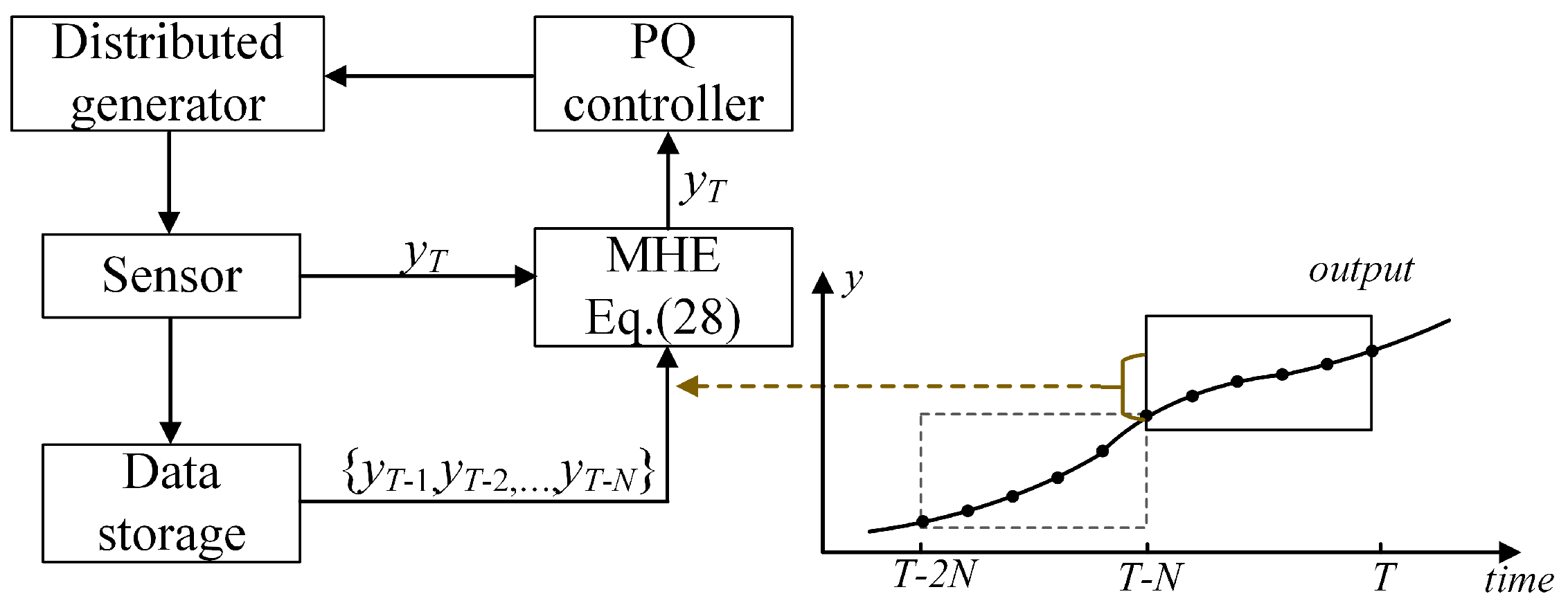
• A moving horizon estimator is proposed to estimate the internal deficient state variables. By estimating these variables, the dynamic response of voltage control is improved, and the measurement limitations in low-voltage distribution networks are compensated. In particular, after the feedback linearization reduces the model order, some state variables may become unmeasurable. MHE effectively addresses this issue. It can handle the nonlinear characteristics of the model, thereby enhancing the accuracy and reliability of state variable estimation. This represents a significant advancement over traditional estimation methods, contributing to more effective voltage control in LVDNs;
• Considering the inevitable time delay in the communication link, a cooperative moving horizon estimator-based distributed model predictive control (MPC) is proposed. This control method enhances the coordination among different DGs and improves the robustness of the low-voltage distribution network. In the secondary control, it adjusts the control signal to account for the time delay, thereby improving the performance of conventional control methods under poor communication conditions. The proposed cooperative MHE-based distributed MPC provides a more reliable and efficient control strategy for LVDNs in the face of communication challenges.

The rest of this paper is organized as follows. The basic operating condition of the LVDN is presented in Section 2. Section 3 gives the basic primary and secondary control method. In Section 4, a cooperative MHE-based distributed MPC is presented. In Section 5, simulation results and discussions are shown. Finally, the paper is concluded in Section 6.

2. Grid-Connected Low-Voltage Distribution Network

2.1. Distributed Structure

Distributed structure needs to decompose the overall system model of the distribution network into relative subsystem models. A system comprised of interconnected subsystems is used to illustrate these concepts.

The centralized overall system state space model is usually expressed as a discrete linear time-invariant model in the following form:

$$\left\{\begin{array}{c}x(k+1)=Ax\left(k\right)+Bu\left(k\right)\hfill \\ y\left(k\right)=Cx\left(k\right)\hfill \end{array}\right.$$

(1)

where k denotes discrete time; u, x, and y, respectively, denote the system input, state, and output vector; and $A,B,C$ are, respectively, system, control, and output matrices, as follows:

$$A=\left[\begin{array}{ccc}{A}_{11}& \dots & A_{N1}\\ ⋮& \ddots & ⋮\\ A_{N1}& \dots & A_{NN}\end{array}\right],B=\left[\begin{array}{ccc}{B}_{11}& \dots & B_{N1}\\ ⋮& \ddots & ⋮\\ B_{N1}& \dots & B_{NN}\end{array}\right]$$

$$C=\left[\begin{array}{ccc}{C}_{11}& \dots & 0\\ ⋮& \ddots & ⋮\\ 0& \dots & C_{NN}\end{array}\right]$$

(2)

In the distributed structure, the subsystem model contains the local subsystem variable and the effect of interconnected subsystems. Therefore, the overall model in (1) can be rewritten as the following form:

$$\left\{\begin{array}{c}{x}_i(k+1)=A_{ii}{x}_i\left(k\right)+B_{ii}{u}_i\left(k\right)+{\displaystyle \sum _{j\ne i}^N}{A}_{ij}{x}_j\left(k\right)\hfill \\ y_i\left(k\right)=C_{ii}x\left(k\right)\hfill \end{array}\right.$$

(3)

where $x_i,u_i,y_i$ denote the state, control, and output variable of the distributed system model in (3), and $A_{ii},A_{ij}$ are, respectively, the system matrix of subsystem i and interaction matrix between subsystems i and j.

2.2. Communication Delay

In the LVDN, it is unnecessary and impractical to establish an optical fiber communication network as the medium-voltage distribution network. Thus, the time delay is a non-negligible issue in the LVDN voltage control. According to Equation (3), the time-delay state-space model can be transformed into

$$\left\{\begin{array}{c}{x}_i(k+1)=A_{ii}{x}_i\left(k\right)+B_{ii}{u}_i\left(k\right)+{\displaystyle \sum _{j\ne i}^N}{A}_{ij}{x}_j(k-\tau )\hfill \\ y_i\left(k\right)=C_{ii}x\left(k\right)\hfill \end{array}\right.$$

(4)

where $\tau >0$ is a constant denoting the communication time delay of the state variable, assuming $0\le \tau \le {\tau }^{*}$ with a bounded value of ${\tau }^{*}$.

For distributed generators, the time for local control is approximately a few milliseconds. Therefore, compared to the interaction delay, the local time delay is ignored in Model (4).

2.3. Voltage Sensitivity with Respect to Power Injection

In this paper, a low-voltage distribution area is assumed to include $N+1$ buses represented by $0,1,2,\dots ,N$. Bus 0 denotes the slack bus, which is connected to the higher-level electricity grid through a substation transformer. For other buses, the relationship between injection power (active power $\Delta P$ and reactive power $\Delta Q$) and bus voltage (phase $\Delta \theta$ and amplitude $\Delta V$) can be obtained according to the conventional power flow equations, which can be transferred as follows [32,33,34]:

$$\left[\begin{array}{c}\Delta P\left(t\right)\\ \Delta Q\left(t\right)\end{array}\right]=\left[\begin{array}{cc}{J}_1& J_2\\ J_3& J_4\end{array}\right]\left[\begin{array}{c}\Delta \theta \left(t\right)\\ \Delta V\left(t\right)\end{array}\right]$$

(5)

where $\Delta P\left(t\right)={[\Delta P_1,\Delta P_2,\cdots ,\Delta P_N]}^T$, $\Delta Q\left(t\right)={[\Delta Q_1,\Delta Q_2,\cdots ,\Delta Q_N]}^T$, $\Delta V\left(t\right)={[\Delta V_1,\Delta V_2,\cdots ,\Delta V_N]}^T$, $\Delta \theta \left(t\right)={[\Delta {\theta }_1,\Delta {\theta }_2,\cdots ,\Delta {\theta }_N]}^T$. The elements of matrix $J_1$,$J_2$,$J_3$,$J_4$ are as below:

$$J_{1,ij}=\left[{\displaystyle \frac{\partial P_i}{\partial {\theta }_j}}\right],J_{2,ij}=\left[{\displaystyle \frac{\partial P_i}{\partial V_j}}\right],J_{3,ij}=\left[{\displaystyle \frac{\partial Q_i}{\partial {\theta }_j}}\right],J_{4,ij}=\left[{\displaystyle \frac{\partial Q_i}{\partial V_j}}\right].$$

$J_1$ is assumed to be invertible; then, the voltage sensitivity can be represented, from (5), as

$$\begin{array}{cc}\hfill \Delta V\left(t\right)& ={(J_4-J_3{J}_1^{-1})}^{-1}[\Delta Q\left(t\right)-J_3{J}_1^{-1}\Delta P\left(t\right)]\hfill \\ \hfill & =S_{VQ}\Delta Q\left(t\right)+S_{VP}\Delta P\left(t\right)\hfill \end{array}$$

(6)

where $S_{VQ}$ and $S_{VP}$ are the voltage sensitivity matrix with respect to active and reactive injected power, and $S_{VQ}={(J_4-J_3{J}_1^{-1})}^{-1}$, $S_{VP}=-{(J_4-J_3{J}_1^{-1})}^{-1}{J}_3{J}_1^{-1}$.

The $S_{VQ}$ and $S_{VP}$ are time-variant according to the different operating conditions of LVDN. Equation (5) gives a commonly used linearized form at any working condition of distribution networks.

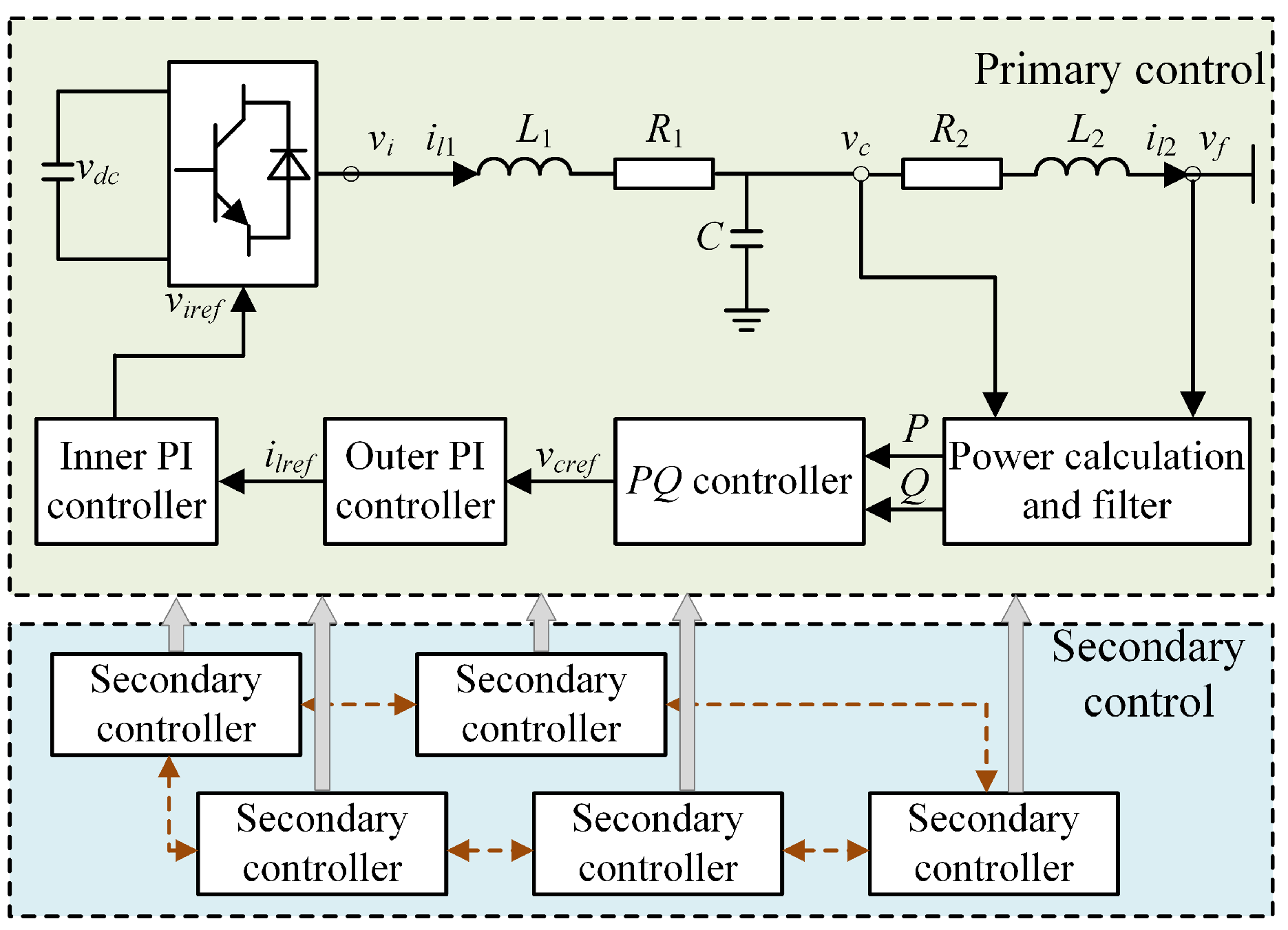
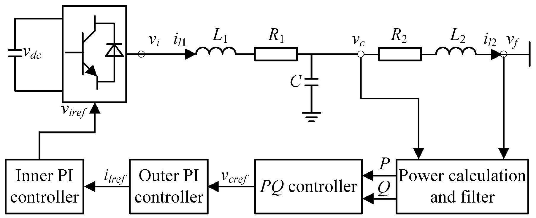
3. Control System of Distributed Generators

3.1. Power and Current Control Systems

To improve the voltage control capacity of the LVDC, DGs typically employ a hierarchical control structure to coordinate strategies across different time scales. This paper focuses on dynamic voltage control techniques, which encompass primary and secondary control mechanisms. Dynamic control means providing second control for processing voltage events, and the long-timescale economic optimization is not discussed in this paper. The overall control scheme is shown in Figure 1. The primary control layer utilizes a PQ strategy, and the secondary control layer implements a distributed control architecture.

3.2. Primary Control with Symmetries

The LVDN in this paper is connected to the upper power grid. Thus, the electric converters of DGs adopt a grid-following control strategy. The scheme of grid-connected DG is shown in Figure 2, which contains many symmetrical parts. Each control loop adopts the dq-axis symmetrical control as follows. The detailed model of DG in this paper can be described as follows.

The model of phase is represented as

$$\dot{\delta }=\omega -{\omega }_{ref}$$

(7)

where $\omega$ and ${\omega }_{ref}$, respectively, denote the practical and referential angular velocity of DG; $\delta$ is the angle of DG.

The model of symmetrical power outputs can be established as

$$\left\{\begin{array}{c}{P}_o={\displaystyle \frac{{\omega }_c}{s+{\omega }_c}}(v_{cd}{i}_{l1d}+v_{cq}{i}_{l1q})\hfill \\ Q_o={\displaystyle \frac{{\omega }_c}{s+{\omega }_c}}(v_{cd}{i}_{l1q}-v_{cq}{i}_{l1d})\hfill \end{array}\right.$$

(8)

where ${\omega }_c$ is the cutoff frequency of the low-pass filter; $P_o$ and $Q_o$ are the output active and reactive power of DG; and $v_{cd}$, $v_{cq}$, $i_{l1d}$, $i_{l1q}$ are the $dq$ component of DG’s filter capacitor (C) voltages and $dq$ component of DG’s currents flowing in the filter inductance $L_1$. The detailed relationship between each variable can be seen in Appendix A.

3.3. Secondary Control

The primary PQ control of DG can realize a rapid track of power reference for a higher level of the distribution network. The secondary control layer needs to compute suitable instructions to control the bus voltage to converge on a safe section (0.95 p.u.–1.05 p.u.). To suppress the voltage deviation, PI control is introduced to implement the secondary control. The control signal can be generated as follows:

$$u_{i,sec}=\sum _{j=1}^{N_s}{\alpha }_{ij}\Delta v_j({\displaystyle \frac{k_{I,ij}}{s}}+k_{P,ij})$$

(9)

where $u_{i,sec}$ denotes the secondary control signal of the $i^{th}$ DG; ${\alpha }_{ij}$ is the adjustment coefficient of the $i^{th}$ DG; $\Delta v_j$ represents the voltage deviation of bus connected to the $j^{th}$ DG; $k_{P,ij}$ and $k_{I,ij}$ are, respectively, the secondary proportion and integral coefficient of the $j^{th}$ DG; and $N_i$ is the number of DGs connected to the $i^{th}$ DG.

In distributed control structure, if the $i^{th}$ and $j^{th}$ DG can exchange information with each other, ${\alpha }_{ij}$ = 1; else, ${\alpha }_{ij}$ = 0. $k_{P,ij}$ and $k_{I,ij}$ are decided by the voltage sensitivity matrices $S_{VQ}$ and $S_{VP}$.

Considering the poor communication conditions of low-voltage distribution areas, the DG cannot receive the adjacent state information immediately. The time delay will lead to the asynchronization of control signals, which may cause the instability of the system. Therefore, we transform Equation (9) into the following form with a time delay:

$$\begin{array}{cc}\hfill u_{i,sec}& ={\alpha }_{ii}\Delta v_i\left(k\right)({\displaystyle \frac{k_{I,ii}}{s}}+k_{P,ii})\hfill \\ & +\sum _{j=1,j\ne i}^N{\alpha }_{ij}\Delta v_j(k-\tau )({\displaystyle \frac{k_{I,ij}}{s}}+k_{P,ij})\hfill \end{array}$$

(10)

where k denotes the sample time and $\tau$ denotes the time delay.

4. Prediction-Based Secondary Control for Voltage Regulation

4.1. Feedback Linearization Theory

Considering that the model of DG is nonlinear and of a high order, it is difficult to design the control with this detailed model. Therefore, a feedback linearization theory is introduced to reduce the order of the DG model and decouple the relationship between the input and output variables of DG. A more involved explanation on theory and study of feedback linearization can be found in [35,36].

According to Equations (7)–(10), a multi-input and multi-output (MIMO) system is established as follows:

$$\begin{array}{c}\dot{x}=f\left(x\right)+g\left(x\right)u\hfill \end{array}$$

(11)

$$y=h\left(x\right)$$

(12)

where x and u are, respectively, the n and m row vector. x = ${[\omega ,P,Q,i_d,i_q,v_d,v_q,i_{l1d},i_{l1q},v_{cd},v_{cq},v_{id},v_{iq},i_{l2d},i_{l2q}]}^T$, u = ${[P_{ref},Q_{ref},v_{fd},v_{fq}]}^T$; y = ${[P,Q,v_{cd},v_{cq}]}^T$; $f\left(x\right),g\left(x\right)$ denote functions of the system model.

Lemma 1.

Suppose that the matrix $g\left(x_o\right)$ has rank m, where $x_0$ is the initial state. Then, the linearization problem of state space is solvable if and only if there exist a neighborhood U of $x_o$ and m real-valued functions $h_1\left(x\right)$, $h_2\left(x\right)$, …, $h_m\left(x\right)$ defined on U that have some (vector) relative degree $r_1,r_2,\dots ,r_m$ at $x_o$ and $r_1+r_2+\dots +r_m=n$.

According to feedback linearization theory, the output y will be differentiated until at least one input variable $u_i$ appears. In this paper, $L_{f}h\left(x\right)$ and $L_{g}h\left(x\right)$ are, respectively, defined as $Lie$ derivatives of $h\left(x\right)$ along f and g, where

$$\left\{\begin{array}{c}\hfill L_{f}h\left(x\right)={\displaystyle \frac{\partial h}{\partial x}}f\left(x\right)\\ \hfill L_{g}h\left(x\right)={\displaystyle \frac{\partial h}{\partial x}}g\left(x\right)\end{array}\right.$$

(13)

Therefore, Equation (12) can be transferred as follows:

$${\dot{y}}_i=L_f{h}_i\left(x\right)+\sum _{j=1}^m\left(L_{g_i}{h}_j\left(x\right)\right)u_j$$

(14)

In this case, if the following equation is satisfied,

$$\left\{\begin{array}{c}{L}_{g}h\left(x\right)=L_g{L}_{f}h\left(x\right)=\cdots =L_g{L}_f^{r_m-2}h\left(x\right)=0\hfill \\ L_g{L}_f^{r_m-1}h\left(x\right)={\displaystyle \frac{\partial L_f^{r_m-1}h}{\partial x}}g\left(x\right)\ne 0\hfill \end{array}\right.$$

(15)

then the input appears after $r_m$ deviations of (14) as follows:

$$y_i^{\left(r_m\right)}=L_f^{\left(r_m\right)}{h}_i\left(x\right)+\underset{m}{\sum ^{j=1}}{L}_{g_j}{L}_f^{\left(r_m-1\right)}{h}_i\left(x\right)u_j$$

(16)

where $i=1,2,\dots ,m$. Equation (16) can be described in a matrix form as

$$\left[\begin{array}{c}{y}_1^{\left(r_1\right)}\\ ⋮\\ y_m^{\left(r_m\right)}\end{array}\right]=\left[\begin{array}{c}{L}_f^{\left(r_1\right)}{h}_1\left(x\right)\\ ⋮\\ L_f^{\left(r_m\right)}{h}_m\left(x\right)\end{array}\right]+F\left(x\right)\left[\begin{array}{c}{u}_1\\ ⋮\\ u_m\end{array}\right]$$

(17)

where

$$F\left(x\right)=\left[\begin{array}{ccc}{L}_{g_1}{L}_f^{r_1-1}{h}_1\left(x\right)& \cdots & L_{g_{m1}}{L}_f^{r_1-1}{h}_1\left(x\right)\\ L_{g_1}{L}_f^{r_2-1}{h}_2\left(x\right)& \cdots & L_{g_{m_1}}{L}_f^{r_2-1}{h}_2\left(x\right)\\ \cdots & \cdots & \cdots \\ L_{g_1}{L}_f^{r_{1m}-1}{h}_m\left(x\right)& \cdots & L_{g_m}{L}_f^{r_m-1}{h}_{m_l}\left(x\right)\end{array}\right]$$

Assumption 1.

For a system of the form in (11): (i) $L_{gi}{L}_f^k{h}_i\left(x\right)=0$, for all $1\le j\le m$, for $1\le i\le m$, and for all x in a neighborhood of $x_0$; ($ii$) the $m\times m$ matrix $F\left(x\right)$ is nonsingular at $x=x_o$.

According to [36], satisfying Lemma 1 and Assumption 1, a solution can be found for choices of output functions $h_i\left(x\right)$. The input can be transformed as

$$u=-F^{-1}\left(x\right)\left[\begin{array}{c}{L}_f^{\left(r_1\right)}{h}_1\left(x\right)\\ ⋮\\ L_f^{\left(r_m\right)}{h}_m\left(x\right)\end{array}\right]+F^{-1}\left(x\right)\left[\begin{array}{c}{v}_1\\ ⋮\\ v_m\end{array}\right]$$

(18)

where $v={[v_1,\dots ,v_m]}^T$ is the new input of designed system with feedback linearization.

4.2. Moving Horizon Estimation

The high-order DG model is simplified to a low-order one with feedback linearization, but there are still some unmeasurable variables in the reduced-order model. Moreover, intermediate variables $L_{gj}{L}_f^k{h}_i\left(x\right)$ contain many state variables. To obtain these state variables, sensors need to be set up, which increases the application cost of DGs. These issues can have a negative impact on the control of DGs. Therefore, moving horizon estimation (MHE) is introduced in this section to obtain unmeasurable variables for better characteristics of the DG system and minimize the influence of measurement noise. The principle of MHE is shown in Figure 3. MHE uses a model to forecast a system’s behavior over a certain horizon based on an initial estimate of the system’s state (prior) [37]. Since the prior is usually inaccurate, it is important to adjust it to generate a state trajectory that better aligns with the measurements. MHE can handle the nonlinear characteristics of the model and improve the accuracy and reliability of estimated state variables with constraints of additional information about DGs. It does not require all the dynamic data during the control process and is compatible with the model obtained by the feedback linearization method.

In this paper, the value of m is taken as four; then, we can obtain a common state-space model based on Equation (17) and the linearization method [37] as follows:

$$\left\{\begin{array}{c}{\dot{x}}_{DG}=A_{DG}{x}_{DG}+B_{DG}{v}_{DG}\hfill \\ y_{DG}=C_{DG}{x}_{DG}\hfill \end{array}\right.$$

(19)

where $x_{DGi}={[x_1,x_2,x_3,x_4,x_5,x_6]}^T$, $x_1=P$, $x_2=Q$, $x_3=v_{l1d}$, $x_4=v_{l1q}$, $x_5=v_{l2d}$, $x_6={\dot{v}}_{l2q}$; $y_{DGi}={[x_1,x_2,x_3,x_4]}^T$; $A_{DG}$ and $B_{DG}$ are the relevant system and control matrix; and $C_{DG}$ is the output matrix.

In the MPC structure, multiple measured data can be used to estimate the states of the system. The M sets of closest measured output data are before time T are recorded as follows:

$${\left\{y_{DG,i}\right\}}_{T-M}^{T-1}:=\left\{y_{DG,T-M},y_{DG,T-M+1},\cdots ,y_{DG,T-1}\right\}$$

(20)

The M sets of closest measured disturbance data before time T are recorded as follows:

$${\left\{v_{DG,i}\right\}}_{T-M}^{T-1}:=\left\{v_{DG,T-M},v_{DG,T-M+1},\cdots ,v_{DG,T-1}\right\}$$

(21)

Then, the state estimation can be transformed into a finite horizon optimization issue:

$${\Phi }_T^{*}:=\underset{x_{DG,T-M},{\left\{v_{DGi}\right\}}_{T-M}^{T-1}}{\min }{\Phi }_T\left(\left\{v_{DG,i}\right\},x_{DG,T-M}\right)$$

(22)

$$\begin{array}{cc}\hfill & {\Phi }_T\left(\left\{v_{DG,i}\right\},x_{DG,T-M}\right)=\underset{T-1}{\sum ^{i=T-N}}{∥y_{DG,i}-C_{DG}{\widehat{x}}_{DG,i}∥}_{\overline{R}}^2\hfill \\ \hfill & +{∥v_{DG,i}∥}_{\overline{Q}}^2+{∥x_{DG,T-M}-{\overline{x}}_{DG,T-M}∥}_{\overline{P}}^2\hfill \end{array}$$

(23)

where $\overline{Q}\ge 0$ and $\overline{R}>0$ are weight coefficient, and ${\Phi }_T$ denotes the optimization objective.

The relative variables satisfy

$$\left\{\begin{array}{c}{\widehat{x}}_{DG,i+1}=A{\widehat{x}}_{DG,i}+B{v}_{DG,i},i\in [T-M,T]\hfill \\ {\widehat{x}}_{DG,T-M}=x_{DG,T-M}\hfill \end{array}\right.$$

(24)

$$\left\{\begin{array}{c}{\widehat{x}}_{DG,i}\in \mathbb{X},i\in [T-M,T]\hfill \\ v_{DG,i}\in \mathbb{V},i\in [T-M,T-1]\hfill \\ y_{DG,i}-C_{DG}{\widehat{x}}_{DG,i}\in \mathbb{V},i\in [T-M,T-1]\hfill \end{array}\right.$$

(25)

Therefore, the unmeasurable state variable can be estimated to be applied to the control structure.

4.3. A Cooperative MHE-Based Distributed MPC

To avoid the extra communication channel establishment and heavy communication burden, a distributed cooperative secondary control is developed in this paper. The distributed control structure relies on decomposing the overall system model into appropriate subsystem models. A low-voltage distribution system comprised of N interconnected DGs will be used to crystallize these concepts. A linear time-invariant model is used to establish the overall system model as follows:

$$\left\{\begin{array}{c}{x}_s(k+1)=A_s{x}_s\left(k\right)+A_{sd}{x}_s(k-\tau )+B_s{u}_s\left(k\right)\hfill \\ y_s\left(k\right)=C_s{x}_s\left(k\right)\hfill \end{array}\right.$$

(26)

where $A_s$, $B_s$, $C_s$ are, respectively, the system, control, and output matrix of System (26) and have the same form as Equation (2); $A_{sd}$ is the delay system matrix of this system; $x_s$, $y_s$, and $u_s$ are, respectively, the state, output, and control variable of the whole LVDN system; $x_s={[{\widehat{x}}_{DG,1},\dots ,{\widehat{x}}_{DG,N_{DG}}]}^T$; $N_{DG}$ are the number of DGs; and $y_s={[v_{cd1},\dots ,v_{cd{N}_{DG}}]}^T$.

For each subsystem $i=1,2,\dots ,N$, the triplet $(u_i,x_i,y_i)$ denotes the input, state, and output vector of the $i^{th}$ subsystem. In this model, the pair $(A_s,B_s)$ is controllable, and $(A_s,C_s)$ is detectable.

Considering the distributed communication scheme and time delay in the communication channel, the partitioned model based on (26) for each subsystem is established as follows:

$$\left\{\begin{array}{c}{x}_i(k+1)=A_{ii}{x}_i\left(k\right)+B_{ii}{u}_i\left(k\right)+\sum _j^N{A}_{ij}{x}_j(k-\tau )\hfill \\ y_i=C_{ii}{x}_i\left(k\right)\hfill \end{array}\right.$$

(27)

In the routine control method, Model (27) cannot be directly applied to design the controller because the crucial variables are unmeasurable. In the proposed method, the state variable $x_i$ can be estimated based on MHE and is equal to ${\widehat{x}}_{DGi}$. The basic secondary control is executed through PI control, but it never achieves a great performance at the scene of low-voltage distribution grid considering time delay. To amend the control signal with time delay in the secondary control, a cooperative MHE-based distributed MPC is proposed to improve the performance of the conventional control method to adjust the voltage deviations under poor communication condition. Model (27) combines the effect of the local subsystem variables and interconnected subsystems’ variables to describe the detailed dynamic characteristics of the overall system, and this model can be used to design a cooperative MHE-based DMPC controller.

For Model (27), the system parameter satisfies the corresponding polytope ${\Omega }_i$:

$$\left\{\begin{array}{c}\left[A_{ii},A_{i1},\cdots ,A_{iN},B_i\right]\in {\Omega }_i\hfill \\ {\Omega }_i=\mathrm{Co}\left\{\left[A_{ii}^1,A_{i1}^1,\cdots ,A_{iN}^1,B_i^1\right],\cdots ,\left[A_{ii}^L,A_{i1}^L,\cdots ,A_{iN}^L,B_i^L\right]\right\}\hfill \end{array}\right.$$

(28)

where L denotes the number of sets.

To minimize voltage deviation and control signals, the cost function of DMPC can be designed as the following optimization problem:

$$\underset{u_i\ge 0}{\min }\underset{A_{ii},A_{ij},B_i\in {\Omega }_i}{\max }{J}_i={\sum }_l^{\infty }\left({∥x_i\left(\left.k+l\right|k\right)∥}_{Q_{Ci}}^2+{∥u_i\left(\left.k+l\right|k\right)∥}_{R_{Ci}}^2\right)$$

(29)

where $J_i$ represents the cost function of subsystem i; $Q_{Ci}$ and $R_{Ci}$, respectively, denote the weight matrix of state and control variable.

In order to improve the performance of DMPC, we introduce the state feedback law:

$$u_i\left(\left.k+l\right|k\right)=F_i\left(k\right)x_i\left(\left.k+l\right|k\right)$$

(30)

where $l=0,1,\dots ,\infty$. The detailed description can be seen in Appendix B.

5. Case Studies

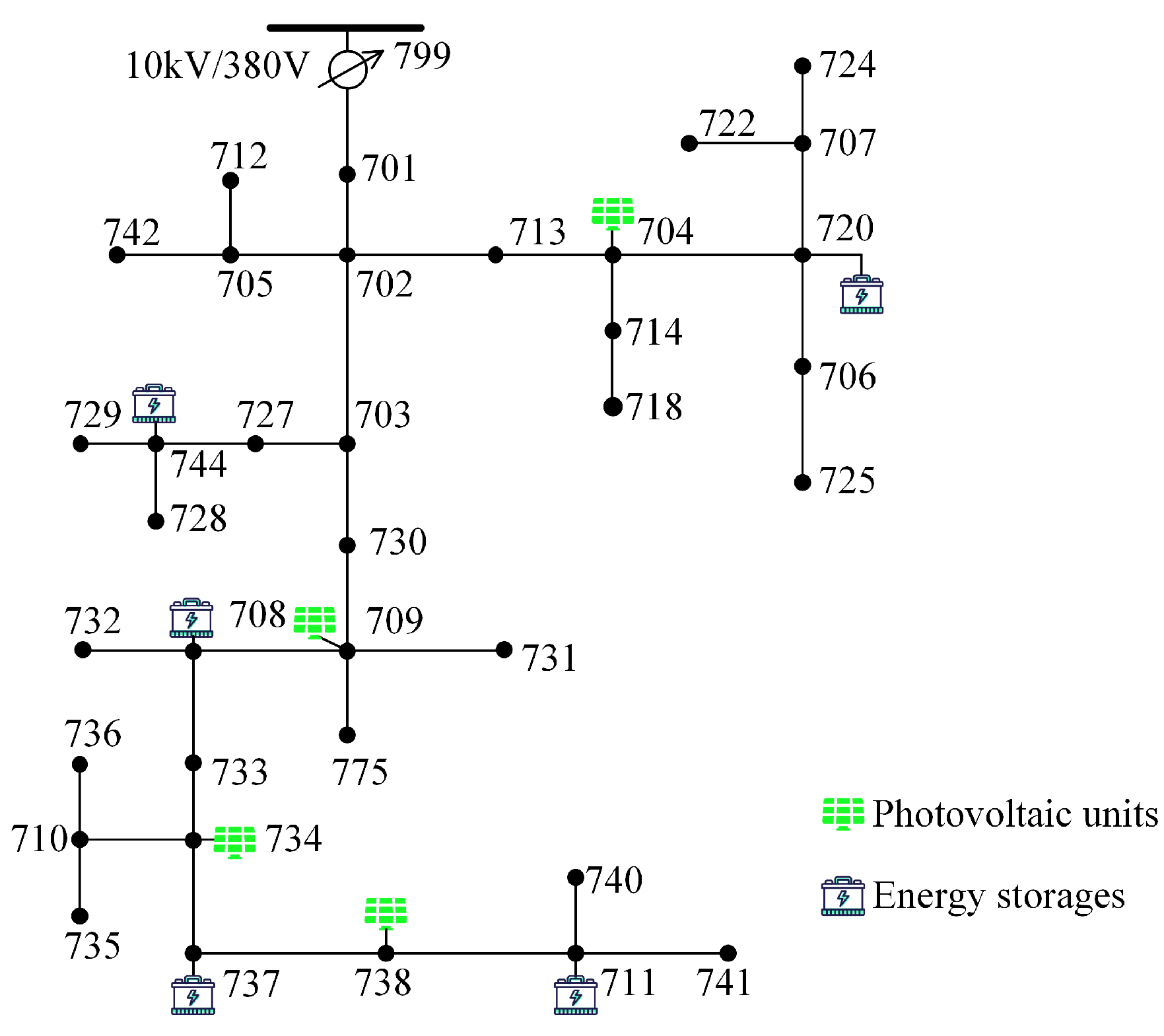
5.1. Simulation Configuration

The proposed cooperative MHE-based distributed model predictive control framework is validated in a modified 37-bus distribution network, which incorporates five energy storages (ESs) and four photovoltaic (PV) units, as illustrated in Figure 4 [21]. System parameters are detailed in

Table 1. Parameters of the test system.

Parameter	Capacity	Location	Parameter	Capacity	Location
ES1	500 kW	711	PV1	1 MW	738
ES2	500 kW	720	PV2	1 MW	734
ES3	600 kW	744	PV3	1 MW	704
ES4	600 kW	737	PV4	1 MW	709
ES5	600 kW	708

. This 37-bus system can represent a realistic distribution network to some degree, which can be employed to evaluate the efficacy of the proposed approach. The simulation is executed on MATLAB/SIMULINK R2023b software. The control sample period $T_s$, control horizon $H_c$, and prediction horizon $H_p$ of the MPC are designed, respectively, as 0.05 s, 0.5 s, and 2 s, which are necessary because 0.05 s can guarantee that the control algorithm designed in the simulation platform can run in a practical control device in real time. The parameters of control and prediction horizon in this paper can guarantee that the dynamic characteristics are considered that do not introduce unaffordable computation burden.

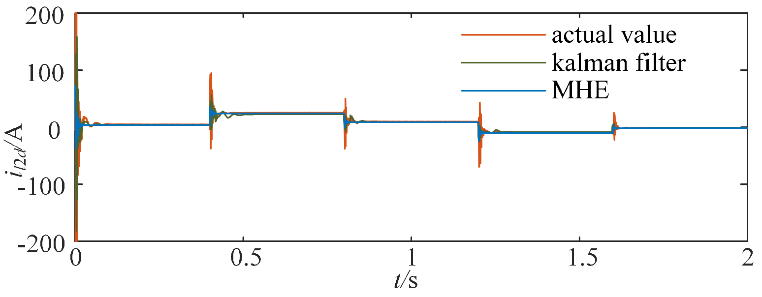
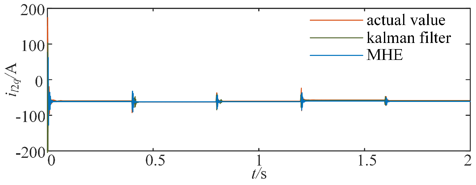
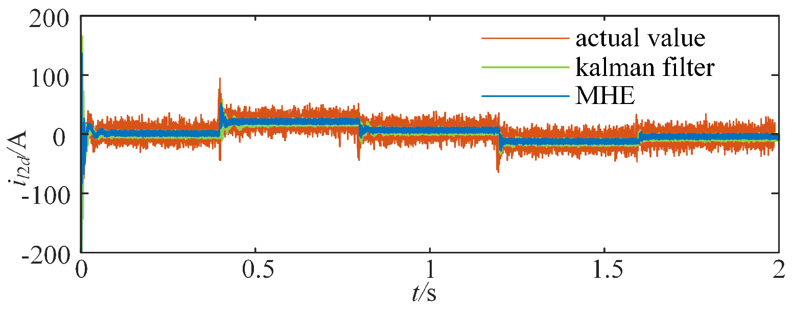
5.2. Robustness of Control Against Parameter Perturbation and Measurement Noise

In this scenario, we choose the two crucial state variables $i_{l2d},i_{l2q}$ to verify the accuracy of the feedback-linearization-based model and moving horizon estimator. Because the output current is sensitive to power disturbances, the states $i_{ld1},i_{ld2}$ can represent the interactive power between DGs and the grid. The performances of the relative methods are shown in Figure 5 and Figure 6. At t = 0.4 s, 0.8 s, 1.2 s, and 1.6 s, the DG receives a control signal, and the inner state variables start to change. The actual value changes to a new stable value within nearly 50 ms, and the MHE-based observed state variable stays within a 5% error in a dynamic process and a 1% error in a steady state. By contrast, the value observed by Kalman filter cannot achieve the same accuracy in the dynamic process, and it tends to the stable value more slowly than that based on MHE. With the observed states, the state feedback control will have better performance.

Furthermore, the robustness of MHE under parameter perturbations and measurement noise in a complex environment is demonstrated in Figure 7. In this scenario, we set the control references to change at t = 0.4 s, 0.8 s, 1.2 s, and 1.6 s in the same way. Through a comparative analysis of the actual and estimated values presented in Figure 7, the superiority of MHE over conventional methods is highlighted. Under nominal operating conditions, the MHE algorithm yields accurate approximations of the system states. Notably, in adverse measurement environments characterized by high levels of noise, the proposed approach generates smoother estimates of system states, which would significantly improve the precision of voltage control and thereby enhance the stability of voltage quality.

5.3. Voltage Control with MHE-Based MPC

To validate the proposed distributed cooperative MHE-based MPC framework in low-voltage distribution systems, random PV output perturbations are set to inject into the grid. The aggregated PV generation profile shown in Figure 8 is derived from the EPRI PV dataset and scaled down by a factor of 10 to align with the simulation time step. Specifically, power flow variations directly affect bus voltage magnitudes, making the voltage at DG-connected buses representative indicators of overall grid voltage security.

Under random power perturbations, the dynamic responses of different control strategies are compared in Figure 9, Figure 10, Figure 11 and Figure 12. The voltage variations across monitored buses closely correlate with the injected active power disturbances. Overall, the variation trend of bus voltage keeps in accordance with the injected disturbing active power. The local PI control method proposed in Section 3 exhibits voltage excursions exceeding the 1.07 p.u. upper threshold between 1.6 and 2.5 s. This is attributed to single-point feedback (voltage deviations only) lacking system-wide state awareness, rendering it inadequate for global LVDN cooperation. MPC-based controllers in Figure 10 achieve marginally better regulation, with peak voltage approaching 1.07 p.u. However, without the state estimation provided by MHE, the controller’s performance remains comparable to PI control due to insufficient system-state information. Because of the lack of crucial state variables, it is hard for the sole MPC controller to achieve great control performance. With the MHE-based distributed MPC control, the voltage level is obviously improved in this working condition. MHE-augmented distributed MPC significantly outperforms previous methods, maintaining voltage within safe limits (≤1.07 p.u.). While both non-cooperative and cooperative MPC variants demonstrate nearly identical performance, the cooperative framework achieves a marginally lower maximum voltage (1.067 p.u. vs. 1.064 p.u.), validating its superior voltage regulation capability.

5.4. Voltage Control with Cooperative MHE-Based MPC Considering Time Delay

In this section, the impact of communication delays on secondary voltage control is investigated. Figure 13 and Figure 14 compare the dynamic performances of MPC variants under a fixed 0.5 s time delay. The conventional non-cooperative MPC seen in Figure 13 exhibits instability during the simulation that voltage excursions exceeding 1.07 p.u. occur between 1.6 and 2.2 s. Furthermore, at 3.5 s and 4 s, large voltage oscillations appear during the voltage adjustment process. And, at 4 s, instability occurs in the distribution system due to its inability to handle delayed state information. On the contrary, the proposed cooperative MHE–MPC framework maintains stable operation under identical delay conditions: all bus voltages remain within the safe range (0.93–1.07 p.u.). Maximum voltage deviation is reduced by more that 40% compared to the non-cooperative MPC strategy, and smoother voltage regulation is achieved throughout the 4.5 s simulation period.

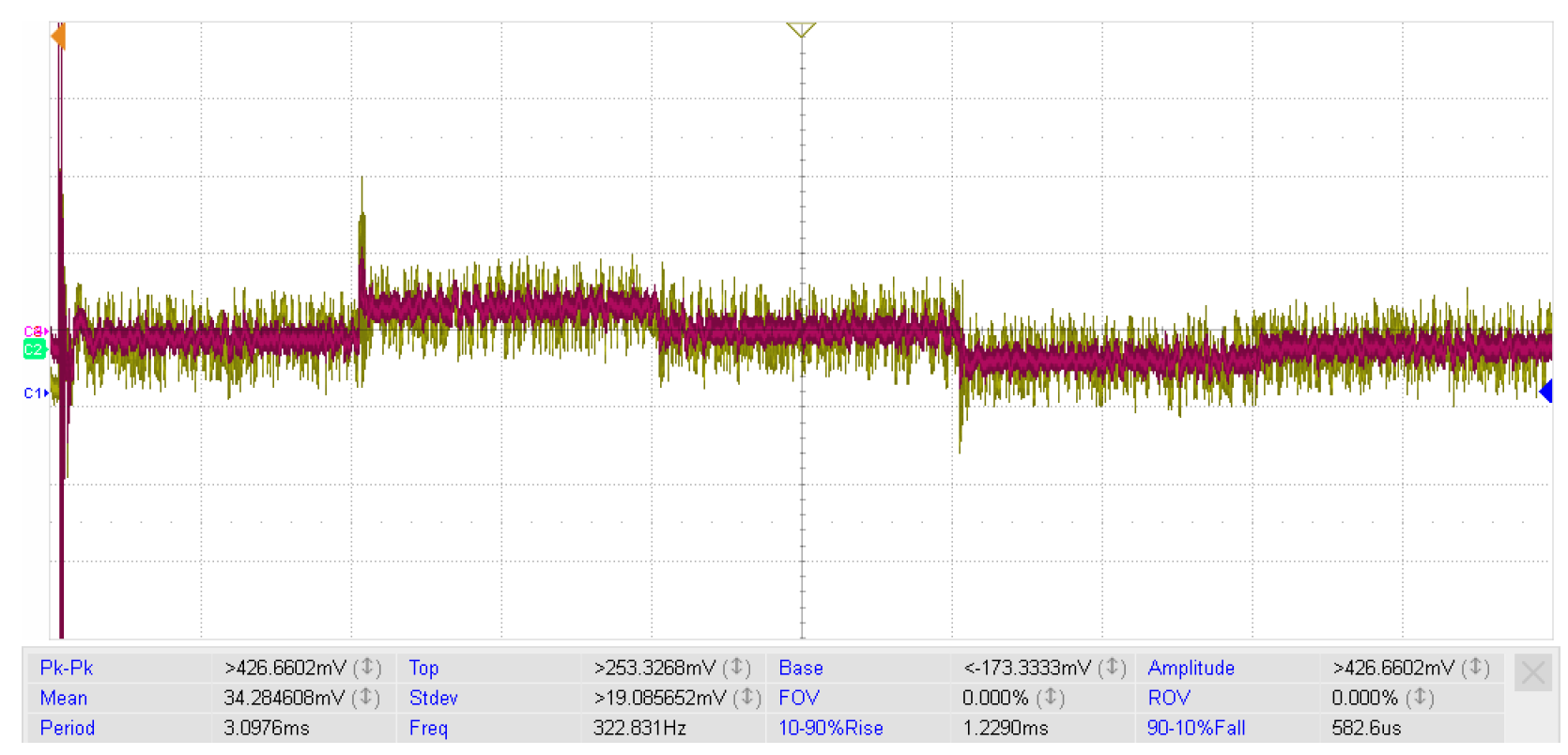
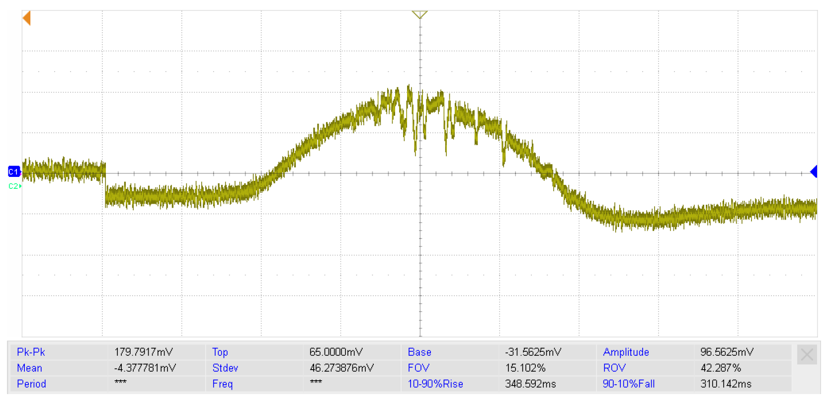
5.5. Experimental Tests

To further verify the practical feasibility of our proposed method, we test our method on an OP5700 RTLAB platform. Considering the limits of our experiment environment, we choose sectional signals to illustrate this result. As can be seen in Figure 15, we compare the actual measured current signal and the observed signal when variations happen at t = 0.4 s, 0.8 s, 1.2 s, and 1.6 s. The results illustrate that the MHE-based method can track the actual value rapidly and accurately. Meanwhile, as shown in Figure 16, we choose the maximum voltage deviation of DG 1 as an example to show that our proposed method suppresses the voltage deviations within a secure section $\pm 0.07\mathrm{p}.\mathrm{u}.$).

6. Conclusions

This paper proposes a novel MHE-based cooperative MPC method to regulate voltage in the low-voltage distribution network. After establishing the detailed DG model, we employ the feedback linearization method to simplify the detailed dynamic model of DG, which eases the difficulty in designing secondary controllers. For some unavailable variables in the feedback linearization, the MHE is introduced to obtain the necessary control data in the voltage control. Based on the above model and state information, cooperative distributed control has the foundation to realize what can adapt to poor communication in the low-voltage distribution network. Because of the inescapable time delay in the communication link, an MHE-based cooperative distributed MPC is proposed to serve the voltage control in this condition. The proposed method not only improves the voltage quality of the low-voltage distribution network but also promotes the stability of the system. However, limited by the timescale of the sample time, sectional dynamics of DGs have to be ignored, which cannot solve the narrow sample period due to the computation burden. In the future, the simplification of the control algorithms and the computation capacity of hardware devices need to be developed.

References

1. Ufa, R.; Malkova, Y.Y.; Rudnik, V.; Andreev, M.; Borisov, V. A review on distributed generation impacts on electric power system. Int. J. Hydrogen Energy 2022, 47, 20347–20361. [Google Scholar] [CrossRef]
2. Al Sumarmad, K.A.; Sulaiman, N.; Wahab, N.I.A.; Hizam, H. Energy management and voltage control in microgrids using artificial neural networks, PID, and fuzzy logic controllers. Energies 2022, 15, 303. [Google Scholar] [CrossRef]
3. Chen, N.; Du, Z.; Du, W. Optimal Regulation Strategy of Distribution Network with Photovoltaic-Powered Charging Stations Under Multiple Uncertainties: A Bi-Level Stochastic Optimization Approach. Electronics 2024, 13, 4600. [Google Scholar] [CrossRef]
4. Gallegos, J.; Arévalo, P.; Montaleza, C.; Jurado, F. Sustainable electrification—Advances and challenges in electrical-distribution networks: A review. Sustainability 2024, 16, 698. [Google Scholar] [CrossRef]
5. Le, J.; Qi, G.; Liao, X.; Zhao, L.; Jin, R. Research on voltage and power control strategy of distribution network. Int. J. Electron. 2024, 111, 204–222. [Google Scholar] [CrossRef]
6. Mumtahina, U.; Alahakoon, S.; Wolfs, P. A Day-Ahead Optimal Battery Scheduling Considering the Grid Stability of Distribution Feeders. Energies 2025, 18, 1067. [Google Scholar] [CrossRef]
7. Diahovchenko, I.; Morva, G.; Chuprun, A.; Keane, A. Comparison of voltage rise mitigation strategies for distribution networks with high photovoltaic penetration. Renew. Sustain. Energy Rev. 2025, 212, 115399. [Google Scholar] [CrossRef]
8. Guo, Y.; Fu, Y.; Li, J.; Chen, J. Optimizing Reactive Compensation for Enhanced Voltage Stability in Renewable-Integrated Stochastic Distribution Networks. Processes 2025, 13, 303. [Google Scholar] [CrossRef]
9. Sun, W.; Zhang, L.; Lv, Q.; Liu, Z.; Li, W.; Li, Q. Dynamic collaborative optimization of end-to-end delay and power consumption in wireless sensor networks for smart distribution grids. Comput. Commun. 2023, 202, 87–96. [Google Scholar]
10. Du, Y.; Lu, X.; Tang, W. Accurate Distributed Secondary Control for DC Microgrids Considering Communication Delays: A Surplus Consensus-Based Approach. IEEE Trans. Smart Grid 2022, 13, 1709–1719. [Google Scholar]
11. Srinivas, V.L.; Wu, J. Topology and Parameter Identification of Distribution Network using Smart Meter and μPMU Measurements. IEEE Trans. Instrum. Meas. 2022, 71, 9004114. [Google Scholar]
12. Zhang, J.; Wang, Y.; Weng, Y.; Zhang, N. Topology identification and line parameter estimation for non-PMU distribution network: A numerical method. IEEE Trans. Smart Grid 2020, 11, 4440–4453. [Google Scholar]
13. Matijašević Pilski, T.; Capuder, T.; Havelka, J. Identifying distribution network line parameters and voltage angles by utilizing physical knowledge: A neural network approach. Sustain. Energy Grids Netw. 2025, 41, 101606. [Google Scholar]
14. Zhang, T.; Wang, X.; Parisio, A. A corrective control framework for mitigating voltage fluctuations and congestion in distribution networks with high renewable energy penetration. Int. J. Electr. Power Energy Syst. 2025, 165, 110508. [Google Scholar]
15. Souri, S.; Shourkaei, H.M.; Soleymani, S.; Mozafari, B. Flexible reactive power management using PV inverter overrating capabilities and fixed capacitor. Electr. Power Syst. Res. 2022, 209, 107927. [Google Scholar]
16. Xu, X.; Wang, Q.; Liao, J.; Chi, Y.; Huang, T.; Zhou, N.; Zhou, Y.; Zhang, X. Static voltage stability margin evaluation for a DC distribution network with DC electric springs. Int. J. Electr. Power Energy Syst. 2025, 165, 110503. [Google Scholar]
17. alwez, M.A.; Jasni, J.; MohdRadzi, M.A.; Azis, N. Adaptive reactive power control for voltage rise mitigation on distribution network with high photovoltaic penetration. Renew. Sustain. Energy Rev. 2025, 207, 114948. [Google Scholar]
18. Mahmoodi, S.; Tarimoradi, H. A Novel Partitioning Approach in Active Distribution Networks for Voltage Sag Mitigation. IEEE Access 2024, 12, 149206–149220. [Google Scholar]
19. Rhannouch, Y.; Saadaoui, A.; Gaga, A. Analysis of the impacts of electric vehicle chargers on a medium voltage distribution network in Casablanca City. e-Prime-Adv. Electr. Eng. Electron. Energy 2025, 11, 100879. [Google Scholar]
20. Louis, A.; Ledwich, G.; Mishra, Y.; Walker, G. PQ-Based Local Voltage Regulation for Highly Resistive Radial Distribution Networks. IEEE Trans. Power Syst. 2023, 38, 4240–4251. [Google Scholar]
21. Ge, P.; Chen, B.; Teng, F. Cyber-Resilient Self-Triggered Distributed Control of Networked Microgrids Against Multi-Layer DoS Attacks. IEEE Trans. Smart Grid 2023, 14, 3114–3124. [Google Scholar]
22. Yao, W.; Wang, Y.; Xu, Y.; Deng, C.; Wu, Q. Distributed weight-average-prediction control and stability analysis for an islanded microgrid with communication time delay. IEEE Trans. Power Syst. 2021, 37, 330–342. [Google Scholar] [CrossRef]
23. Lu, X.; Lai, J. Communication constraints for distributed secondary control of heterogenous microgrids: A survey. IEEE Trans. Ind. Appl. 2021, 57, 5636–5648. [Google Scholar] [CrossRef]
24. Yang, T.; He, Y.; Liu, G.P. Distributed Voltage Restoration of AC Microgrids Under Communication Delays: A Predictive Control Perspective. IEEE Trans. Circuits Syst. I Regul. Pap. 2022, 69, 2614–2624. [Google Scholar] [CrossRef]
25. Ahumada, C.; Cárdenas, R.; Saez, D.; Guerrero, J.M. Secondary control strategies for frequency restoration in islanded microgrids with consideration of communication delays. IEEE Trans. Smart Grid 2015, 7, 1430–1441. [Google Scholar] [CrossRef]
26. Zhang, J.; Wang, J.; Yan, J.; Cheng, P. Research on multi-time scale Volt/VAR optimization in active distribution networks based on NSDBO and MPC approach. Electr. Power Syst. Res. 2025, 238, 111141. [Google Scholar] [CrossRef]
27. Lv, Y.; Dou, X.; Bu, Q.; Xu, X.; Lv, P.; Zhang, C.; Qi, Z. Tube-based MPC of hierarchical distribution network for voltage regulation considering uncertainties of renewable energy. Electr. Power Syst. Res. 2023, 214, 108875. [Google Scholar] [CrossRef]
28. Souto, L.; Parisio, A.; Taylor, P.C. MPC-based framework incorporating pre-disaster and post-disaster actions and transportation network constraints for weather-resilient power distribution networks. Appl. Energy 2024, 362, 123013. [Google Scholar] [CrossRef]
29. Song, G.; Wu, Q.; Tan, J.; Jiao, W.; Chen, J. Stochastic MPC based double-time-scale voltage regulation for unbalanced distribution networks with distributed generators. Int. J. Electr. Power Energy Syst. 2024, 155, 109687. [Google Scholar]
30. Stanojev, O.; Markovic, U.; Aristidou, P.; Hug, G.; Callaway, D.S.; Vrettos, E. MPC-based fast frequency control of voltage source converters in low-inertia power systems. IEEE Trans. Power Syst. 2020, 37, 3209–3220. [Google Scholar]
31. Ademola-Idowu, A.; Zhang, B. Frequency stability using MPC-based inverter power control in low-inertia power systems. IEEE Trans. Power Syst. 2020, 36, 1628–1637. [Google Scholar]
32. Maharjan, S.; Khambadkone, A.M.; Peng, J.C.H. Robust constrained model predictive voltage control in active distribution networks. IEEE Trans. Sustain. Energy 2020, 12, 400–411. [Google Scholar]
33. Zhang, S.; Chen, S.; Gu, W.; Lu, S.; Chung, C.Y. Dynamic optimal energy flow of integrated electricity and gas systems in continuous space. Appl. Energy 2024, 375, 124052. [Google Scholar]
34. Zhang, S.; Pan, G.; Li, B.; Gu, W.; Fu, J.; Sun, Y. Multi-Timescale Security Evaluation and Regulation of Integrated Electricity and Heating System. IEEE Trans. Smart Grid 2025, 16, 1088–1099. [Google Scholar] [CrossRef]
35. Isidori, A. Nonlinear Control Systems; Springer: Berlin/Heidelberg, Germany, 1995. [Google Scholar]
36. Khazaei, J.; Tu, Z.; Asrari, A.; Liu, W. Feedback linearization control of converters with LCL filter for weak AC grid integration. IEEE Trans. Power Syst. 2021, 36, 3740–3750. [Google Scholar]
37. Raković, S.V.; Levine, W.S. Handbook of Model Predictive Control; Springer: Berlin/Heidelberg, Germany, 2018. [Google Scholar]
Figure 1. The hierarchical control scheme.
Symmetry 17 00513 g001
Figure 2. The structure of grid-connected DG.
Symmetry 17 00513 g002
Figure 3. Principle of MHE.
Symmetry 17 00513 g003
Figure 4. Schematic of simulated power system.
Symmetry 17 00513 g004
Figure 5. Comparison between actual and measured i l 2 d .
Symmetry 17 00513 g005
Figure 6. Comparison between actual and measured i l 2 q .
Symmetry 17 00513 g006
Figure 7. Comparison between actual and measured i l 2 q with noise.
Symmetry 17 00513 g007
Figure 8. The output power of disturbing PVs.
Symmetry 17 00513 g008
Figure 9. Diagram of bus voltage with PI control.
Symmetry 17 00513 g009
Figure 10. Diagram of bus voltage with non-cooperative MPC without MHE.
Symmetry 17 00513 g010
Figure 11. Diagram of bus voltage with non-cooperative MHE-based MPC.
Symmetry 17 00513 g011
Figure 12. Diagram of bus voltage with cooperative MHE-based MPC.
Symmetry 17 00513 g012
Figure 13. Bus voltage with non-cooperative distributed MPC under delay.
Symmetry 17 00513 g013
Figure 14. Bus voltage with cooperative distributed MPC under delay.
Symmetry 17 00513 g014
Figure 15. Experimental test for estimation.
Symmetry 17 00513 g015
Figure 16. Experimental test for voltage regulation.
Symmetry 17 00513 g016