Abstract
Introducing a memristor into chaotic systems facilitates the construction of high-dimensional hyperchaotic systems. The hyperchaotic signals generated by these systems have important applications in the field of information security. A five-dimensional hyperchaotic system is constructed by introducing a memristor. Its hyperchaotic nature is discussed using phase diagrams and Lyapunov exponential diagrams. The effects of the parameters on the dynamical behavior are examined by bifurcation diagrams and Lyapunov exponential diagrams. To validate the theoretical model, an electronic circuit was designed for circuit simulation. The electronic simulation of the circuit was carried out using the Multisim simulation platform. Finally, the fixed-time projection synchronization of the system was taken into consideration. Three sets of synchronization schemes were considered and simulated. The synchronization scheme has the features of fast synchronization speed and robustness. It is potentially valuable for applications in the fields of chaotic communication and chaotic encryption.
1. Introduction
In the study of modern electronics and chaos theory, chaotic systems have attracted much attention due to their unique dynamical behavior and wide range of application prospects. Among them, hyperchaotic systems show great potential in the fields of secure communication, image encryption and chaotic control due to their higher complexity and unpredictability [1,2]. In recent years, with the rapid development of nanotechnology and material science, the emergence of a new type of nonlinear component, the memristor, has opened up a new direction for the study of chaotic systems.
A nonlinear resistor with a memory function is known as a memristor. It is a circuit device that represents the relationship between magnetic flux and charge. It was first proposed by Chua [3] in 1971. Strukov et al. [4] initially proposed substantial physical models of the memristor in 2008. Memristive circuits have also been extensively studied [5,6]. Memristor identification techniques have also continued to evolve [7]. Since the advent of nanoscale memristor devices, they have been widely studied and applied. The memristor’s ability to store the history information of the current is significant. This enables it to play a crucial role in various fields, including chaotic systems [8,9], neural networks [10,11] and nonlinear circuits [12,13,14]. A new hyperchaotic system can be constructed by introducing a memristor as a nonlinear function feedback term or replacing the original circuit resistance [15,16]. The memristor-based hyperchaotic system is a research field with broad application prospects [17,18]. Yuan et al. [19], Wan et al. [20] and Xu et al. [21] all introduced flux-controlled memristors to construct hyperchaotic systems. They considered the dynamics of the new systems and performed circuit simulations. Jia et al. [22] and Yu et al. [23] similarly introduced memristors to construct hyperchaotic systems and considered the dynamics of the new systems and FPGA implementation.
In recent years, memristors have been introduced into hyperchaotic systems to explore more complex dynamical behaviors and broader application prospects [24,25]. Wang et al. [26] introduced a flux-controlled memristor model to construct a new chaotic system. Three types of multi-stability phenomena as well as four types of transient behavior were found in the new system. It is shown that the new system with the memristor is more complex and has a wider range of applications. By combining the memory property of the memristor and the complexity of hyperchaotic systems, chaotic secure communication systems with higher security and stronger encryption capability can be designed. Luo et al. [27], Tamba et al. [28] and Yu et al. [29] have constructed hyperchaotic systems with memristors and considered secure communication, image encryption and FPGA implementations, respectively. This practical implementation showed the feasibility of deploying memristor-based hyperchaotic systems in real-world applications, such as secure communications and hardware-based cryptography. With the deepening of research and the development of technology, we believe that this field will bring us more surprises and discoveries.
The concept of projection synchronization was first introduced by Mainieri and Rehacek in 1999 [30]. Projection synchronization is a generalized type of synchronization with a variable projection scale factor. It means that the response system is synchronized with the drive system on a scale factor (projection factor). It can enhance the security of information flow to some extent. Khattar et al. [31] and Lai et al. [32] have studied the projection synchronization of the system using adaptive control methods. The synchronization stabilization time is an important metric for studying the synchronization of chaotic systems. It can describe the time required from the initiation of the chaotic synchronization process to the attainment of a stable synchronization state. To determine the stable time of the system, the conventional finite-time stability theory must depend on the initial state. To solve this problem, Polyakov proposed the concept of fixed-time stability in 2012 [33]. This stability theory does not depend on the initial state of the system. It is only related to the parameters of the system and the parameters of the controller. Therefore, the stabilization time of the system can be estimated even when the initial state is not known. This synchronization method is especially suitable for those systems where the initial state is difficult to obtain or where the synchronization state needs to be reached quickly. Wang et al. [34], Tan et al. [35] and Su et al. [36] investigated the synchronization problem of chaotic systems using fixed-time theory.
Fixed-time projection synchronization is a special type of system synchronization technique [37]. It combines the characteristics of fixed-time synchronization and projection synchronization. Fixed-time projection synchronization means that the drive system and the response system can achieve synchronization within a fixed-time range based on a scale factor. The certainty of time can facilitate practical applications. The projection scale relationship can enhance the security of information flow. Compared with the traditional asymptotic stabilization or finite-time stabilization, the fixed time projection control technique achieves an upper bound on the convergence time independent of the initial state, which is more robust and resistant to interference, which is a significant advantage in applications such as chaotic synchronization. We find that in recent years, scholars have investigated the fixed-time projection synchronization of neural network systems [38,39,40].
In this paper, we will discuss a new five-dimensional memristor-based hyperchaotic system. The article is organized as follows. Firstly, a flux-controlled memristor is introduced to construct a five-dimensional hyperchaotic system. Its dynamical properties are considered in terms of equilibrium point stability, phase diagrams and Lyapunov exponential diagrams. To further validate the theoretical constructs, electronic circuits were meticulously designed for the new hyperchaotic system. Their correctness was verified by simulation traces on an oscilloscope. The design of the electronic circuit verifies the feasibility of the quantitative equations with regard to its physical meaning. Finally, the fixed-time projection synchronization of the system is studied. Most of the studies on projection synchronization consider a constant scaling factor. There are very few studies on scaling by a certain function as a scaling factor. This approach allows us to explore a wider range of synchronization scenarios and potential applications. Therefore, both types of scaling factors are considered and analyzed comparatively. The implementation of the three sets of projection synchronization achieved the desired results through simulation. The validity of the synchronization was verified.
2. Memristor-Based Hyperchaotic System
2.1. System Description
A memristor is a nonlinear resistive element with a memory function, whose resistance state can change with the change in charge or magnetic flux passing through it, and this change can still be maintained after power failure. Introducing a memristor into a system using its special properties can generate and enhance chaotic behavior. The form of a memristor with smooth continuous cubic nonlinearity is . The following is the form of the flux-controlled memristor with a cubic nonlinear term [41].
where d and e are positive parameters, is the memductance of the memristor and is the flux through the memristor. We introduce this cubic nonlinear memristor to a four-dimensional system [42]. The constructed new five-dimensional system is shown below.
where , and v are the state variables, and and e are the constant parameters. The function serves as a model for the smooth flux-controlled memristor.
2.2. Phase Diagram and Lyapunov Exponents
The states of motion of hyperchaotic systems are usually characterized by highly complex and unpredictable trajectories in phase space. These trajectories may fill a finite region of the phase space but in a very irregular and chaotic manner. The parameters are set as and along with the initial condition of (1, 1, 1, 1, 1). The phase diagram in the , , and space of the system (2) is depicted in Figure 1. We can observe chaotic attractors.
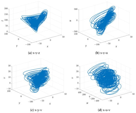
Figure 1.
The phase diagrams of the system (2) in the , , and space.
The Lyapunov exponents are an important measure of the orbital separation rate or instability of a dynamical system. In hyperchaotic systems, there are at least two positive Lyapunov exponents which correspond to the instability of the system in different directions. The Lyapunov exponential diagram of the system (2) is shown in Figure 2. The presence of two positive Lyapunov exponents indicates that the system is exhibiting a state of hyperchaos.
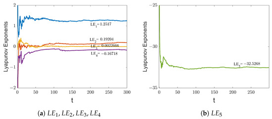
Figure 2.
The Lyapunov exponential diagram of the system (2).
The Kaplan–Yorke dimension is a concept related to the attractor dimension of a dynamical system, which is calculated based on the Lyapunov exponent of the system. The Kaplan-York dimension can be computed if there exists an integer j satisfying the conditions: and . Therefore, the calculated Kaplan–Yorke dimension of the system (2) is as follows:
The computed dimensions are non-integer, so the system has fractal dimensions. It reveals the complexity and fractal properties of chaotic attractors. The dissipativity of the system can be determined by the following equation.
Again, choosing the above parameters and initial conditions, we know that . The system is dissipative and converges at an exponential rate.
2.3. Stability of the Equilibrium Point
The equilibrium point of system (2) can be obtained by solving the following equations: . Therefore, we obtain the equilibrium point as , where . We find that a large number of equilibrium points exist. The Jacobi matrix at the equilibrium point is as follows:
We compute the corresponding characteristic polynomial at the equilibrium point as follows.
When , the equilibrium point is . The characteristic equation is . We take the parameter value as and . The five eigenvalues are . Obviously, one eigenvalue is positive, two eigenvalues are zero and the other eigenvalues are negative. Therefore, when , is an unstable saddle point.
When , the stability of the equilibrium point is determined by the Routh–Hurwitz criterion. Therefore, the equilibrium point is stable when the following conditions (7) hold.
When , and , obviously , and the above condition (7) does not hold, so the equilibrium point is unstable.
2.4. Bifurcation Analysis
The impact of the parameters on the dynamical behavior will be examined in this section. Bifurcation diagrams for hyperchaotic systems are used to demonstrate fundamental shifts in the behavior of the system dynamics as a result of a change in one or some of the parameters. In addition, as the parameters of the system change, the Lyapunov exponent changes accordingly. This change can also reflect a shift in the dynamical behavior of the system.
The bifurcation diagram and Lyapunov exponential diagram of the system (2) at are shown in Figure 3. When , the system shows chaotic behavior. As the parameter increases, two positive Lyapunov exponents can be observed in the Lyapunov exponential diagram, so the system is hyperchaotic. The bifurcation diagram of system (2) with the parameters and is shown in Figure 4. When , the system exhibits periodic motion. When the value of b increases to 40, the system (2) exhibits chaotic behavior. The phase diagram of the system (2) in the plane when we take , respectively, is shown in Figure 5. The systems in Figure 5a,b show periodic motion, and in Figure 5c the system shows chaotic motion.
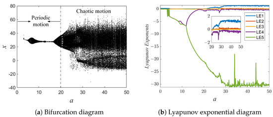
Figure 3.
The bifurcation diagram and Lyapunov exponential diagram for .
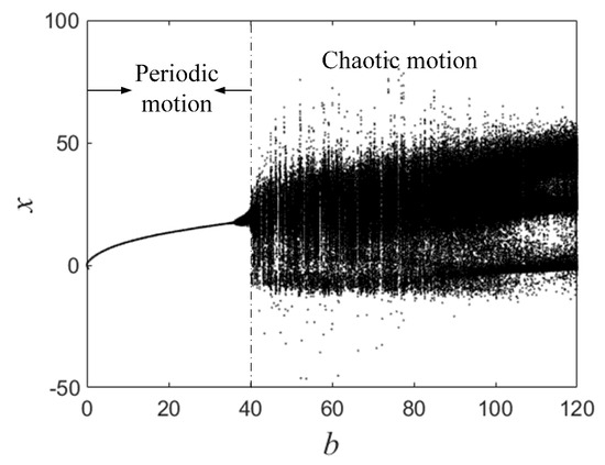
Figure 4.
The bifurcation diagram for .
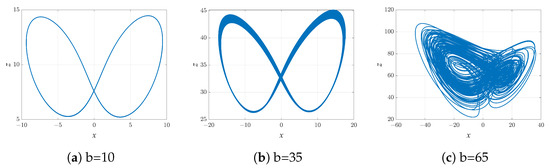
Figure 5.
Phase diagram of the system (2) in the x-z plane when and .
Consider the effect of parameter c on the system. Figure 6 illustrates the bifurcation diagram and Lyapunov exponential diagram when the parameter c is varied. We find that when , there are periodic windows in the bifurcation diagrams, such as and , and the system will experience periodic motion. It is clear that when , the system will enter a chaotic state. As shown in Figure 7, the system is in periodic motion at and and exhibits chaotic motion when .
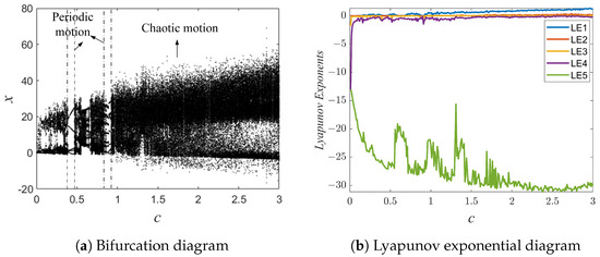
Figure 6.
The bifurcation diagram and Lyapunov exponential diagram for .
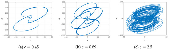
Figure 7.
Phase diagram of the system (2) in the plane when and .
In addition, we consider the effect of the parameter d on the system. When d is changed from 0 to 2, fixing the other values, the bifurcation diagram and Lyapunov exponential diagrams are as shown in Figure 8. It is seen that there is minimal impact of the parameter d on the system. The system remains in a chaotic state. Therefore, small changes in the parameter d do not significantly change the overall behavior of the system.
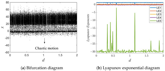
Figure 8.
The bifurcation diagram and Lyapunov exponential diagram for .
In addition, the bifurcation structure may also be affected by numerical methods. As mentioned in the literature [43,44], numerical methods also affect chaos. In numerical simulations, numerical errors may change the bifurcation structure of the system and have a significant effect on the chaotic dynamics. For example, the choice of time step (h) is crucial for the accuracy and stability of the results. Butusov et al. [45] plotted time step bifurcation maps to consider the effect of Padé 4 method and RK4 method on the system behavior. This helps us to understand the effect of numerical integration on the behavior of the system. By carefully choosing the time step and numerical integration method, we can more accurately simulate and analyze the long-term behavior of the system.
2.5. Symmetry and Coexisting Attractors
This system is symmetric and invariant to the following coordinate transformations.
Coexisting attractors in chaotic systems are a special and interesting phenomenon. Coexisting attractors refer to the phenomenon of multiple attractors of different types coexisting simultaneously in a chaotic system. Combined with the symmetry of the system, we find that picking different initial conditions creates symmetric coexisting attractors. As shown in Figure 9, the phase trajectories exhibit symmetry when the initial conditions are chosen as and . In Figure 9a, the phase trajectory in the plane x-y exhibits symmetry about the center of the origin. In Figure 9b, the phase trajectory in the plane x-z exhibits symmetry about the x-axis.
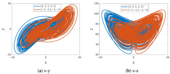
Figure 9.
The coexisting attractors of system (2) with initial values and .
3. Circuit Design and Simulation
The initial condition of capacitance in a chaotic system circuit has an important effect on the dynamical behavior of the circuit. The initial condition of a capacitor usually refers to the initial voltage or state of charge of the capacitor at the beginning of the circuit operation. Certain initial conditions may cause the circuit to enter an unstable chaotic state or fail to produce the expected chaotic behavior. We modulate the initial conditions of the circuit capacitance to ensure that the expected chaotic behavior is produced.
Based on the dimensionless equation of state, the corresponding chaotic circuits are designed using modular design concepts. The variable scale compression transformation is the first step. The operational amplifier has a linear dynamical range of V. We note that the hyperchaotic system’s state variables are outside of this range. Therefore, we must alter the state variables by compression. After the time scale transformation and letting , the state equation for the circuit simulation is as follows:
where . The values of the other parameters are given below.
Based on the analysis, we selected appropriate electronic components such as resistors, capacitors, inductors and operational amplifiers. The values of resistor R and capacitor C are shown above. The analog multipliers all have a gain of 0.1. The DC supply voltage is 15 V. The initial condition set during the simulation is zero. We designed an electronic circuit for the dimensional Equation (9). Figure 10 depicts the circuit that was designed using Mutitism 14.2. We use an oscilloscope to simulate the circuit. The phase diagram traces captured by the oscilloscope are displayed in Figure 11. The trajectories are almost the same when we compare Figure 11 with the phase diagram generated by MATLAB, which is shown in Figure 12. Therefore, the circuit design is accurate and effective. This provides a solid data basis for subsequent analysis and judgment. The results of this simulation have thus laid a solid theoretical foundation for future practical operation.
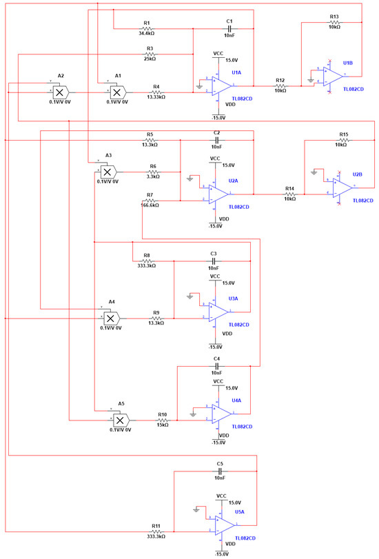
Figure 10.
Circuit model diagram of Equation (9). The initial conditions of the circuit capacitance is V.
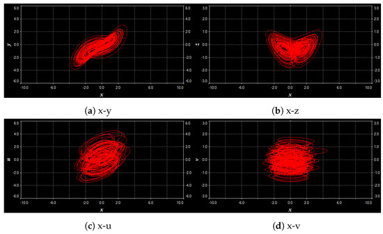
Figure 11.
Circuit simulation trajectory plots of the new five-dimensional state Equation (9) in the and planes through the oscilloscope.
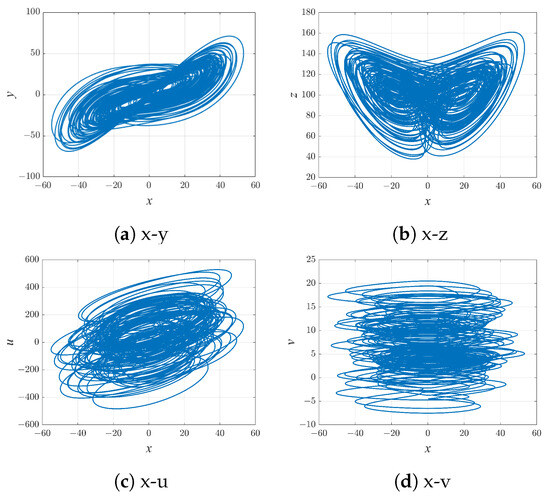
Figure 12.
Phase diagram of the system (2) in the and planes. Parameter values are and .
4. Fixed-Time Projection Synchronization
4.1. Theoretical Analysis
Consider the following two n-dimensional chaotic systems as drive and response systems, respectively:
where and are state variables, A is a linear coefficient matrix, and are nonlinear parts, and is the controller.
The function projection synchronization error is defined as . If
the function projection synchronization will be achieved between the driver and the response system, where is the scaling function and .
- The error system is acquired in this manner:
Let us also depict it as follows in a different way:
Definition 1
Definition 2
Lemma 1
([46]). Suppose is a continuous radially unbounded function that satisfies the following:
- (1):
- ;
- (2):
- any solution of the error system satisfies the following:
then the origin of system (14) can achieve fixed-time stability and the stabilization time is as follows:
where , and .
Lemma 2
([46]). If , , , the following inequality holds:
To study the fixed-time projection synchronization of drive (10) and response systems (11), we introduce controllers of the following form:
where and
Theorem 1.
Proof.
We selected the Lyapunov function as follows:
Along system (14), we compute the derivative of . Moreover, we obtain the following result by substituting (18) into the error system (14) and deflating the inequality according to Lemma 2.
where and . Let , and ; we simplify the above inequality (20) to have the following:
where , and .
The above inequality (21) satisfies the conditions of Lemma 1. Therefore, the origin of the error system (14) can achieve fixed-time stability. In addition, it follows from the inequality (20) that . Furthermore, the error vector asymptotically converges to zero, i.e., . The drive and response systems achieve fixed-time projection synchronization since the condition (12) is satisfied. According to (16), we determine that the synchronization stabilization time is . □
4.2. Numerical Simulation
We consider the following drive and response system:
Based on the above two systems, we construct the error system as follows:
In addition, according to (18), we designed the controller of the system as follows:
The following values are taken for the system’s parameters: , and . The controller’s parameters are set at and . It is assumed that the initial conditions of the drive and response systems are and . To analyze the function projection synchronization implementation, we carried out three sets of numerical simulations. The selection of the projection scale factor causes the main difference between the three sets of numerical simulations. In the following, we select three different values. We discuss the implementation of function projection synchronization by examining the error timing diagrams and the timing diagrams of the state variables.
(1) If is set as constant, projective synchronization can be achieved. When we set , the drive (22) and response (23) systems achieve projection synchronization. As demonstrated in Figure 13, the state variables of the drive (22) and response (23) systems achieve projection synchronization with projection scale of . The error state variable tends to be zero in about as shown in Figure 14. The results show that fixed-time projection synchronization is successful.
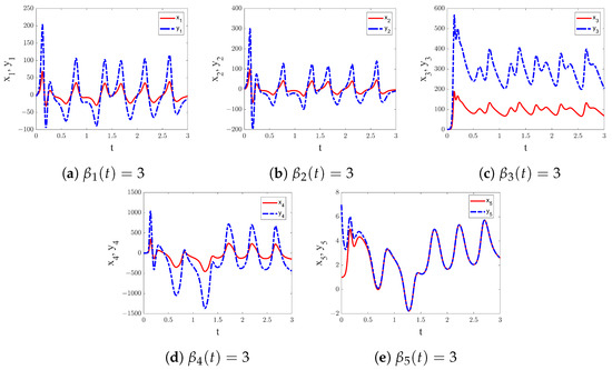
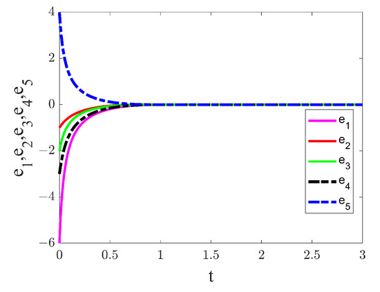
Figure 14.
The time series diagram of synchronization error and . The projection scale factor is set to .
(2) There is a unique type of projective synchronization present if or . Specifically, complete synchronization achieve if , while anti-synchronization occurs if . In addition, if the projection scale is , we call it hybrid synchronization. We consider projection scale is and . Figure 15 depicts synchronization timing diagrams for the state variables. Figure 16 displays the time series diagram of synchronization error. Thus, the drive (22) and response (23) systems achieve hybrid synchronization. We find that the system can achieve fixed-time projection synchronization in about 1 s.
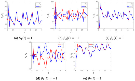
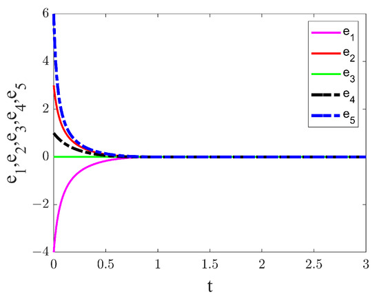
Figure 16.
The time series diagram of synchronization error and . The projection scale factor is set to and .
(3) If is defined as a function dependent on t, function projection synchronization is attained. When we take and , hybrid function projection synchronization is achieved. denotes projection along the negative direction with the projection relation increasing linearly with time; is projected along the positive direction and increases linearly with time. The timing diagram for synchronization of the state variables is displayed in Figure 17. The synchronization error variable approaches zero as Figure 18 illustrates.
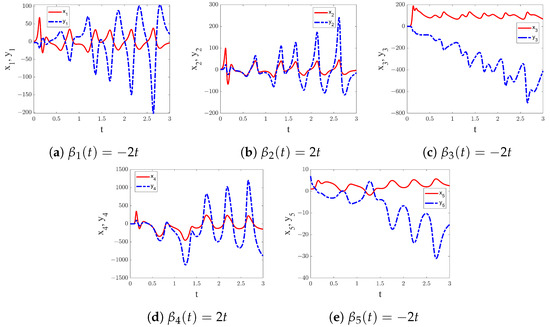
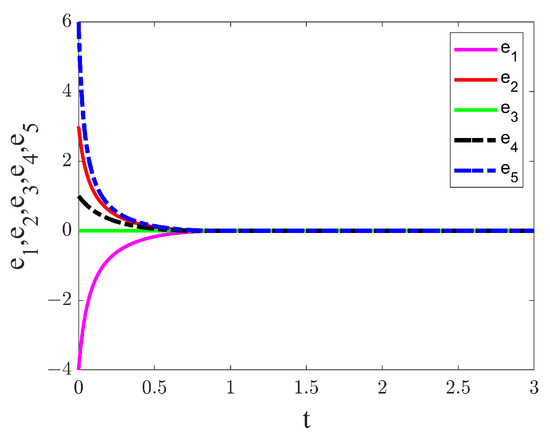
Figure 18.
The time series diagram of synchronization error and . The projection scale factor are set to and .
According to the formula given above for the synchronization stability time, we can calculate the stabilization time to achieve synchronization as s. The advantage of fixed-time synchronization is that it is not affected by initial conditions. The results of all three sets of numerical simulations indicate successful fixed-time projection synchronization. Therefore, the controller selection is reasonable and the synchronization scheme is feasible.
5. Conclusions
A flux-controlled memristor is introduced to construct a new five-dimensional hyperchaotic system. The memristor-based systems exhibit richer nonlinear behaviors. The dynamical behavior of the system is examined using phase diagrams, Lyapunov exponential diagrams and bifurcation diagrams. The effect of parameters on the system is indicated by the bifurcation diagram. When the parameters are changed, the system may enter a periodic state or chaotic state. The parameter d has little effect on the system when varied within a certain range, which is always chaotic.
We translated the system into a physical model and designed the electronic circuits. The simulated traces generated by the circuit through an oscilloscope agree with the phase diagram traces obtained from MATLAB 2021a simulation. The circuit simulation results show the correctness of the electronic circuit design. This implies the potential feasibility and physical significance of the system in practical applications. Finally, fixed-time projection synchronization between systems is considered in conjunction with fixed-time stability theory and projection synchronization. Three cases of synchronization simulations are considered where the projection scale factor is taken to be constant, and as a function of time, respectively. The synchronization timing diagrams and error diagrams generated from these simulations provide compelling evidence for the efficacy and robustness of the synchronization method employed.
Author Contributions
Conceptualization, Y.Z.; Investigation, R.L.; Formal analysis, Y.Z.; Software, R.L.; Writing—original draft, R.L.; Writing—review and editing, Z.C.; Funding acquisition, Y.Z. All authors have read and agreed to the published version of the manuscript.
Funding
The authors gratefully acknowledge the support of the National Natural Science Foundation of China (12462004, 12262024), the Fundamental Research Funds for the Inner Mongolia Normal University (2023JBBJ004) and the Project Supported by Natural Science Foundation of Inner Mongolia Autonomous Region (2022MS01003).
Data Availability Statement
Data are contained within the article.
Conflicts of Interest
The authors declare no conflict of interest.
References
- Sheela, S.J.; Sanjay, A.; Suresh, K.V.; Tandur, D.; Shubha, G. Image encryption based on 5D hyperchaotic system using hybrid random matrix transform. Multidimens. Syst. Signal Process. 2022, 33, 579–595. [Google Scholar] [CrossRef]
- Gómez, J.C.G.; dos Santos, R.R.; Gularte, K.H.M.; Vargas, J.A.R.; Hernández, J.A.R. A Robust Underactuated Synchronizer for a Five-dimensional Hyperchaotic System: Applications for Secure Communication. Int. J. Control Autom. Syst. 2023, 21, 2891–2903. [Google Scholar] [CrossRef]
- Chua, L. Memristor-the missing circuit element. IEEE Trans. Circuit Theory 1971, 18, 507–519. [Google Scholar] [CrossRef]
- Strukov, D.B.; Snider, G.S.; Stewart, D.R.; Williams, R.S. The missing memristor found. Nature 2008, 453, 80–83. [Google Scholar] [CrossRef]
- Butusov, D.N.; Karimov, A.I.; Pesterev, D.O.; Tutueva, A.V.; Okoli, G. Bifurcation and recurrent analysis of memristive circuits. In Proceedings of the 2018 IEEE Conference of Russian Young Researchers in Electrical and Electronic Engineering (EIConRus), Moscow, Russia, 29 January–1 February 2018; pp. 178–183. [Google Scholar]
- Ostrovskii, V.Y.; Tutueva, A.V.; Rybin, V.G.; Karimov, A.I.; Butusov, D.N. Continuation analysis of memristor-based modified Chua’s circuit. In Proceedings of the 2020 International Conference Nonlinearity, Information and Robotics (NIR), Innopolis, Russia, 3–6 December 2020; pp. 1–5. [Google Scholar]
- Ostrovskii, V.; Fedoseev, P.; Bobrova, Y.; Butusov, D. Structural and Parametric Identification of Knowm Memristors. Nanomaterials 2022, 12, 63. [Google Scholar] [CrossRef]
- Wu, X.M.; He, S.B.; Tan, W.J.; Wang, H.H. From memristor-modeled jerk system to the nonlinear systems with memristor. Symmetry 2022, 14, 659. [Google Scholar] [CrossRef]
- Zhou, L.; Wang, C.; Zhou, L. Generating four-wing hyperchaotic attractor and two-wing, three-wing, and four-wing chaotic attractors in 4D memristive system. Int. J. Bifurc. Chaos 2017, 27, 1750027. [Google Scholar] [CrossRef]
- Pham, V.T.; Jafari, S.; Vaidyanathan, S.; Volos, C.; Wang, X. A novel memristive neural network with hidden attractors and its circuitry implementation. Sci. China Technol. Sci. 2016, 59, 358–363. [Google Scholar] [CrossRef]
- Zhang, Z.; Li, C.; Zhang, W.; Zhou, J.; Liu, G. An FPGA-based memristor emulator for artificial neural network. Microelectron. J. 2023, 131, 105639. [Google Scholar] [CrossRef]
- Bao, B.C.; Ma, Z.H.; Xu, J.P.; Liu, Z.; Xu, Q. A simple memristor chaotic circuit with complex dynamics. Int. J. Bifurc. Chaos 2011, 21, 2629–2645. [Google Scholar] [CrossRef]
- Wang, C.H.; Zhou, L.; Wu, R.P. The design and realization of a hyper-chaotic circuit based on a flux-controlled memristor with linear memductance. J. Circuits Syst. Comput. 2018, 27, 1850038. [Google Scholar] [CrossRef]
- Messadi, M.; Kemih, K.; Moysis, L.; Volos, C. A new 4D Memristor chaotic system: Analysis and implementation. Integration 2023, 88, 91–100. [Google Scholar] [CrossRef]
- Zhou, L.; Wang, C.; Zhou, L. Generating hyperchaotic multi-wing attractor in a 4D memristive circuit. Nonlinear Dyn. 2016, 85, 2653–2663. [Google Scholar]
- Wang, C.H.; Xia, H.; Zhou, L. A memristive hyperchaotic multiscroll jerk system with controllable scroll numbers. Int. J. Bifurc. Chaos 2017, 27, 1750091. [Google Scholar]
- Luo, J.; Tang, W.T.; Chen, Y.; Chen, X.; Zhou, H. Dynamical analysis and synchronization control of flux-controlled memristive chaotic circuits and its FPGA-Based implementation. Results Phys. 2023, 54, 107085. [Google Scholar]
- Chen, Q.; Li, B.; Yin, W.; Jiang, X.W.; Chen, X.Y. Bifurcation, chaos and fixed-time synchronization of memristor cellular neural networks. Chaos Solitons Fractals 2023, 171, 113440. [Google Scholar]
- Yuan, F.; Wang, G.Y.; Wang, X.W. Extreme multistability in a memristor-based multi-scroll hyper-chaotic system. Chaos 2016, 26, 073107. [Google Scholar] [CrossRef]
- Wan, Q.Z.; Li, F.; Yan, Z.D.; Chen, S.M.; Liu, J.; Ji, W.K.; Yu, F. Dynamic analysis and circuit realization of a novel variable-wing 5D memristive hyperchaotic system with line equilibrium. Eur. Phys. J. Spec. Top. 2022, 231, 3029–3041. [Google Scholar] [CrossRef]
- Xu, C.B.; Luo, Y.T.; Li, X.Y.; Fan, C.L. A novel 5D memristor conservative chaotic system with multiple forms of hidden flows. Phys. Scr. 2023, 99, 015243. [Google Scholar]
- Jia, S.H.; Li, Y.X.; Shi, Q.Y.; Huang, X. Design and FPGA implementation of a memristor-based multi-scroll hyperchaotic system. Chin. Phys. B 2022, 31, 070505. [Google Scholar] [CrossRef]
- Yu, F.; Zhang, W.X.; Xiao, X.L.; Yao, W.; Cai, S.; Zhang, J.; Wang, C.H.; Li, Y. Dynamic analysis and FPGA implementation of a new, simple 5D memristive hyperchaotic Sprott-C system. Mathematics 2023, 11, 701. [Google Scholar] [CrossRef]
- Min, X.T.; Wang, X.Y.; Zhou, P.F.; Yu, S.M.; Iu, H.H.C. An optimized memristor-based hyperchaotic system with controlled hidden attractors. IEEE Access 2019, 7, 124641–124646. [Google Scholar] [CrossRef]
- Li, X.X.; Liu, D.J.; Zheng, C.; Xue, X.P.; Xu, G.Z. Symmetric extreme multistability and memristor initial-offset boosting in a new 5D four-wing hyperchaotic system based on dual memristors. Mod. Phys. Lett. B 2022, 36, 2250090. [Google Scholar] [CrossRef]
- Wang, Q.; Hu, C.Y.; Tian, Z.; Wu, X.M.; Sang, H.W.; Cui, Z.W. A 3D memristor-based chaotic system with transition behaviors of coexisting attractors between equilibrium points. Results Phys. 2024, 56, 107201. [Google Scholar] [CrossRef]
- Luo, J.; Qu, S.C.; Chen, Y.; Chen, X.; Xiong, Z.L. Synchronization, circuit and secure communication implementation of a memristor-based hyperchaotic system using single input controller. Chin. J. Phys. 2021, 71, 403–417. [Google Scholar] [CrossRef]
- Tamba, V.K.; Biamou, A.L.M.; Tagne, F.K.; Takougang, A.C.N.; Fotsin, H.B. Hidden extreme multistability in a smooth flux-controlled memristor based four-dimensional chaotic system and its application in image encryption. Phys. Scr. 2024, 99, 025210. [Google Scholar] [CrossRef]
- Yu, F.; Xu, S.; Xiao, X.L.; Yao, W.; Huang, Y.Y.; Cai, S.; Yin, B.; Li, Y. Dynamics analysis, FPGA realization and image encryption application of a 5D memristive exponential hyperchaotic system. Integration 2023, 90, 58–70. [Google Scholar] [CrossRef]
- Mainieri, R.; Rehacek, J. Projective synchronization in three-dimensional chaotic systems. Phys. Rev. Lett. 1999, 82, 3042. [Google Scholar] [CrossRef]
- Khattar, D.; Agrawal, N.; Sirohi, M. Dynamical analysis of a 5D novel system based on Lorenz system and its hybrid function projective synchronisation using adaptive control. Pramana J. Phys. 2023, 97, 76. [Google Scholar] [CrossRef]
- Lai, Q.; Wang, Z.L. Finite-time projective synchronization of complex networks via adaptive control. Indian J. Phys. 2023, 97, 3617–3628. [Google Scholar] [CrossRef]
- Polyakov, A. Nonlinear feedback design for fixed-time stabilization of linear control systems. IEEE Trans. Autom. Control 2011, 57, 2106–2110. [Google Scholar] [CrossRef]
- Wang, H.Q.; Ai, Y.D. Adaptive fixed-time control and synchronization for hyperchaotic Lü systems. Appl. Math. Comput. 2022, 433, 127388. [Google Scholar] [CrossRef]
- Tan, Z.L.; Sun, J.Y.; Zhang, H.G.; Xie, X.P. Chaos synchronization control for stochastic nonlinear systems of interior PMSMs based on fixed-time stability theorem. Appl. Math. Comput. 2022, 430, 127115. [Google Scholar] [CrossRef]
- Su, H.P.; Luo, R.Z.; Fu, J.J.; Huang, M.C. Fixed time control and synchronization of a class of uncertain chaotic systems with disturbances via passive control method. Math. Comput. Simul. 2022, 198, 474–493. [Google Scholar] [CrossRef]
- Bekiros, S.; Yao, Q.J.; Mou, J.; Alkhateeb, A.F.; Jahanshahi, H. Adaptive fixed-time robust control for function projective synchronization of hyperchaotic economic systems with external perturbations. Chaos Solitons Fractals 2023, 172, 113609. [Google Scholar] [CrossRef]
- Chen, C.; Li, L.X.; Peng, H.P.; Yang, Y.X.; Mi, L.; Qiu, B.L. Fixed-time projective synchronization of memristive neural networks with discrete delay. Phys. A Stat. Mech. Its Appl. 2019, 534, 122248. [Google Scholar] [CrossRef]
- Xiao, L.; Li, L.J.; Cao, P.L.; He, Y.J. A fixed-time robust controller based on zeroing neural network for generalized projective synchronization of chaotic systems. Chao Solitons Fractals 2023, 169, 113279. [Google Scholar] [CrossRef]
- Hao, C.Q.; Wang, B.X.; Tang, D.D. Finite-time and fixed-time function projective synchronization of competitive neural networks with noise perturbation. Neural Comput. Appl. 2024, 36, 16527–16543. [Google Scholar] [CrossRef]
- Sun, J.W.; Yao, L.N.; Zhang, X.C.; Wang, Y.F.; Cui, G.Z. Generalised mathematical model of memristor. IET Circuits Devices Syst. 2016, 10, 244–249. [Google Scholar] [CrossRef]
- Hu, Y.M.; Lai, B.C. Generating coexisting attractors from a new four-dimensional chaotic system. Mod. Phys. Lett. B 2021, 35, 2150035. [Google Scholar] [CrossRef]
- Corless, R.M.; Essex, C.; Nerenberg, M.A.H. Numerical methods can suppress chaos. Phys. Lett. A 1991, 157, 27–36. [Google Scholar] [CrossRef]
- Ostrovskii, V.Y.; Rybin, V.G.; Karimov, A.I.; Butusov, D.N. Inducing multistability in discrete chaotic systems using numerical integration with variable symmetry. Chaos Solitons Fractals 2022, 165, 112794. [Google Scholar] [CrossRef]
- Butusov, D.; Karimov, A.; Tutueva, A.; Kaplun, D.; Nepomuceno, E.G. The effects of Padé numerical integration in simulation of conservative chaotic systems. Entropy 2019, 21, 362. [Google Scholar] [CrossRef] [PubMed]
- Chen, C.; Li, L.X.; Peng, H.P.; Yang, Y.X.; Mi, L.; Zhao, H. A new fixed-time stability theorem and its application to the fixed-time synchronization of neural networks. Neural Netw. 2020, 123, 412–419. [Google Scholar] [CrossRef]
Disclaimer/Publisher’s Note: The statements, opinions and data contained in all publications are solely those of the individual author(s) and contributor(s) and not of MDPI and/or the editor(s). MDPI and/or the editor(s) disclaim responsibility for any injury to people or property resulting from any ideas, methods, instructions or products referred to in the content. |
© 2025 by the authors. Licensee MDPI, Basel, Switzerland. This article is an open access article distributed under the terms and conditions of the Creative Commons Attribution (CC BY) license (https://creativecommons.org/licenses/by/4.0/).