
Symbol Recognition Method for Railway Catenary Layout Drawings Based on Deep Learning


Abstract
1. Introduction
- Improve the baseline model YOLOv8n, then sequentially introduce MSDA, RFAConv, and Dysample to improve the feature extraction ability and small target identification effect in difficult scenarios.
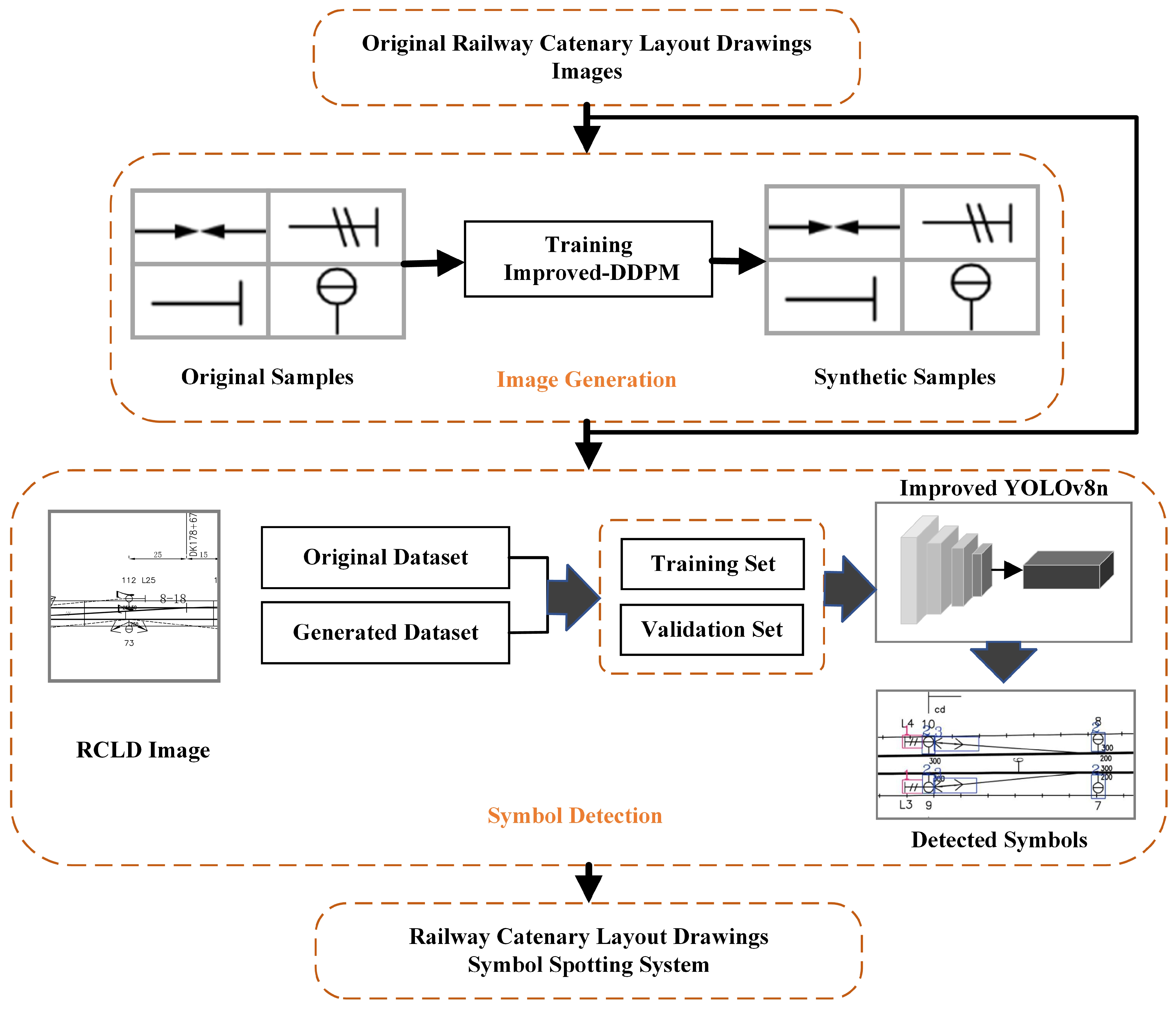
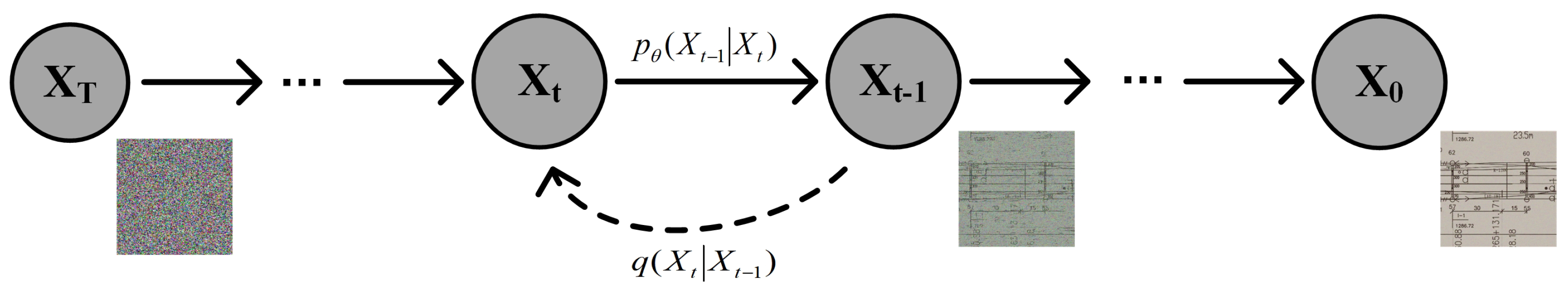
- Differing from traditional GAN-based sample generation methods, this paper introduces IDDPM for symbol recognition in RCLDs. This generates higher-quality, more stable samples for minority classes, helping to alleviate category imbalances and enhance recognition performance for minority symbols.
- Based on the improved YOLOv8n model, the original dataset and the dataset with the addition of synthetic data are trained separately to evaluate the detection performance and perform a comprehensive analysis and comparison.
2. Related Work
2.1. Development of Object Detection Algorithms
2.2. Symbol Detection Methods Using Engineering Drawings
2.3. Synthetic Image Methods Using Engineering Drawings
3. Methodology
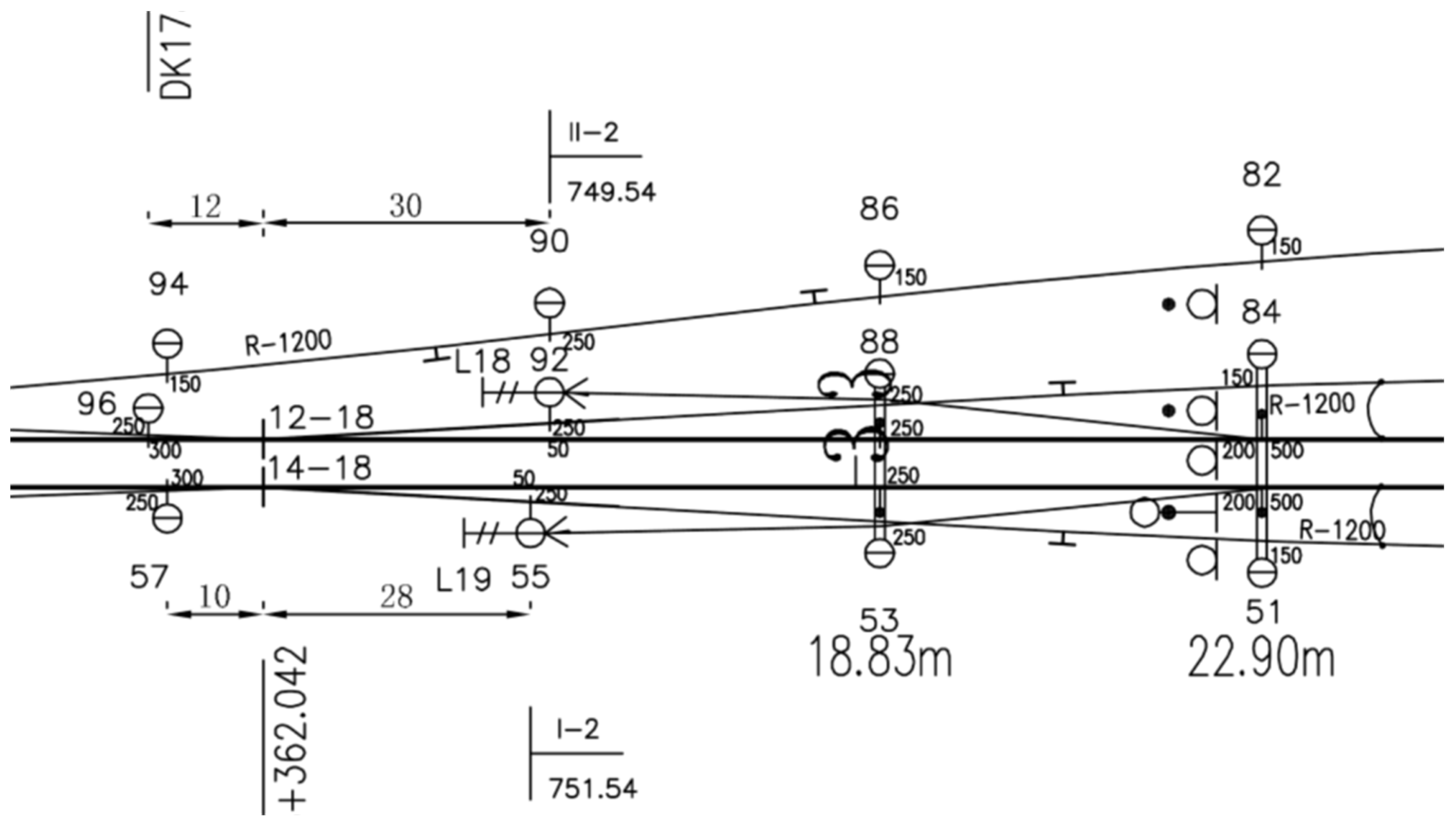
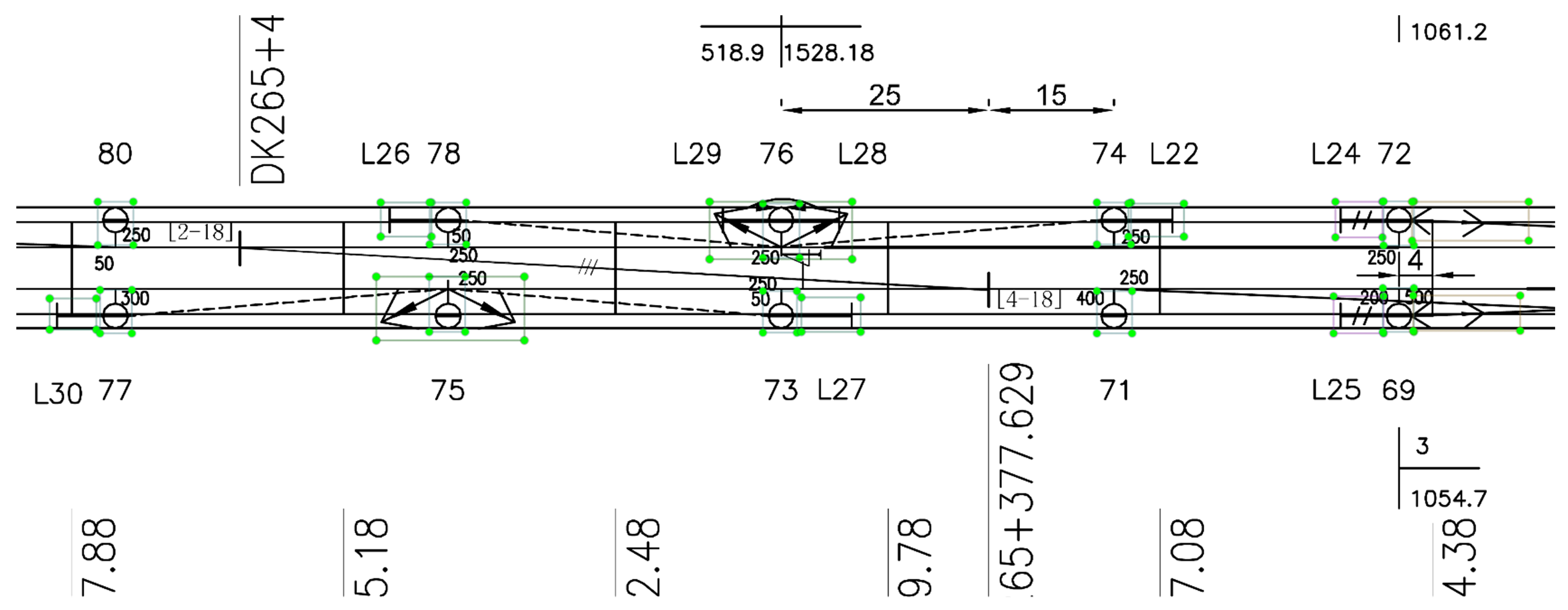
3.1. RCLDs Dataset
3.2. Symbol Recognition Methods
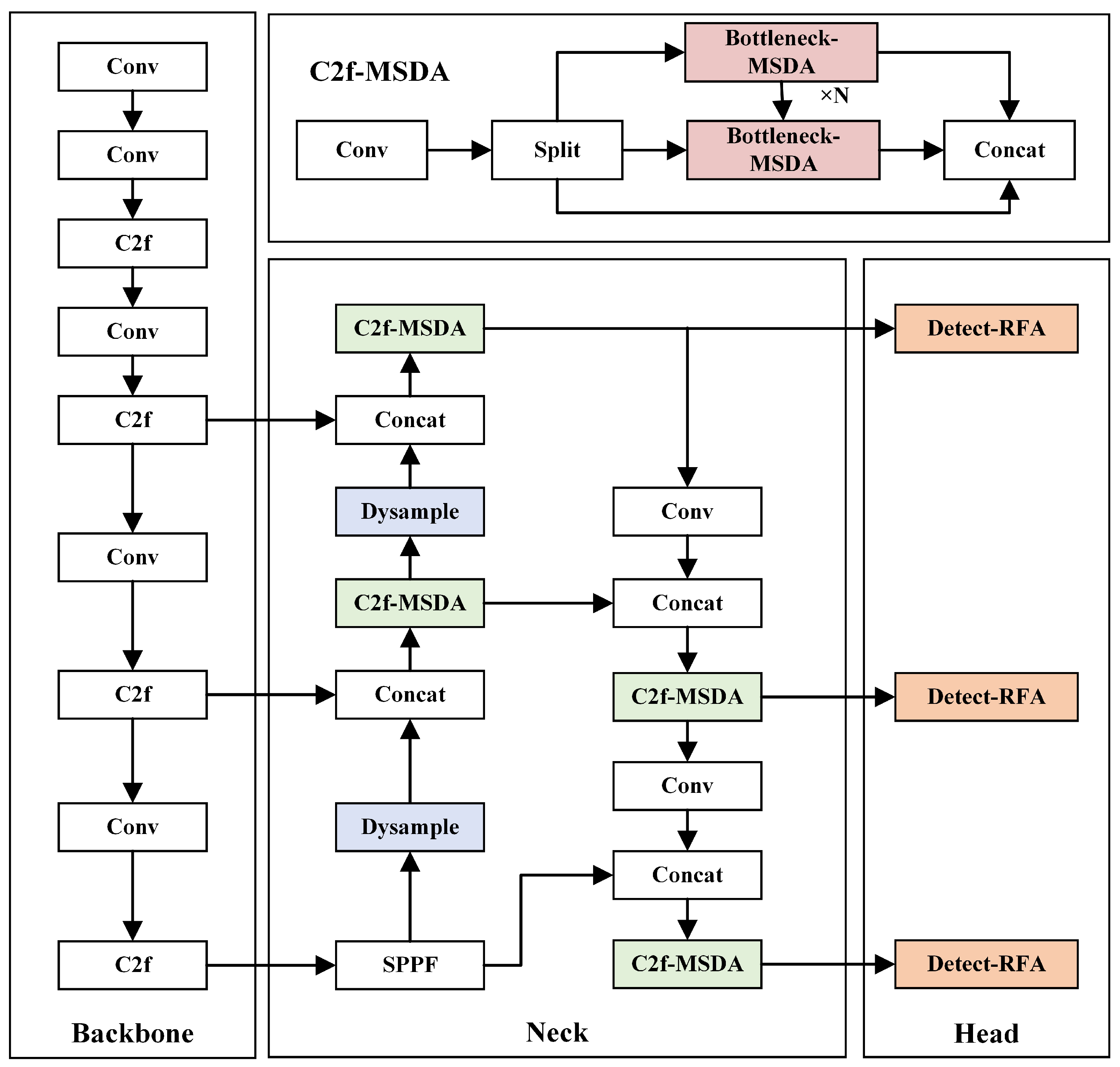
3.3. Improved YOLOV8n
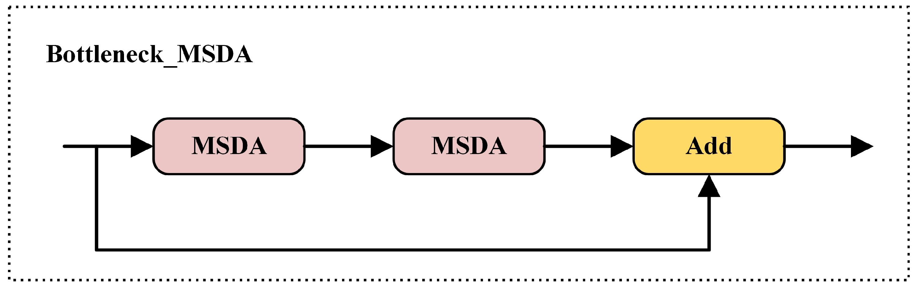
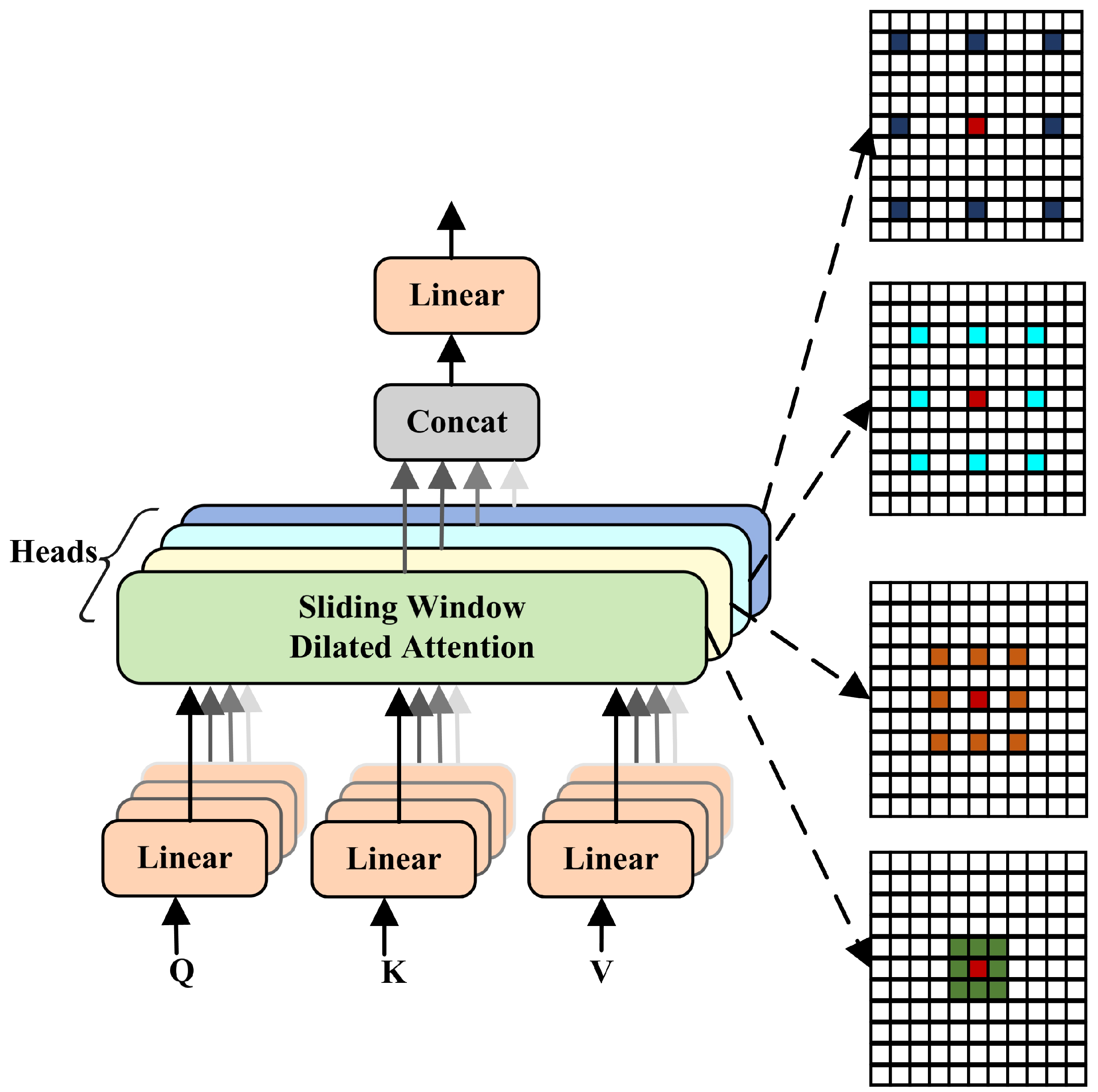
3.3.1. C2f-MSDA
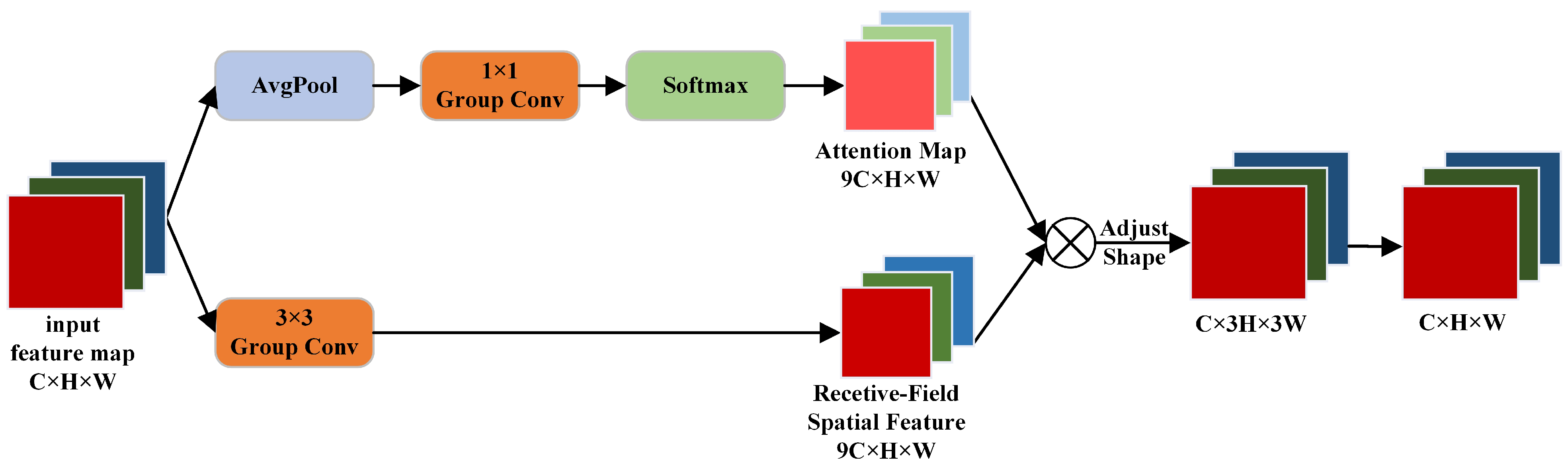
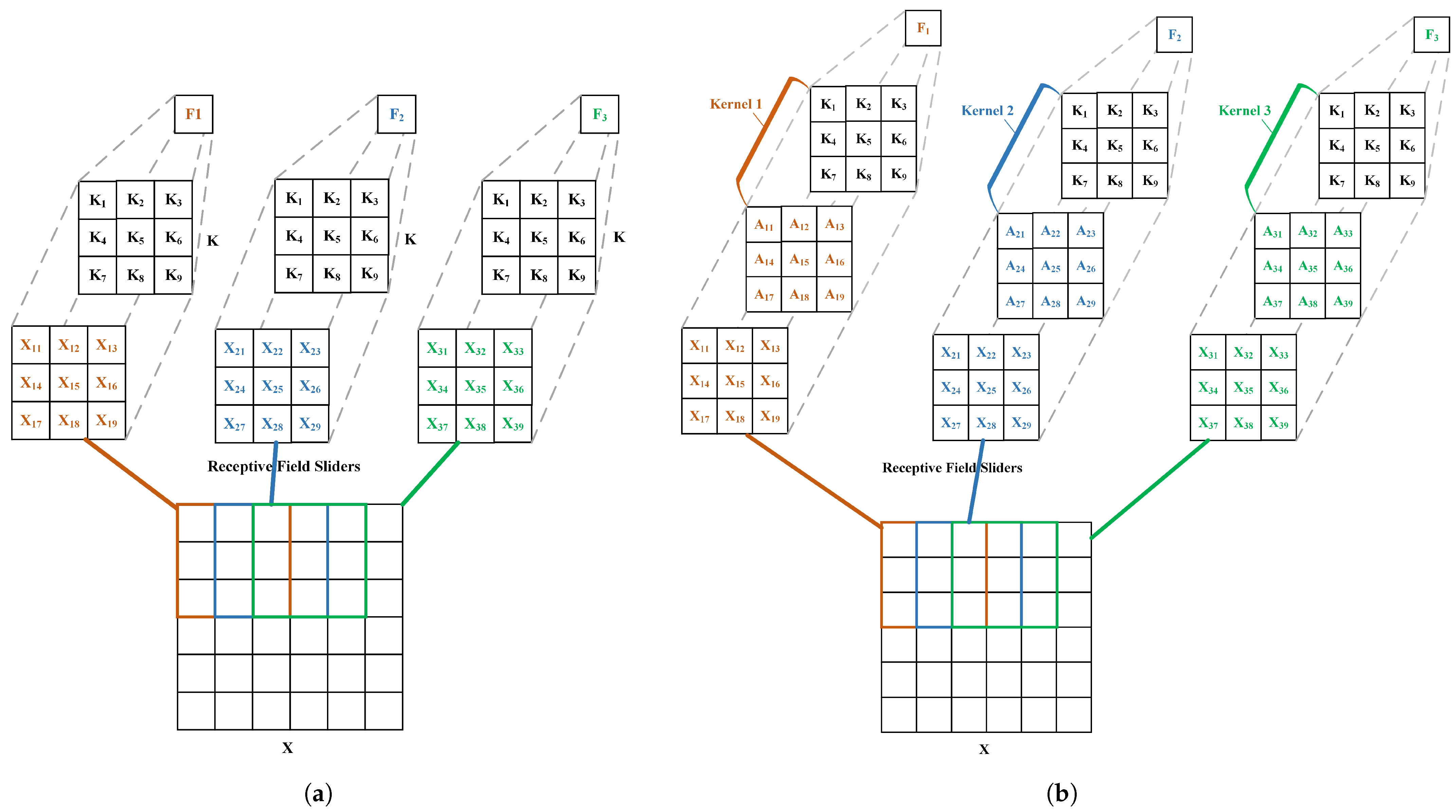
3.3.2. Detect RFA
3.3.3. Dysample
3.4. IDDPM Generates Synthetic Images
4. Experiments
4.1. Evaluation of the Improved YOLOv8n
4.1.1. Experimental Environment
4.1.2. Data Preprocessing
4.1.3. Evaluation Metrics
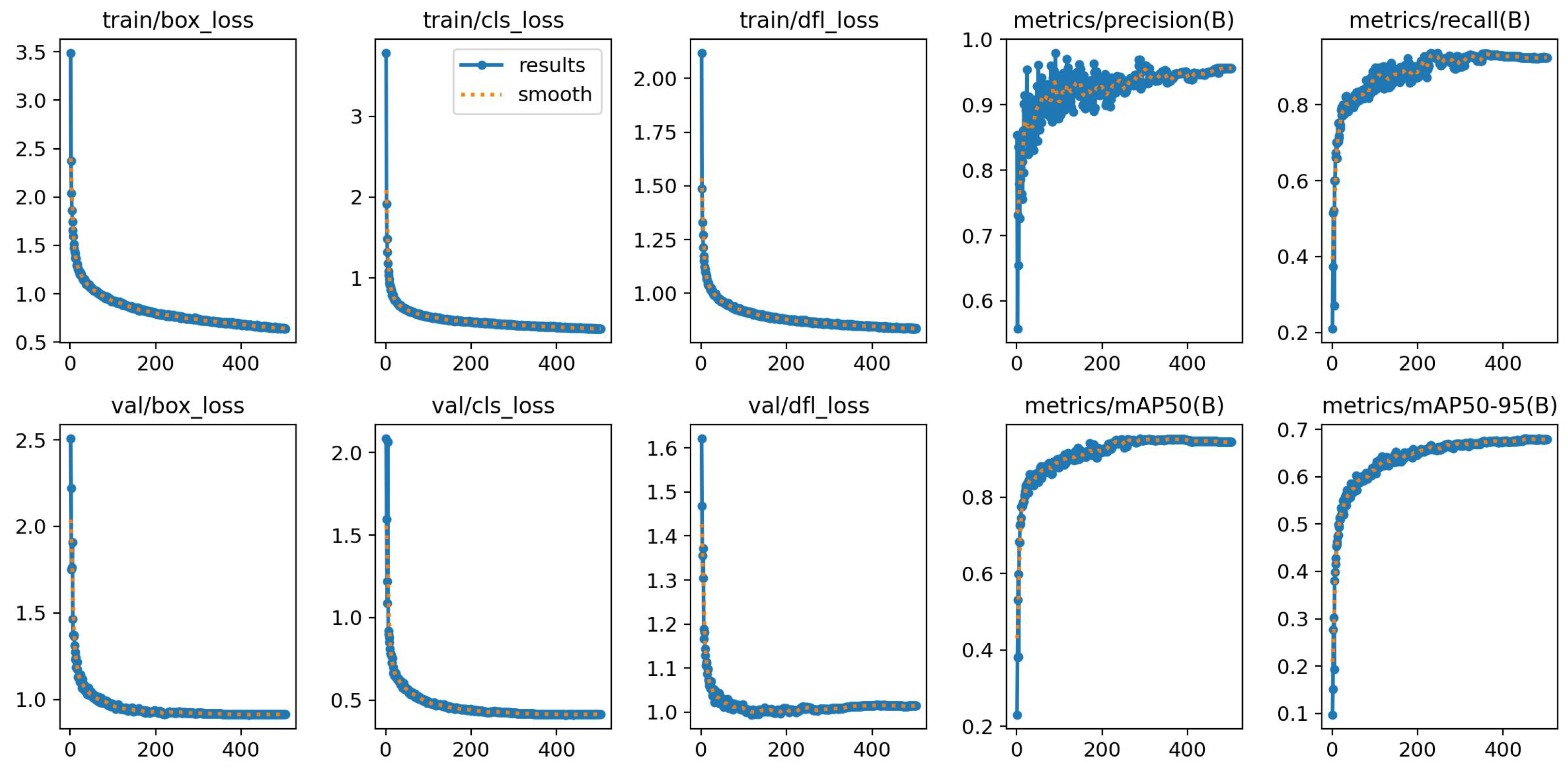
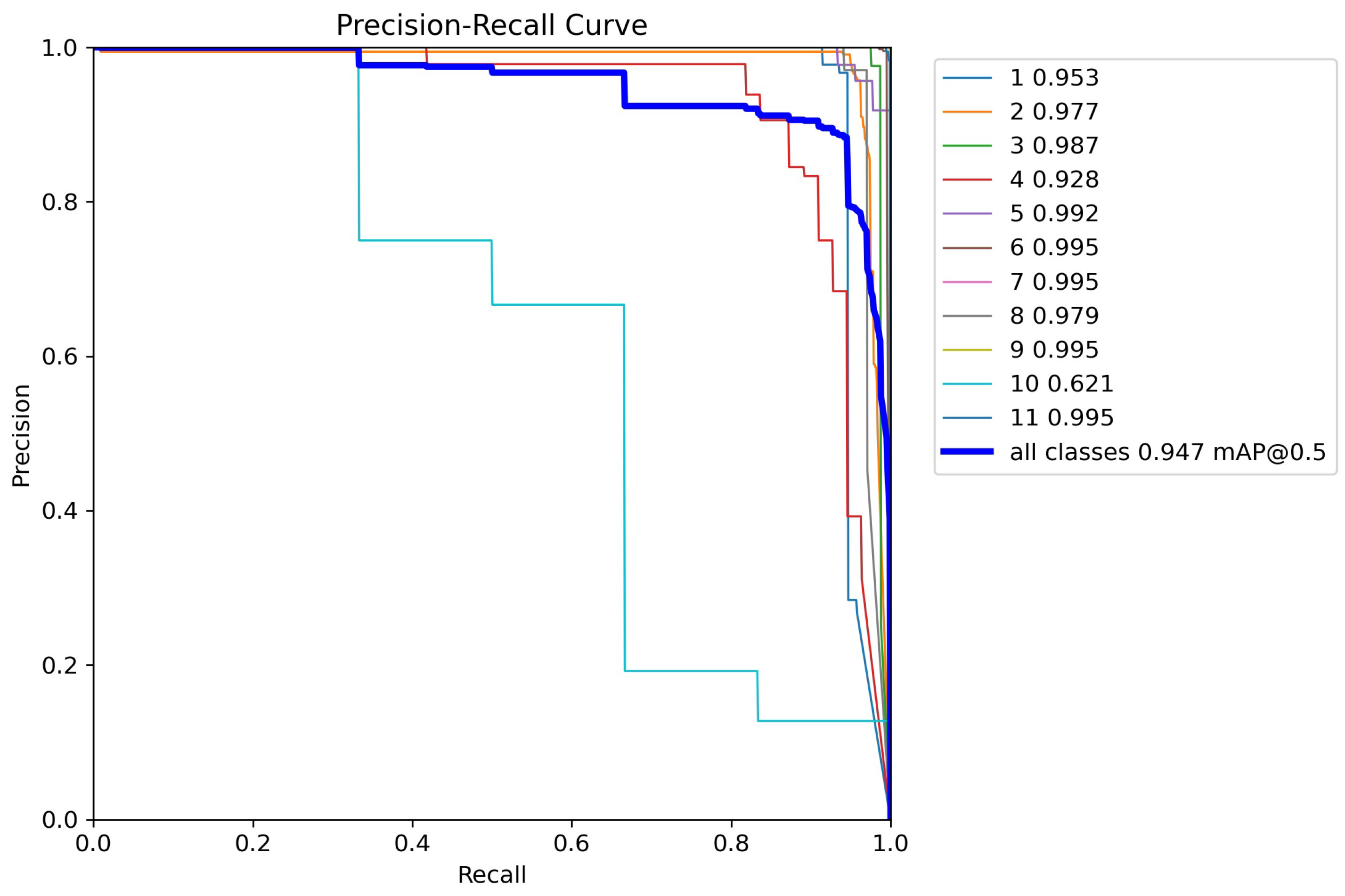
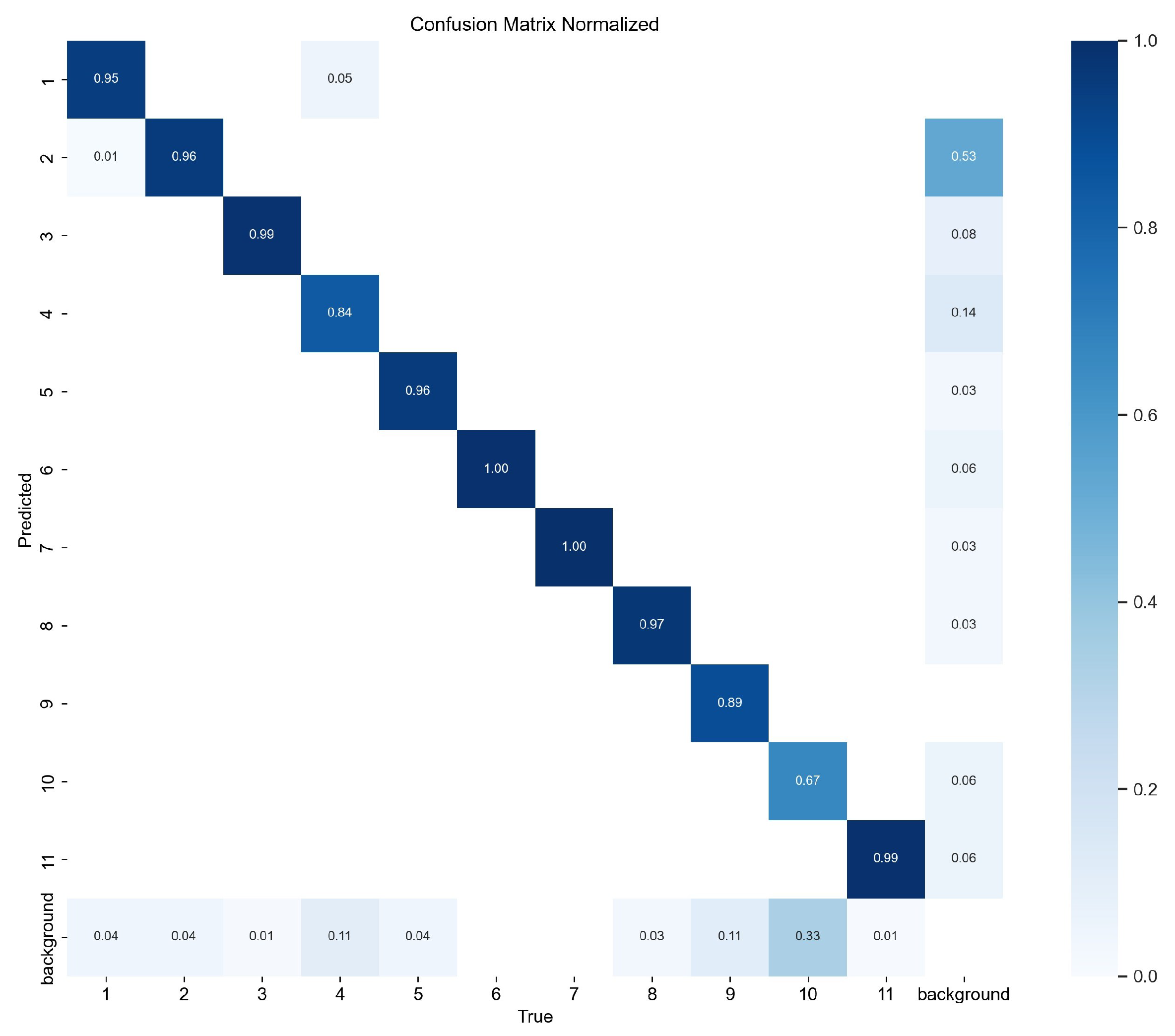
4.1.4. Improved YOLOv8n Experimental Results Analysis
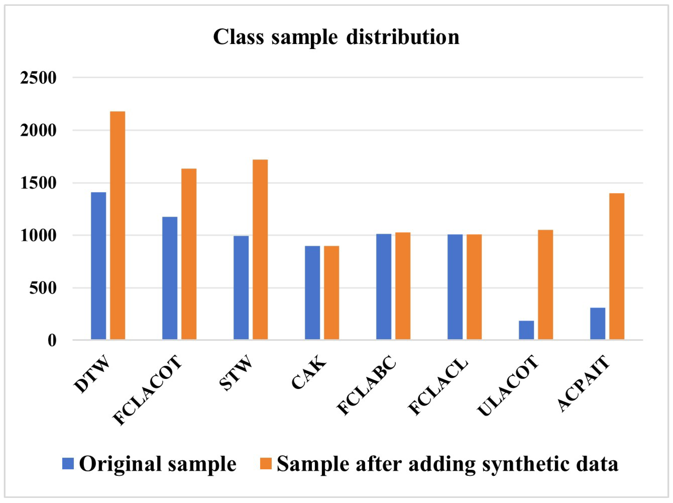
4.2. RCLDs Dataset Supplement
4.2.1. Synthetic Images
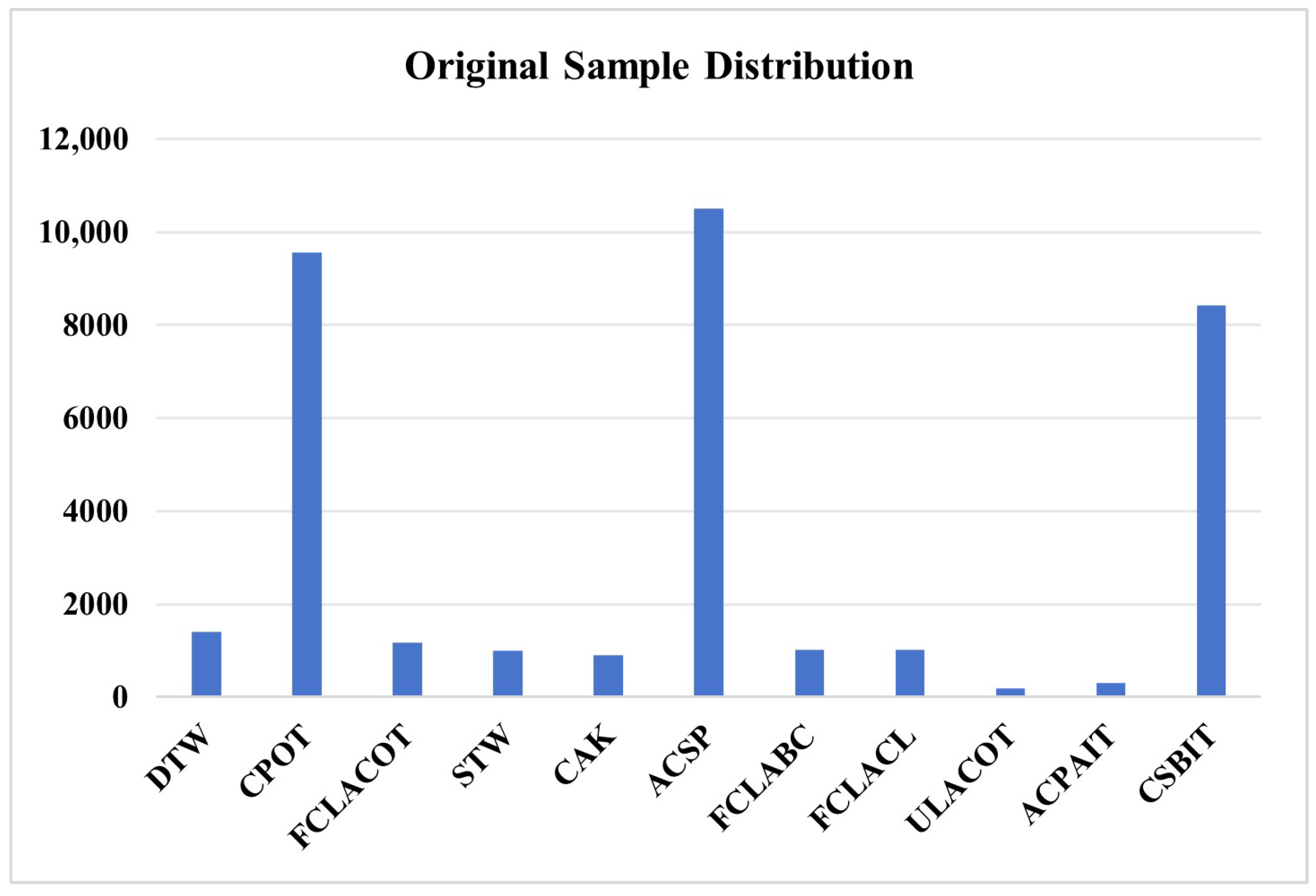
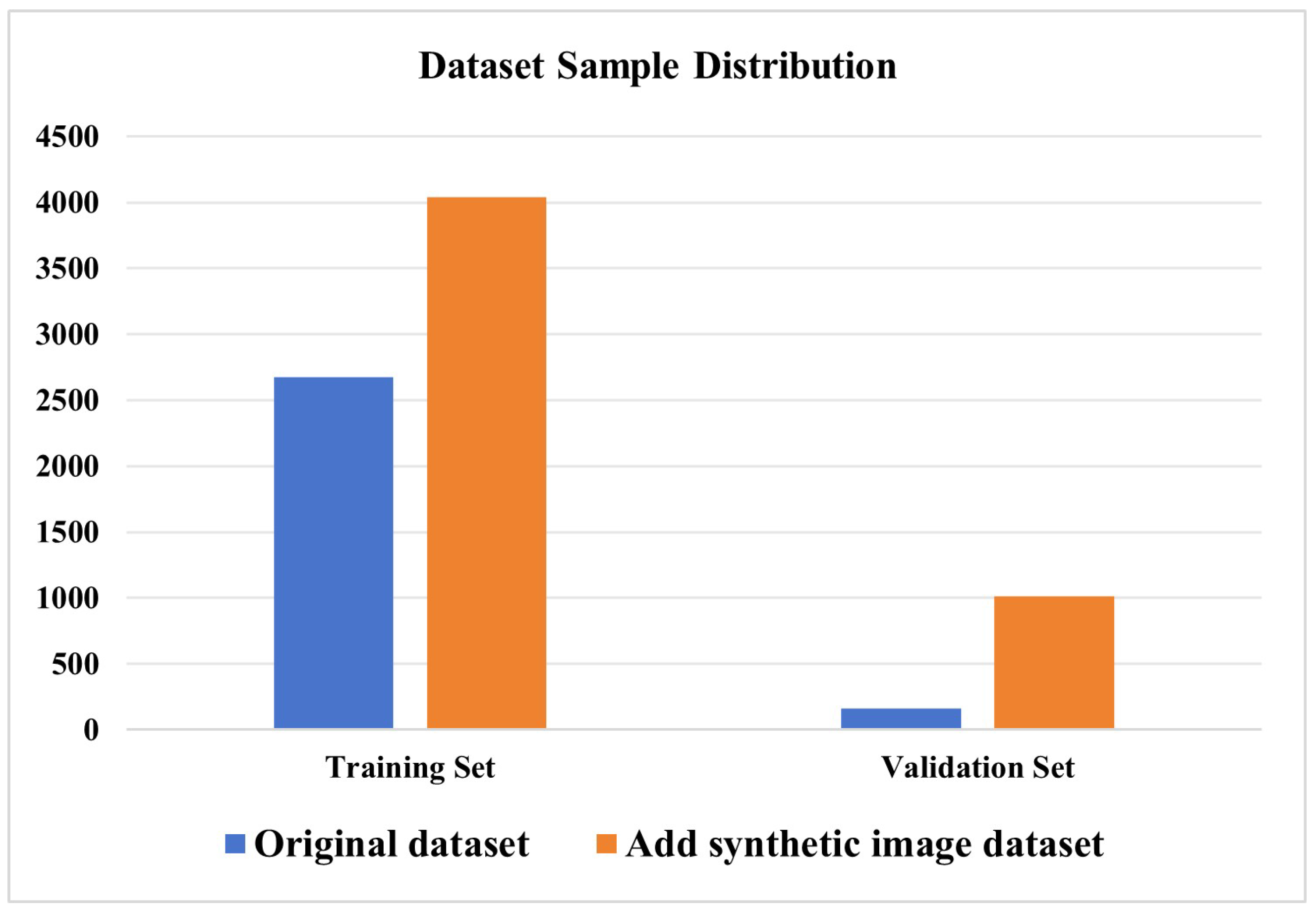
4.2.2. Distribution of RCLDs Dataset
4.3. Analysis of Experimental Results After Adding Synthetic Images
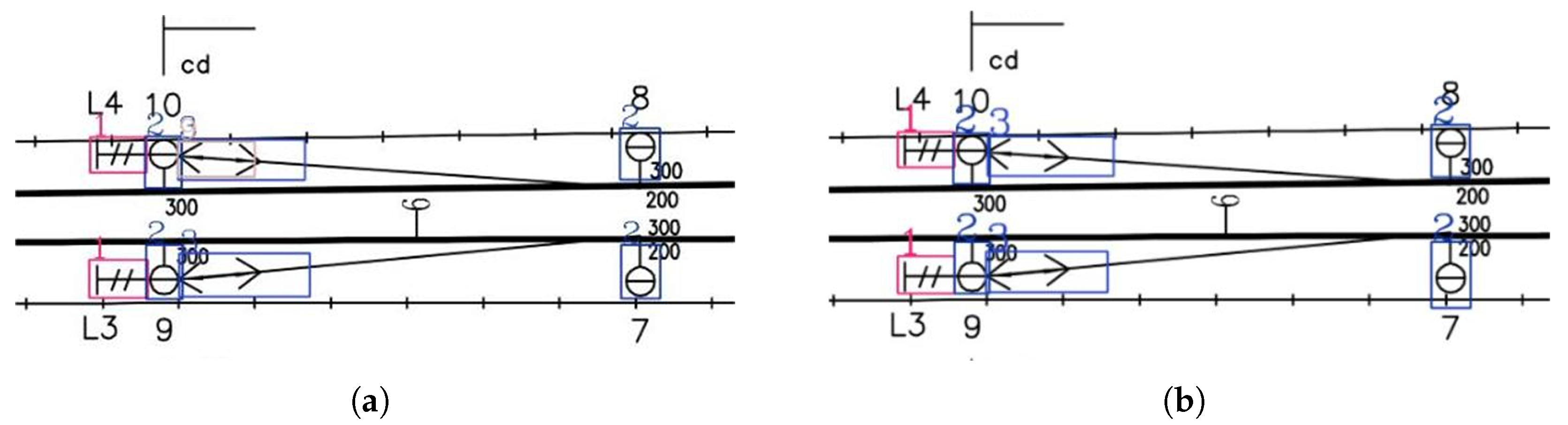
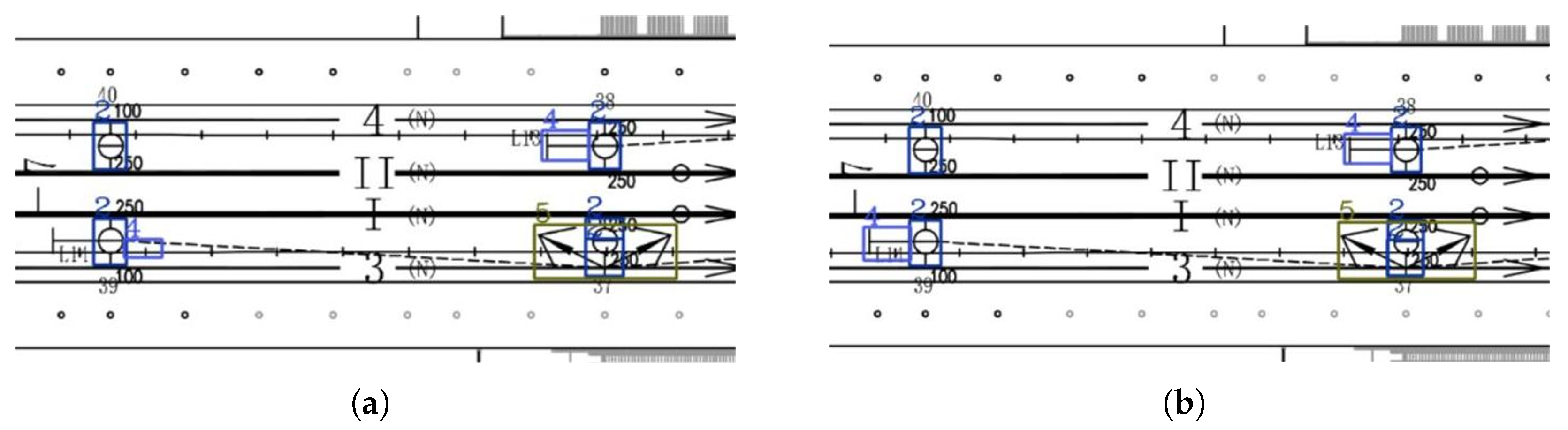
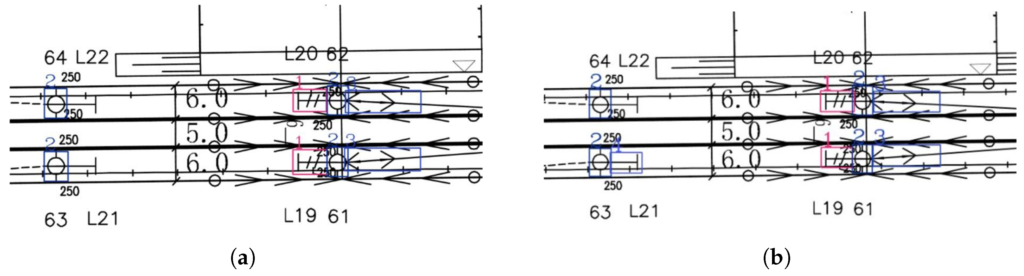
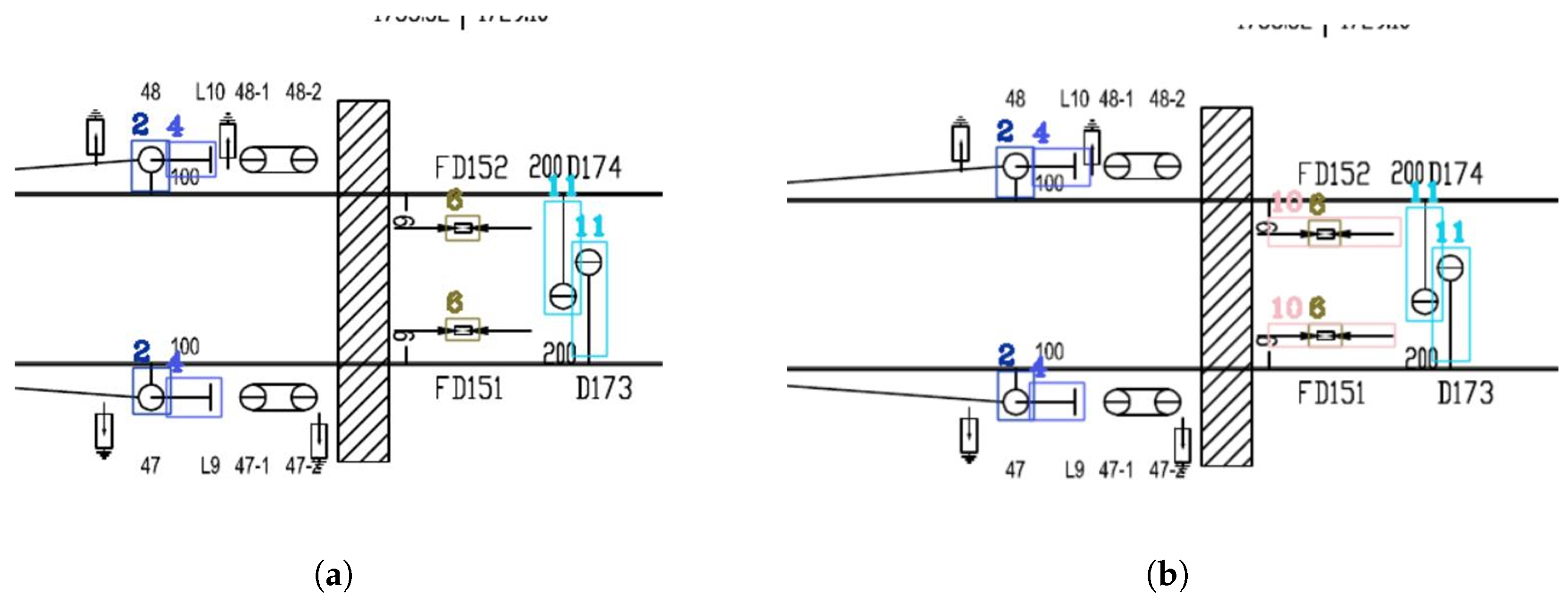
Visualization of Experimental Results
5. Conclusions
Author Contributions
Funding
Data Availability Statement
Conflicts of Interest
References
- Feng, D.; Yu, Q.; Sun, X.; Zhu, H.; Lin, S.; Liang, J. Risk assessment for electrified railway catenary system under comprehensive influence of geographical and meteorological factors. IEEE Trans. Transp. Electrif. 2021, 7, 3137–3148. [Google Scholar] [CrossRef]
- Paliwal, S.; Jain, A.; Sharma, M.; Vig, L. Digitize-PID: Automatic digitization of piping and instrumentation diagrams. In Proceedings of the Trends and Applications in Knowledge Discovery and Data Mining: PAKDD 2021 Workshops, WSPA, MLMEIN, SDPRA, DARAI, and AI4EPT, Delhi, India, 11 May 2021; pp. 168–180. [Google Scholar]
- Paliwal, S.; Sharma, M.; Vig, L. OSSR-PID: One-shot symbol recognition in P&ID sheets using path sampling and GCN. In Proceedings of the 2021 International Joint Conference on Neural Networks (IJCNN), Shenzhen, China, 18–22 July 2021; pp. 1–8. [Google Scholar]
- Okazaki, A.; Kondo, T.; Mori, K.; Tsunekawa, S.; Kawamoto, E. An automatic circuit diagram reader with loop-structure-based symbol recognition. IEEE Trans. Pattern Anal. Mach. Intell. 1988, 10, 331–341. [Google Scholar] [CrossRef]
- Ablameyko, S.V.; Uchida, S. Recognition of engineering drawing entities: Review of approaches. Int. J. Image Graph. 2007, 7, 709–733. [Google Scholar] [CrossRef]
- Kang, S.O.; Lee, E.B.; Baek, H.K. A digitization and conversion tool for imaged drawings to intelligent piping and instrumentation diagrams (P&ID). Energies 2019, 12, 2593. [Google Scholar] [CrossRef]
- Nurminen, J.K.; Rainio, K.; Numminen, J.P.; Syrjänen, T.; Paganus, N.; Honkoila, K. Object detection in design diagrams with machine learning. In Proceedings of the 11th International Conference on Computer Recognition Systems (CORES 2019), Polanica Zdroj, Poland, 20–22 May 2020; pp. 27–36. [Google Scholar]
- Manakitsa, N.; Maraslidis, G.S.; Moysis, L.; Fragulis, G.F. A review of machine learning and deep learning for object detection, semantic segmentation, and human action recognition in machine and robotic vision. Technologies 2024, 12, 15. [Google Scholar] [CrossRef]
- Moreno-García, C.F.; Elyan, E.; Jayne, C. New trends on digitisation of complex engineering drawings. Neural Comput. Appl. 2019, 31, 1695–1712. [Google Scholar] [CrossRef]
- Li, P.; Xue, R.; Shao, S.; Zhu, Y.; Liu, Y. Current state and predicted technological trends in global railway intelligent digital transformation. Railw. Sci. 2023, 2, 397–412. [Google Scholar] [CrossRef]
- Nguyen, M.T.; Pham, V.L.; Nguyen, C.C.; Nguyen, V.V. Object Detection and Text Recognition in Large-Scale Technical Drawings. 2021. Available online: https://eprints.uet.vnu.edu.vn/eprints/id/eprint/4603/ (accessed on 15 August 2021).
- Faltin, B.; Schönfelder, P.; König, M. Inferring interconnections of construction drawings for bridges using deep learning-based methods. In ECPPM 2022-eWork and eBusiness in Architecture, Engineering and Construction 2022; CRC Press: Boca Raton, FL, USA, 2023; pp. 343–350. [Google Scholar]
- Francois, M.; Eglin, V.; Biou, M. Text detection and post-OCR correction in engineering documents. In Proceedings of the International Workshop on Document Analysis Systems, La Rochelle, France, 22–25 May 2022; pp. 726–740. [Google Scholar]
- Sarkar, S.; Pandey, P.; Kar, S. Automatic detection and classification of symbols in engineering drawings. arXiv 2022, arXiv:2204.13277. [Google Scholar]
- Scheibel, B.; Mangler, J.; Rinderle-Ma, S. Extraction of dimension requirements from engineering drawings for supporting quality control in production processes. Comput. Ind. 2021, 129, 103442. [Google Scholar] [CrossRef]
- Jamieson, L.; Francisco Moreno-García, C.; Elyan, E. A review of deep learning methods for digitisation of complex documents and engineering diagrams. Artif. Intell. Rev. 2024, 57, 136. [Google Scholar] [CrossRef]
- Ren, S.; He, K.; Girshick, R.; Sun, J. Faster R-CNN: Towards real-time object detection with region proposal networks. IEEE Trans. Pattern Anal. Mach. Intell. 2016, 39, 1137–1149. [Google Scholar] [CrossRef] [PubMed]
- He, K.; Gkioxari, G.; Dollár, P.; Girshick, R. Mask r-cnn. In Proceedings of the IEEE International Conference on Computer Vision, Venice, Italy, 22–29 October 2017; pp. 2961–2969. [Google Scholar]
- Redmon, J. You only look once: Unified, real-time object detection. In Proceedings of the IEEE Conference on Computer Vision and Pattern Recognition, Las Vegas, NV, USA, 27–30 June 2016. [Google Scholar]
- Liu, W.; Anguelov, D.; Erhan, D.; Szegedy, C.; Reed, S.; Fu, C.Y.; Berg, A.C. Ssd: Single shot multibox detector. In Proceedings of the Computer Vision—ECCV 2016: 14th European Conference, Amsterdam, The Netherlands, 11–14 October 2016; pp. 21–37. [Google Scholar]
- Carion, N.; Massa, F.; Synnaeve, G.; Usunier, N.; Kirillov, A.; Zagoruyko, S. End-to-end object detection with transformers. In Proceedings of the European Conference on Computer Vision, Glasgow, UK, 23–28 August 2020; pp. 213–229. [Google Scholar]
- Bochkovskiy, A.; Wang, C.Y.; Liao, H.Y.M. Yolov4: Optimal speed and accuracy of object detection. arXiv 2020, arXiv:2004.10934. [Google Scholar]
- Ji, S.J.; Ling, Q.H.; Han, F. An improved algorithm for small object detection based on YOLO v4 and multi-scale contextual information. Comput. Electr. Eng. 2023, 105, 108490. [Google Scholar] [CrossRef]
- Ultralytics. YOLOv8. 2023. Available online: https://github.com/ultralytics/ultralytics (accessed on 1 November 2024).
- Wang, Z.; Liu, Y.; Duan, S.; Pan, H. An efficient detection of non-standard miner behavior using improved YOLOv8. Comput. Electr. Eng. 2023, 112, 109021. [Google Scholar] [CrossRef]
- Hao, S.; Li, X.; Peng, W.; Fan, Z.; Ji, Z.; Ganchev, I. YOLO-CXR: A novel detection network for locating multiple small lesions in chest X-ray images. IEEE Access 2024, 12, 156003–156019. [Google Scholar] [CrossRef]
- Tan, W.C.; Chen, I.M.; Tan, H.K. Automated identification of components in raster piping and instrumentation diagram with minimal pre-processing. In Proceedings of the 2016 IEEE International Conference on Automation Science and Engineering (CASE), Fort Worth, TX, USA, 21–24 August 2016; pp. 1301–1306. [Google Scholar]
- Moreno-García, C.F.; Elyan, E.; Jayne, C. Heuristics-based detection to improve text/graphics segmentation in complex engineering drawings. In Proceedings of the Engineering Applications of Neural Networks: 18th International Conference, EANN 2017, Athens, Greece, 25–27 August 2017; pp. 87–98. [Google Scholar]
- Moon, Y.; Lee, J.; Mun, D.; Lim, S. Deep learning-based method to recognize line objects and flow arrows from image-format piping and instrumentation diagrams for digitization. Appl. Sci. 2021, 11, 10054. [Google Scholar] [CrossRef]
- Bhanbhro, H.; Hooi, Y.K.; Kusakunniran, W.; Amur, Z.H. Symbol Detection in a Multi-class Dataset Based on Single Line Diagrams using Deep Learning Models. Int. J. Adv. Comput. Sci. Appl. 2023, 14, 8. [Google Scholar] [CrossRef]
- Su, G.; Zhao, S.; Li, T.; Liu, S.; Li, Y.; Zhao, G.; Li, Z. Image format pipeline and instrument diagram recognition method based on deep learning. Biomim. Intell. Robot. 2024, 4, 100142. [Google Scholar] [CrossRef]
- Yang, L.; Wang, J.; Zhang, J.; Li, H.; Wang, K.; Yang, C.; Shi, D. Practical single-line diagram recognition based on digital image processing and deep vision models. Expert Syst. Appl. 2024, 238, 122389. [Google Scholar] [CrossRef]
- Yazed, M.S.M.; Shaubari, E.F.A.; Yap, M.H. A Review of Neural Network Approach on Engineering Drawing Recognition and Future Directions. JOIV Int. J. Inform. Vis. 2023, 7, 2513–2522. [Google Scholar]
- Elyan, E.; Jamieson, L.; Ali-Gombe, A. Deep learning for symbols detection and classification in engineering drawings. Neural Netw. 2020, 129, 91–102. [Google Scholar] [CrossRef] [PubMed]
- Bhanbhro, H.; Kwang Hooi, Y.; Kusakunniran, W.; Amur, Z.H. A Symbol Recognition System for Single-Line Diagrams Developed Using a Deep-Learning Approach. Appl. Sci. 2023, 13, 8816. [Google Scholar] [CrossRef]
- Frolov, S.; Hinz, T.; Raue, F.; Hees, J.; Dengel, A. Adversarial text-to-image synthesis: A review. Neural Netw. 2021, 144, 187–209. [Google Scholar] [CrossRef] [PubMed]
- Moser, B.; Shanbhag, A.; Raue, F.; Frolov, S.; Palacio, S.; Dengel, A. Diffusion models in image super-resolution and everything: A survey. arXiv 2024, arXiv:2401.00736. [Google Scholar] [CrossRef]
- Croitoru, F.A.; Hondru, V.; Ionescu, R.T.; Shah, M. Diffusion models in vision: A survey. IEEE Trans. Pattern Anal. Mach. Intell. 2023, 45, 10850–10869. [Google Scholar] [CrossRef]
- Bhunia, A.K.; Khan, S.; Cholakkal, H.; Anwer, R.M.; Laaksonen, J.; Shah, M.; Khan, F.S. Person image synthesis via denoising diffusion model. In Proceedings of the IEEE/CVF Conference on Computer Vision and Pattern Recognition, Vancouver, BC, Canada, 17–24 June 2023; pp. 5968–5976. [Google Scholar]
- Wu, Z.; Chen, X.; Xie, S.; Shen, J.; Zeng, Y. Super-resolution of brain MRI images based on denoising diffusion probabilistic model. Biomed. Signal Process. Control 2023, 85, 104901. [Google Scholar] [CrossRef]
- Jiao, J.; Tang, Y.M.; Lin, K.Y.; Gao, Y.; Ma, A.J.; Wang, Y.; Zheng, W.S. Dilateformer: Multi-scale dilated transformer for visual recognition. IEEE Trans. Multimed. 2023, 25, 8906–8919. [Google Scholar] [CrossRef]
- Zhang, X.; Liu, C.; Yang, D.; Song, T.; Ye, Y.; Li, K.; Song, Y. RFAConv: Innovating spatial attention and standard convolutional operation. arXiv 2023, arXiv:2304.03198. [Google Scholar]
- Liu, W.; Lu, H.; Fu, H.; Cao, Z. Learning to upsample by learning to sample. In Proceedings of the IEEE/CVF International Conference on Computer Vision, Paris, France, 1–6 October 2023; pp. 6027–6037. [Google Scholar]
- Sohl-Dickstein, J.; Weiss, E.; Maheswaranathan, N.; Ganguli, S. Deep unsupervised learning using nonequilibrium thermodynamics. In Proceedings of the International Conference on Machine Learning, PMLR, Lille, France, 6–11 July 2015; pp. 2256–2265. [Google Scholar]
- Ho, J.; Jain, A.; Abbeel, P. Denoising diffusion probabilistic models. Adv. Neural Inf. Process. Syst. 2020, 33, 6840–6851. [Google Scholar]
- Nichol, A.Q.; Dhariwal, P. Improved denoising diffusion probabilistic models. In Proceedings of the International Conference on Machine Learning, PMLR, Virtual, 18–24 July 2021; pp. 8162–8171. [Google Scholar]
- Li, C.; Li, L.; Jiang, H.; Weng, K.; Geng, Y.; Li, L.; Ke, Z.; Li, Q.; Cheng, M.; Nie, W.; et al. YOLOv6: A single-stage object detection framework for industrial applications. arXiv 2022, arXiv:2209.02976. [Google Scholar]
- Wang, A.; Chen, H.; Liu, L.; Chen, K.; Lin, Z.; Han, J.; Ding, G. Yolov10: Real-time end-to-end object detection. Adv. Neural Inf. Process. Syst. 2024, 37, 107984–108011. [Google Scholar]


| Group | Original Images | Synthetic Images |
|---|---|---|
| 1 | ✓ | |
| 2 | ✓ | ✓ |
| Method | F1-Score (%) | mAP@0.5 (%) | mAP@0.5:0.95 (%) |
|---|---|---|---|
| Faster R-CNN [17] | 29.5 | 31.4 | — |
| YOLOv4 [22] | 74.4 | 88.5 | 64.3 |
| YOLOv5n | 90.2 | 88.7 | 60.8 |
| YOLOv5s | 91.6 | 88.9 | 64.2 |
| YOLOv6n [47] | 91.4 | 91.3 | 64.3 |
| YOLOv8n [24] | 90.7 | 92.8 | 66.6 |
| YOLOv10n [48] | 90.5 | 92.8 | 67.8 |
| Ours | 93.6 | 94.7 | 68.3 |
| Method | C2f-MSDA | Detect-RFA | DySample | F1 (%) | mAP@0.5 (%) | mAP@0.5:0.95 (%) | Parameter (M) | GFLOPs (G) | FPS |
|---|---|---|---|---|---|---|---|---|---|
| 1 | 90.7 | 92.8 | 66.6 | 3.008 | 8.1 | 175.6 | |||
| 2 | ✓ | 90.7 | 92.7 | 68.3 | 2.752 | 7.6 | 71.5 | ||
| 3 | ✓ | 92.6 | 93.8 | 68.2 | 3.146 | 8.7 | 38.9 | ||
| 4 | ✓ | 91.7 | 93.8 | 67.2 | 3.020 | 8.2 | 154.4 | ||
| 5 | ✓ | ✓ | 92.8 | 93.7 | 67.9 | 2.890 | 8.2 | 28.1 | |
| 6 | ✓ | ✓ | 91.3 | 93.9 | 67.1 | 2.764 | 7.6 | 67.3 | |
| 7 | ✓ | ✓ | 91.9 | 93.5 | 68.9 | 3.159 | 8.8 | 35.4 | |
| 8 | ✓ | ✓ | ✓ | 93.6 | 94.7 | 68.3 | 2.903 | 8.2 | 28.0 |
| Data Source | FID ↓ | IS ↑ | SSIM ↑ | PSNR ↑ | LPIPS ↓ |
|---|---|---|---|---|---|
| IDDPM (Ours) | 55.7077 | 3.2188 | 0.8843 | 29.06 | 0.1995 |
| Symbol | Samples | Original Dataset | Samples | After Adding Synthesized Images | ||||
|---|---|---|---|---|---|---|---|---|
| F1 (%) | mAP@0.5 (%) | mAP@0.5:0.95 (%) | F1 (%) | mAP@0.5 (%) | mAP@0.5:0.95 (%) | |||
| DTW | 93 | 95.3 | 95.3 | 69.5 | 452 | 96.7 | 97.7 | 84.5 |
| CPOT | 557 | 96.1 | 97.7 | 72.4 | 2268 | 95.9 | 97.7 | 85.3 |
| FCLACOT | 82 | 98.1 | 98.7 | 68.3 | 325 | 97.1 | 97.8 | 82.1 |
| STW | 55 | 87.8 | 92.8 | 65.4 | 352 | 98.4 | 99.3 | 85.4 |
| CAK | 45 | 96.4 | 99.2 | 77.4 | 156 | 96.6 | 96.7 | 83.5 |
| ACSP | 402 | 99.3 | 99.5 | 76.6 | 2001 | 98.6 | 99.3 | 77.2 |
| FCLABC | 33 | 99.1 | 99.5 | 76.5 | 165 | 97.7 | 98.5 | 81.2 |
| FCLACL | 34 | 96.8 | 97.9 | 71.8 | 161 | 97.7 | 99.3 | 72.4 |
| ULACOT | 9 | 95.3 | 99.5 | 53.7 | 245 | 95.1 | 97.7 | 82.1 |
| ACPAIT | 6 | 65.4 | 62.1 | 31.6 | 248 | 99.5 | 99.5 | 82.8 |
| CSBIT | 349 | 99.5 | 99.5 | 88 | 1507 | 99.5 | 99.5 | 88.5 |
| TOTAL | 1665 | 93.6 | 94.7 | 68.3 | 7880 | 97.6 | 98.5 | 82.3 |
Disclaimer/Publisher’s Note: The statements, opinions and data contained in all publications are solely those of the individual author(s) and contributor(s) and not of MDPI and/or the editor(s). MDPI and/or the editor(s) disclaim responsibility for any injury to people or property resulting from any ideas, methods, instructions or products referred to in the content. |
© 2025 by the authors. Licensee MDPI, Basel, Switzerland. This article is an open access article distributed under the terms and conditions of the Creative Commons Attribution (CC BY) license (https://creativecommons.org/licenses/by/4.0/).
Share and Cite
Sun, Q.; Zhu, M.; Li, M.; Li, G.; Deng, W. Symbol Recognition Method for Railway Catenary Layout Drawings Based on Deep Learning. Symmetry 2025, 17, 674. https://doi.org/10.3390/sym17050674
Sun Q, Zhu M, Li M, Li G, Deng W. Symbol Recognition Method for Railway Catenary Layout Drawings Based on Deep Learning. Symmetry. 2025; 17(5):674. https://doi.org/10.3390/sym17050674
Chicago/Turabian StyleSun, Qi, Mengxin Zhu, Minzhi Li, Gaoju Li, and Weizhi Deng. 2025. "Symbol Recognition Method for Railway Catenary Layout Drawings Based on Deep Learning" Symmetry 17, no. 5: 674. https://doi.org/10.3390/sym17050674
APA StyleSun, Q., Zhu, M., Li, M., Li, G., & Deng, W. (2025). Symbol Recognition Method for Railway Catenary Layout Drawings Based on Deep Learning. Symmetry, 17(5), 674. https://doi.org/10.3390/sym17050674