Probabilistic Analysis of Distributed Fractional-Order Stochastic Systems Driven by Fractional Brownian Motion: Existence, Uniqueness, and Transportation Inequalities

Abstract

This paper investigates a class of distributed fractional-order stochastic differential equations driven by fractional Brownian motion with a Hurst parameter $1/2<H<1$. By employing the Picard iteration method, we rigorously prove the existence and uniqueness of solutions with Lipschitz conditions. Furthermore, leveraging the Girsanov transformation argument within the $L^2$ metric framework, we derive quadratic transportation inequalities for the law of the strong solution to the considered equations. These results provide a deeper understanding of the regularity and probabilistic properties of the solutions in this framework.

1. Introduction

In the past decade, stochastic differential equations have significantly attracted the attention of many researchers due to their wide applications in economics, biology, computing, engineering and chemistry (see [1,2,3,4]). The fractional derivative of a constant is not equal to zero, unlike the classical derivative. It is evident that, within the domain of fractional derivatives, the Riemann–Liouville fractional derivative is the most prevalent and significant. Almost all other definitions of fractional derivatives are available as the special cases of Riemann–Liouville fractional derivatives. The development of theoretical frameworks and their subsequent practical applications have resulted in a marked increase in interest in all aspects of fractional (stochastic) differential equations (see, e.g., [5,6,7,8,9]). A constant-order fractional differential equation is unable to adequately reflect the inherent uncertainty present in the data, thus necessitating the introduction of variable-order operators to accommodate the structural changes occurring in the surrounding context. Numerous significant results have been obtained pertaining to both variable-order fractional derivatives and variable-order (stochastic) fractional differential equations, for which we can refer to [10,11,12,13,14]. Furthermore, a distributed-order fractional derivative is defined by

$${}_{0}D_t^{\rho }u(x,t):={\int }_0^1\rho \left(\theta \right){\partial }_t^{\theta }u(x,t)d\theta$$

(1)

where $\rho =\rho \left(\theta \right)$ is a probability density function (see [10]). The objective is to provide a framework for creating data-driven fractional differential operators that can be used to fit data directly from real measurements. This will result in a more effective model of uncertainties [15,16]. ${\partial }_t^{\alpha }$ is the Riemann–Liouville fractional differential operator defined by

$$\begin{array}{cc}\hfill {\partial }_t^{\alpha }g\left(t\right)& :={\displaystyle \frac{d}{dt}}\left[{}_{0}J_t^{1-\alpha }g\left(t\right)\right],\hfill \\ \hfill {}_{0}J_t^{1-\alpha }g\left(t\right)& :={\displaystyle \frac{1}{\Gamma (1-\alpha )}}{\int }_0^t{\displaystyle \frac{g\left(s\right)ds}{{(t-s)}^{\alpha }}},\alpha \in (0,1).\hfill \end{array}$$

(2)

Over the past few years, there has been a marked increase in the interest surrounding the study of fractional Brownian motion and associated processes. This trend has been driven by their applications in diverse fields, including finance, telecommunications, image processing, and turbulence. A fractional Brownian motion of Hurst parameter $H\in (0,1)$ is a centered Gaussian process $B^H=\{B^H\left(t\right),t\ge 0\}$ with the covariance function

$$R_H(t,s)=\mathbb{E}\left(B^H\left(t\right)B^H\left(s\right)\right)={\displaystyle \frac{1}{2}}(t^{2H}+s^{2H}{-|t-s|}^{2H}).$$

When $H=1/2$, the fractional Brownian motion (fBm) $B^H$ reduces to standard Brownian motion, whose increments are independent. For $H\ne 1/2$, the process $B^H$ loses both the semimartingale property and Markovianity due to its non-local covariant structure. This behavior has spurred significant research on stochastic differential equations driven by fBm; we refer to [17,18,19,20,21,22,23,24] for comprehensive reviews.

Motivated by the above discussion, the aim of this paper is to present a discussion of the following distributed-order fractional stochastic differential equations driven by fractional Brownian motion:

$$\begin{array}{cc}\hfill dz\left(t\right)& =\left(-\mu {}_{0}D_t^{\rho }z\left(t\right)+a(z\left(t\right)\right)dt+b\left(z\left(t\right)\right)d{B}^H\left(t\right)\hfill \\ \hfill & =d\left({\int }_0^1\rho \left(\alpha \right){\int }_0^t{\displaystyle \frac{-\mu z\left(s\right)}{\Gamma (1-\alpha ){(t-s)}^{\alpha }}}dsd\alpha \right)+a\left(z\left(s\right)\right)dt+b\left(z\left(s\right)\right)d{B}^H\left(t\right),\hfill \end{array}$$

(3)

with initial condition $z\left(0\right)=z_0$. Here, $\mu \ge 0$ is a constant and $B^H\left(t\right)$ is a fractional Brownian motion with Hurst parameter $1/2<H<1$, and $a,b:\mathbb{R}\to \mathbb{R}$ are all progressively measurable with further conditions specified in the sequel. Consequently, the definition of the fractional integral and derivative can be utilized to reformulate

$$z\left(t\right)=z_0+{\int }_0^1\rho \left(\alpha \right){\int }_0^t\kappa (t,s,\alpha )z\left(s\right)dsd\alpha +{\int }_0^{t}a\left(z\left(s\right)\right)ds+{\int }_0^{t}b\left(z\left(s\right)\right)d{B}^H\left(s\right),$$

(4)

where $z\left(t\right)\in R$ is a stochastic process and $z_0$ is $F_0$-measurable. The following definition applies to the kernel $\kappa (t,s,\alpha )$:

$$\kappa (t,s,\alpha ):={\displaystyle \frac{-\mu }{\Gamma (1-\alpha ){(t-s)}^{\alpha }}}.$$

(5)

Our first result (Theorem 1) proves the well-posedness of (4) through a fractional Picard scheme, extending classical techniques to the distributed-order case.

Meanwhile, transportation inequality (TCI) provides an error analysis and an optimization basis for engineering problems such as physical simulation, signal processing, and material design by quantifying differences among probability distributions. Its core value is to transform the statistical behavior of complex systems into computable distributed matching problems, thus guiding algorithm improvement and practical application. TCIs for stochastic processes have attracted growing interest, owing to their connections with Tsirelson-type inequalities, Hoeffding-type inequalities [25,26,27], and the concentration of empirical measures [28,29]. The Girsanov transformation argument is one of the most effective methods for establishing transportation inequality [25]. Most of the results concerning the TCI of stochastic processes are derived thanks to the Girsanov transformation argument. For instance, as outlined in [26,27], the study focuses on diffusion processes on ${\mathbb{R}}^d$, while [30] examines multidimensional semimartingales. The literature further extends to SDEs with pure jump processes, as detailed in [29], and [31] for SDEs driven by a fractional Brownian motion, [32] for stochastic delay evolution equations driven by fBm with Hurst parameter $H\in (1/2,1)$, and [33] for neutral stochastic evolution equations driven by fBm with Hurst parameter $H\in (0,1/2)$.

Now, our analysis focuses on the following inequalities. The discrepancy between probability measures is assessed via the transportation metric, formally defined as the Wasserstein distance. Let $(E,d)$ be a metric space equipped with a $\sigma$-field B such that the distance d is $B\otimes B$-measurable. Given $p⩾1$ and two probability measures $\mu$ and $\nu$ on E, the Wasserstein distance is defined by

$$W_p^d(\mu ,\nu )=\underset{\pi \in C(\mu ,\nu )}{inf}{\left(\int \int d{(x,y)}^{p}d\pi (x,y)\right)}^{1/p},$$

where $C(\mu ,\nu )$ denotes the totality of probability measures on $E\times E$ with the marginal $\mu$ and $\nu .$ The relative entropy of $\nu$ with respect to $\mu$ is defined as

$$\mathbf{H}(\nu \mid \mu )=\left\{\begin{array}{cc}\int log{\displaystyle \frac{d\nu }{d\mu }}d\nu ,\hfill & \nu \ll \mu ,\hfill \\ +\infty ,\hfill & \mathrm{otherwise}.\hfill \end{array}\right.$$

As is customary, the relation is written as $\mu \in T_p\left(C\right)$ for this particular instance. The cases $p=1$ and $p=2$ have been most extensively studied. The distinctive properties of $T_2\left(C\right)$ hold significant theoretical importance. Therefore, the second objective of this work is to derive transport inequalities (TCIs) for the solution law of Equation (4) in the $L^2$ metric via Girsanov transformation.

The framework of this paper is as follows: In Section 2, the fractional Brownian properties of fractional Brownian are presented, along with the assumptions and auxiliary results that are employed to substantiate the mathematical estimates in subsequent sections. In Section 3, we complete the demonstration of existence and uniqueness of the solution to the equation. In Section 4, we prove $T_2\left(C\right)$ of Equation (4) under the $L^2$ metric.

2. Preliminaries

This section is dedicated to the collection of relevant notions, conceptions and lemmas pertaining to Wiener integral with respect to fractional Brownian motion. For further information, we refer to [34,35,36]. And then, we make some assumptions for the model. In this paper, unless explicitly indicated otherwise, we consider the complete probability space $(\Omega ,\mathcal{F},{\left\{{\mathcal{F}}_t\right\}}_{t\ge 0},\mathbb{P})$ to be a filtration satisfying the standard conditions, namely that it is right-continuous and that ${\mathcal{F}}_0$ contains all $\mathbb{P}$ empty sets. The symbol $\mathbb{E}$ denotes the expectation under the probability measure $\mathbb{P}$. Stochastic processes are specified on the set $(\Omega ,\mathcal{F},{\left\{{\mathcal{F}}_t\right\}}_{t\ge 0},\mathbb{P})$. If $z\in \mathbb{R}$, then $\left|z\right|$ is the absolute value. The symbol K is employed to denote any constant, the value of which is of no consequence and is subject to variation from one line of argument to another.

2.1. Fractional Brownian Motion and Wick Product

Consider a finite time horizon $T>0$ and let ${\left\{B_t^H\right\}}_{t\ge 0}$ denote a one-dimensional fractional Brownian motion (fBm) with Hurst parameter $H\in (1/2,1)$. It should be acknowledged that, in the event that $H\in (1/2,1)$, the Wiener integral representation of ${\left\{B_t^H\right\}}_{t\ge 0}$ is given by the following expression:

$$B_t^H={\int }_0^t{K}^H(t,s)d{W}_s,$$

where ${\left\{W_t\right\}}_t\ge 0$ is a Wiener process. The kernel function $K^H(t,s)$ is given by

$$K_H(t,s)=c_H{s}^{{\displaystyle \frac{1}{2}}-H}{\int }_0^t{(u-s)}^{H-{\displaystyle \frac{3}{2}}}{u}^{H-{\displaystyle \frac{1}{2}}}du,$$

and $c_H={\left({\displaystyle \frac{H(2H-1)}{B(2-2H,H-\frac{1}{2})}}\right)}^{{\displaystyle \frac{1}{2}}}$, in which $B(·,·)$ is the Beta function, and $t>s$. For a more comprehensive overview of the fractional Brownian motion (fBm), the reader is referred to the following works [34,37,38].

Let $\mathcal{I}$ denote the set of all finite multi-indices $\alpha =({\alpha }_1,\cdots ,{\alpha }_n)$, where ${\alpha }_n$ are non-negative integers for all $n\ge 1$. Denote $\left|\alpha \right|={\alpha }_1+\cdots +{\alpha }_n$, and $\alpha !={\alpha }_1!\cdots {\alpha }_n!$. For $n\ge 0$, the Hermite polynomials are defined as follows:

$$h_n\left(x\right)={(-1)}^n{e}^{x^2}{\displaystyle \frac{d^n}{d{x}^n}}\left(e^{-x^2}\right),$$

and Hermite functions

$${\tilde{h}}_n\left(x\right)={\pi }^{-{\displaystyle \frac{1}{4}}}{(n!)}^{-{\displaystyle \frac{1}{2}}}{h}_n\left(x\right)e^{-{\displaystyle \frac{x^2}{4}}}.$$

Let $S\left(\mathbb{R}\right)$ be the Schwartz space of rapidly decreasing infinitely differentiable real-valued functions and let $S^{\prime }\left(\mathbb{R}\right)$ be the dual space of $S\left(\mathbb{R}\right)$. Setting

$${\mathcal{H}}_{\alpha }\left(\omega \right)=\prod _{i=1}^n{h}_{{\alpha }_i}\left(⟨{\tilde{h}}_i\left(x\right),\omega ⟩\right),$$

to be the product of Hermite polynomials. Consider a square-integrable random variable

$$F=F\left(\omega \right)\in L^2(S^{\prime }\left(\mathbb{R}\right),\mathcal{F},P).$$

Thus, following [34,39], every $F\left(\omega \right)$ admits a unique representation

$$F\left(\omega \right)=\sum _{\alpha \in \mathcal{I}}{c}_{\alpha }{\mathcal{H}}_{\alpha }\left(\omega \right),$$

and

$${\parallel F\parallel }_{L^2\left(\omega \right)}^2=\sum _{\alpha \in \mathcal{I}}{c}_{\alpha }!c_{\alpha }^2<\infty .$$

where $F\left(\omega \right)={\sum }_{\alpha \in \mathcal{I}}{c}_{\alpha }{\mathcal{H}}_{\alpha }\left(\omega \right)$ and $G\left(\omega \right)={\sum }_{\beta \in \mathcal{I}}{d}_{\beta }{\mathcal{H}}_{\beta }\left(\omega \right)$. Their Wick product [36] is defined by

$$F\diamond G\left(\omega \right)=\sum _{\alpha ,\beta \in \mathcal{I}}{a}_{\alpha }{b}_{\beta }{\mathcal{H}}_{\alpha +\beta }\left(\omega \right)=\sum _{\gamma \in \mathcal{I}}\left(\sum _{\alpha +\beta =\gamma }{a}_{\alpha }{b}_{\beta }\right){\mathcal{H}}_{\gamma }\left(\omega \right).$$

2.2. Malliavin Derivative

Let $p\ge 1,L^p:=L^p(\Omega ,\mathcal{F},\mathbb{P})$ be the space of all random variables $\Omega \to \mathbb{R}$, such that

$${\parallel F\parallel }_p={\mathbb{E}\left(\right|F|}^p{)}^{1/p}<\infty ,$$

and let

$$L_{\varphi }^2\left({\mathbb{R}}_{+}\right)=\left\{\right|f:{\mathbb{R}}_{+}\to {\mathbb{R},\left|f\right|}_{\varphi }^2:={\int }_0^{\infty }{\int }_0^{\infty }f\left(s\right)f\left(t\right)\varphi (s,t)dsdt<\infty \},$$

where $\varphi (s,t)={H(2H-1)|s-t|}^{2H-2}.$

Let $g\in L_{\varphi }^2\left(\mathbb{R}\right)$. The $\varphi$-derivative of a stochastic variable $F\in L^p$ in the direction of ${\Phi }_g$ is defined by

$$D_{{\Phi }_g}F\left(\omega \right)=\underset{\delta \to 0}{lim}{\displaystyle \frac{1}{\delta }}\left\{F(\omega +\delta {\int }_0^{·}\left({\Phi }_g\right)\left(u\right)du)-F\left(\omega \right)\right\},$$

if the limit exists in $L^p$. Moreover, if there exists a process $D_s^{\varphi }{F}_s$, $s\ge 0$ such that

$$D_{{\Phi }_g}F={\int }_0^{\infty }{D}_s^{\varphi }{F}_s{g}_{s}dsa.s.,$$

for all $g\in L_{\varphi }^2\left(\mathbb{R}\right)$, then F is said to be $\varphi$-differentiable.

Let $\mathcal{A}[0,T]$ be the family of stochastic processes on $[0,T]$ such that $F\in \mathcal{A}(0,T)$ if ${\mathbb{E}\left|F\right|}_{\varphi }^2<\infty$ and F is $\varphi$-differentiable, the trace of $(D_s^{\varphi }{F}_t,0\le s\le T,0\le t\le T)$ exists and $\mathbb{E}{\int }_0^T{\left(D_s^{\varphi }{F}_s\right)}^{2}ds<\infty$, and for each sequence of partitions ${\pi }_n,n\in {\mathbb{N}}_{+}$ such that ${\pi }_n\to 0$, as $n\to \infty$. Moreover,

$$\sum _{i=0}^{n-1}\mathbb{E}{\left\{{\int }_{t_t^{\left(n\right)}}^{t_{i+1}^{\left(n\right)}}|D_s^{\varphi }{F}_{t_i^{\left(n\right)}}^{\pi }-D_s^{\varphi }{F}_s|ds\right\}}^2\to 0,$$

and

$$\mathbb{E}|F^{\pi }{-F|}_{\varphi }^2\to 0,$$

as $n\to \infty$. Here, ${\pi }_n:0=t_0^{\left(n\right)}<t_1^{\left(n\right)}<\cdots <t_n^{\left(n\right)}=T.$

Next, we define a stochastic integral with respect to fBm.

Let ${\left\{F_t\right\}}_{t\ge 0}$ be a stochastic process such that $F\in \mathcal{A}(0,T)$, then the stochastic integral satisfies $\mathbb{E}{\int }_0^T{F}_{s}d{B}_s^H$ by

$${\int }_0^T{F}_{s}d{B}_s^H=\underset{\left|\pi \right|\to 0}{lim}\sum _{i=0}^{n-1}{F}_{t_i}^{\pi }\diamond (B_{t_{i+1}}^H-B_{t_i}^H),$$

where $\left|\pi \right|=max\{t_{i+1}-t_i,i=0,1\cdots ,n-1\}$.

(I) According to Theorem $3.6.1$ in [36], if $F_s\in \mathcal{A}(0,T)$, then the stochastic integral satisfies $\mathbb{E}{\int }_0^T{F}_{s}d{B}_s^H=0$, and

$$\mathbb{E}{\left|{\int }_0^T{F}_{s}d{B}_s^H\right|}^2=\mathbb{E}\left[{\left({\int }_0^T{D}_s^{\varphi }{F}_{s}ds\right)}^2+{\left|{\mathtt{1}}_{[0,T]}F\right|}_{\varphi }^2\right].$$

By Definition $3.4.1$ in [36], the above stochastic integral can be extended as follows:

$${\int }_{\mathbb{R}}{F}_{t}d{B}_t^H:={\int }_{\mathbb{R}}{F}_t\diamond W^H\left(t\right)dt,$$

where $F:\mathbb{R}\to {\left(\mathcal{S}\right)}_H^{\ast }$ is a given function such that $F_t\diamond W^H\left(t\right)$ is $dt$-integrable in ${\left(\mathcal{S}\right)}_H^{\ast }$. Here, ${\left(\mathcal{S}\right)}_H^{\ast }$ is the fractional Hida distribution space defined by Definition $3.1.11$ in [36]. And in this extension, the integral on an interval $[0,T]$ can be defined by

$${\int }_0^T{F}_{t}d{B}_t^H={\int }_{\mathbb{R}}{F}_t{I}_{[0,T]}\left(t\right)d{B}_t^H.$$

(II) For $H={\displaystyle \frac{1}{2}}$, the definition of stochastic integrals ${\int }_0^T{F}_{s}d{B}_t^H$ and ${\int }_0^{\infty }{F}_{s}d{B}_t^H$ can be found in textbooks (cf., Chapter 3 of the work by Karatzas and Shreve [40]).

According to Remark 1 and Lemma 2 in [41], the following lemma is obtained.

Lemma 1.

Let $B^H\left(t\right)$ be an fBm with Hurst index $H>{\displaystyle \frac{1}{2}}$, and let a stochastic process $\eta \left(t\right)\in {\mathcal{L}}_{\varphi }[0,T]\cap {\mathbb{D}}^{1,2}\left(\right|\mathcal{H}\left|\right).$ Then, for every $T<\infty$,

$$\mathbb{E}{\left[{\int }_0^T\eta \left(u\right)d{B}^H\left(u\right)\right]}^2\le 2H{T}^{2H-1}\mathbb{E}\left[{\int }_0^T|\eta \left(u\right){|}^{2}du\right]+4T\mathbb{E}{\int }_0^T{\left[D_u^{\varphi }\eta \left(u\right)\right]}^{2}du.$$

(6)

Lemma 2

(Discrete Jensen’s inequality). For $r_i\in \mathbb{R}$, we have

$${(r_1+r_2+\cdots +r_m)}^2\le m(r_1^2+r_2^2+\cdots +r_m^2).$$

(7)

Lemma 3

(Borel–Cantelli lemma). Let ${\left\{A_n\right\}}_{n=1}^{\infty }$ be events in a probability such that ${\sum }_{n=1}^{\infty }\mathbb{P}\left(A_n\right)<\infty$, then

$$\mathbb{P}\left(A_{n,m}\right)<\infty ,$$

where $A_{n,m}$ is defined by ${\bigcap }_{n=1}^{\infty }{\bigcup }_{m=n}^{\infty }{A}_m.$

Lemma 4

(Generalized Gronwall inequality). Let $C_0\left(t\right)$ be a non-negative locally integrable function on $[a,b)$ and $C_1$ be a non-negative constant. Suppose $w\left(t\right)$ is a non-negative locally integrable function on $[a,b)$ with

$$w\left(t\right)\le C_0\left(t\right)+C_1{\int }_a^{t}w\left(s\right){(t-s)}^{\beta -1}ds,\forall t\in [a,b),$$

where $0<\beta <1,then$

$$w\left(t\right)\le C_0\left(t\right)+{\int }_a^t\sum _{n=1}^{\infty }{\displaystyle \frac{{\left(C_1\Gamma \left(\beta \right)\right)}^n}{\Gamma \left(n\beta \right)}}{(t-s)}^{n\beta -1}{C}_0\left(s\right)ds,\forall t\in [a,b).$$

In particular, if $C_0\left(t\right)$ is non-decreasing, then

$$w\left(t\right)\le C_0\left(t\right)E_{\beta ,1}\left(C_1\Gamma \left(\beta \right){(t-a)}^{\beta }\right),\forall t\in [a,b),$$

where $E_{p,q}\left(z\right)$ represents the Mittag–Leffler function

$$E_{p,q}\left(z\right):=\sum _{k=0}^{\infty }{\displaystyle \frac{z^k}{\Gamma (pk+q)}},z\in \mathbb{R},p\in {\mathbb{R}}^{+},q\in \mathbb{R}.$$

(8)

In this paper, we proceed with the following assumptions:

• (H1) ${\int }_0^1\rho \left(\alpha \right)d\alpha =1$ and $\rho \left(\alpha \right)\equiv 0$ on $[{\alpha }^{\ast },1]$ for some $0<{\alpha }^{\ast }<1$ and $\mathbb{E}\left[x_0^2\right]<\infty$.
• (H2) There exists $L>0$ such that for $\mathrm{all}y,\tilde{y}\in \mathbb{R}$, $t\in [0,T],$

  $$\begin{array}{cc}& |a\left(z\right)-a\left(\tilde{z}\right){|}^2+|b\left(z\right)-b\left(\tilde{z}\right){|}^2+|D_u^{\varphi }(b\left(z\right)-b\left(\tilde{z}\right)){|}^2\le L{|z-\tilde{z}|}^2.\hfill \end{array}$$
• (H3) There exists $L>0$ such that for all $y\in \mathbb{R}$, $t\in [0,T]$,

  $${\left|a\left(z\right)\right|}^2+{\left|b\left(z\right)\right|}^2+{\left|D_u^{\varphi }b\left(z\right)\right|}^2\le L\left(1+{\left|z\right|}^2\right).$$

3. Existence and Uniqueness

Theorem 1.

Under Assumptions (H1)–(H3), the stochastic differential equation driven by fBm (4) admits a unique solution on the time interval [0,T]:

$$\underset{0\le s\le t}{sup}\mathbb{E}{\left|z\left(s\right)\right|}^2\le Q_0{E}_{1-{\alpha }^{\ast },1}\left(Q_1\Gamma (1-{\alpha }^{\ast })t^{1-{\alpha }^{\ast }}\right),$$

where the constants $Q_0$ and Q₁ are given by

$$Q_0=4\mathbb{E}\left[z_0^2\right]+4LT(5T+2H{T}^{2H-1}),$$

$$Q_1={\displaystyle \frac{4{\mu }^2{Q}_2^{2{\alpha }^{\ast }}{T}^{1-{\alpha }^{\ast }}}{1-{\alpha }^{\ast }}}+4L{T}^{{\alpha }^{\ast }}(5T+2H{T}^{2H-1}).$$

$$Q_2=max\{1,T\}.$$

Proof. 

The existence and uniqueness theorem is demonstrated through the utilization of Picard iteration, a method employed to prove the aforementioned theorem. The following definition is required: a sequence of processes ${\left\{z_n\left(t\right)\right\}}_{n=0}^{\infty }$ by $z_0\left(t\right):=z_0$, and for $n\ge 1$, the following apply. Existence:

(1) 

Structural Picard sequence:

$$z_n\left(t\right):=z_0+{\int }_0^1\rho \left(\alpha \right){\int }_0^t\kappa (t,s,\alpha )z_{n-1}\left(s\right)dsd\alpha +{\int }_0^{t}a\left(z_{n-1}\left(s\right)\right)ds+{\int }_0^{t}b\left(z_{n-1}\left(s\right)\right)d{B}^H\left(t\right).$$

(9)

Then, we observe that

$$\begin{array}{cc}\hfill z_{n+1}\left(t\right)-z_n\left(t\right)& ={\int }_0^1\rho \left(\alpha \right){\int }_0^t\kappa (t,s,\alpha )\left(z_n\left(s\right)-z_{n-1}\left(s\right)\right)dsd\alpha \hfill \\ \hfill & +{\int }_0^t\left(a\left(z_n\left(s\right)\right)-a\left(z_{n-1}\left(s\right)\right)\right)ds\hfill \\ \hfill & +{\int }_0^t\left(b\left(z_n\left(s\right)\right)-b\left(z_{n-1}\left(s\right)\right)\right)d{B}^H\left(s\right).\hfill \end{array}$$

(10)

By using Jensen’s inequality (7) with $m=3$, we obtain

$$\begin{array}{cc}\hfill \mathbb{E}\left[{\left|z_{n+1}\left(t\right)-z_n\left(t\right)\right|}^2\right]& \le 3\mathbb{E}{\left|{\int }_0^1\rho \left(\alpha \right){\int }_0^t\kappa \left(t,s,\alpha \right)\left(z_n\left(s\right)-z_{n-1}\left(s\right)\right)dsd\alpha \right|}^2\hfill \\ \hfill & +3\mathbb{E}{\left|{\int }_0^t\left(a\left(z_n\left(s\right)\right)-a\left(z_{n-1}\left(s\right)\right)\right)ds\right|}^2\hfill \\ \hfill & +3\mathbb{E}{\left|{\int }_0^t\left(b\left(z_n\left(s\right)\right)-b\left(z_{n-1}\left(s\right)\right)\right)d{B}^H\left(s\right)\right|}^2\hfill \\ \hfill & =:G_1+G_2+G_3.\hfill \end{array}$$

(11)

The next step is to establish a constraint on $\kappa (t,s,\alpha )$ in Equation (5)

$$\left|\kappa (t,s,\alpha )\right|=\left|{\displaystyle \frac{-\mu }{\Gamma (1-\alpha ){(t-s)}^{\alpha }}}\right|={\displaystyle \frac{\mu {(t-s)}^{{\alpha }^{\ast }-\alpha }}{\Gamma (1-\alpha ){(t-s)}^{{\alpha }^{\ast }}}},\alpha <{\alpha }^{\ast },$$

if $t-s\le 1$, ${(t-s)}^{{\alpha }^{\ast }-\alpha }\le 1$; if $t-s>1$, ${(t-s)}^{{\alpha }^{\ast }-\alpha }\le T^{{\alpha }^{\ast }-\alpha }\le T^{{\alpha }^{\ast }}.$ Define $Q_2=max\{1,T\}$, ${(t-s)}^{{\alpha }^{\ast }-\alpha }\le Q_2^{{\alpha }^{\ast }}$. So,

$$\left|\kappa (t,s,\alpha )\right|\le {\displaystyle \frac{\mu Q_2^{{\alpha }^{\ast }}}{{(t-s)}^{{\alpha }^{\ast }}}},\alpha <{\alpha }^{\ast }.$$

(12)

According to (12) and Cauchy–Schwarz inequality, it follows that

$$\begin{array}{cc}\hfill G_1& \le 3\mathbb{E}\left[{\int }_0^1\rho \left(\alpha \right){\left|{\int }_0^t\kappa (t,s,\alpha )\left(z_n\left(s\right)-z_{n-1}\left(s\right)\right)ds\right|}^{2}d\alpha \right]\hfill \\ & \le 3\mathbb{E}\left[{\int }_0^1\rho \left(\alpha \right)\left|{\int }_0^t\left|\kappa (t,s,\alpha )\right|ds{\int }_0^t\left|\kappa (t,s,\alpha )\right||z_n\left(s\right)-z_{n-1}{\left(s\right)|}^{2}ds\right|d\alpha \right]\hfill \\ & \le 3\mathbb{E}\left[{\int }_0^t{\mu }^2{Q}_2^{2{\alpha }^{\ast }}{(t-s)}^{-{\alpha }^{\ast }}ds{\int }_0^t{(t-s)}^{-{\alpha }^{\ast }}{|z_n\left(s\right)-z_{n-1}\left(s\right)|}^{2}ds\right]\hfill \\ & \le 3\mathbb{E}\left[{\displaystyle \frac{{\mu }^2{Q}_2^{2{\alpha }^{\ast }}{t}^{1-{\alpha }^{\ast }}}{1-{\alpha }^{\ast }}}{\int }_0^t{(t-s)}^{-{\alpha }^{\ast }}{|z_n\left(s\right)-z_{n-1}\left(s\right)|}^{2}ds\right].\hfill \end{array}$$

By applying Cauchy–Schwarz inequality and Assumption (H2), it follows that

$$\begin{array}{cc}\hfill G_2& =3\mathbb{E}{\left|{\int }_0^t\left(a\left(z_n\left(s\right)\right)-a\left(z_{n-1}\left(s\right)\right)\right)ds\right|}^2\hfill \\ & \le 3\mathbb{E}\left|{\int }_0^t{1}^{2}ds{\int }_0^{t}L{|z_n\left(s\right)-z_{n-1}\left(s\right)|}^{2}ds\right|\hfill \\ & \le 3\mathbb{E}\left[tL\left|{\int }_0^t{|z_n\left(s\right)-z_{n-1}\left(s\right)|}^{2}ds\right|\right],\hfill \end{array}$$

where L is the Lipschitz constant. According to Lemma 1 and Assumption (H2) we obtain

$$\begin{array}{cc}\hfill G_3& =3\mathbb{E}{\left|{\int }_0^t\left(b\left(z_n\left(s\right)\right)-b\left(z_{n-1}\left(s\right)\right)\right)d{B}^H\left(s\right)\right|}^2\hfill \\ & \le 6H{T}^{2H-1}\mathbb{E}\left[{\int }_0^t{|b\left(z_n\left(s\right)\right)-b\left(z_{n-1}\left(s\right)\right)|}^{2}ds\right]\hfill \\ & +12T\mathbb{E}\left[{\int }_0^t{\left|D_s^{\varphi }\left(b\left(z_n\left(s\right)\right)-b\left(z_{n-1}\left(s\right)\right)\right)\right|}^{2}ds\right]\hfill \\ & \le (6H{T}^{2H-1}L+12TL)\mathbb{E}\left[{\int }_0^t|z_n\left(s\right)-{\left(z_{n-1}\left(s\right)\right|}^{2}ds\right].\hfill \end{array}$$

Then, we have

$$\mathbb{E}\left[|z_{n+1}\left(t\right)-z_n\left(t\right){|}^2\right]\le Q_T\mathbb{E}\left[{\int }_0^t{\displaystyle \frac{|z_n\left(s\right)-z_{n-1}{\left(s\right)|}^2}{\Gamma (1-{\alpha }^{\ast }){(t-s)}^{{\alpha }^{\ast }}}}ds\right],$$

where $Q_T=3\Gamma (1-{\alpha }^{\ast })({\displaystyle \frac{{\mu }^2{Q}_2^{2{\alpha }^{\ast }}{T}^{1-{\alpha }^{\ast }}}{1-{\alpha }^{\ast }}}+5T^{1+{\alpha }^{\ast }}L+2H{T}^{2H+{\alpha }^{\ast }-1}).$

To proceed, it is routine to derive

$$\underset{0\le u\le t}{sup}\mathbb{E}\left[|z_{n+1}\left(u\right)-z_n\left(u\right){|}^2\right]\le Q_T\mathbb{E}\left[{\int }_0^t{\displaystyle \frac{{sup}_{0\le r\le s}{|z_n\left(r\right)-z_{n-1}\left(r\right)|}^2}{\Gamma (1-{\alpha }^{\ast }){(t-s)}^{{\alpha }^{\ast }}}}ds\right].$$

(13)

For the sake of clarity, the following definition is proposed for $h_n\left(t\right)$ for all $n\ge 1$:

$$h_n\left(t\right):=\underset{0\le u\le t}{sup}\mathbb{E}\left[|z_n\left(u\right)-z_{n-1}\left(u\right){|}^2\right],t\in [0,T].$$

(14)

Thus, by (14), for all $n\ge 1$, we get

$$h_{n+1}\left(t\right)\le Q_T{\int }_0^t{\displaystyle \frac{h_n\left(s\right)}{\Gamma (1-{\alpha }^{\ast }){(t-s)}^{{\alpha }^{\ast }}}}ds,t\in [0,T].$$

(15)

For $n=0$, the linear growth condition (H3) can be argued instead of the Lipschitz condition:

$$\begin{array}{cc}\hfill \underset{0\le u\le t}{sup}\mathbb{E}\left[{\left|z_1\left(u\right)-z_0\left(u\right)\right|}^2\right]& \le {\displaystyle \frac{3{\mu }^2{Q}_2^{2{\alpha }^{\ast }}{T}^{2(1-{\alpha }^{\ast })}\mathbb{E}\left[z_0^2\right]}{{\left(1-{\alpha }^{\ast }\right)}^2}}+3LT(5T+2H{T}^{2H-1})(1+\mathbb{E}\left[z_0^2\right])\hfill \\ & =:Q_T^{\prime }.\hfill \end{array}$$

(2) 

Prove that the sequence converges uniformly: Then, for any $n\in N$, we obtain by mathematical induction that

$$h_{n+1}\left(t\right)\le {\displaystyle \frac{Q_T^{\prime }{Q}_T^n{t}^{n(1-{\alpha }^{\ast })}}{\Gamma (n(1-{\alpha }^{\ast })+1){(1-{\alpha }^{\ast })}^n}},t\in [0,T]$$

by observing that the series defined on the right-hand side of the equation converges to (8). At first, let $k=n$, $p=1-{\alpha }^{\ast }$, $q=1$,

$$E_{1-{\alpha }^{\ast },1}\left({\displaystyle \frac{Q_T{t}^{1-{\alpha }^{\ast }}}{1-{\alpha }^{\ast }}}\right):=\sum _{n=0}^{\infty }{\displaystyle \frac{Q_T^n{t}^{n(1-{\alpha }^{\ast })}}{\Gamma (n(1-{\alpha }^{\ast })+1){(1-{\alpha }^{\ast })}^n}}.$$

Secondly, we obtain

$$\sum _{n=0}^{\infty }\underset{0\le t\le T}{sup}\mathbb{E}\left[|z_{n+1}\left(t\right)-z_n\left(t\right){|}^2\right]\le Q_T^{\prime }{E}_{1-{\alpha }^{\ast },1}\left({\displaystyle \frac{Q_T{t}^{1-{\alpha }^{\ast }}}{1-{\alpha }^{\ast }}}\right)<\infty .$$

(3) 

Verify that the limit function is a solution: According to the Borel–Cantelli lemma, $z_n\left(t\right)$ converges uniformly on [0,T] to $z\left(t\right)$, taking the limit for (9):

$$z\left(t\right)=z_0+{\int }_0^1\rho \left(\alpha \right){\int }_0^t\kappa (t,s,\alpha )z\left(s\right)dsd\alpha +{\int }_0^{t}a\left(z\left(s\right)\right)ds+{\int }_0^{t}b\left(z\left(s\right)\right)d{B}^H\left(s\right).$$

So, $z=z\left(t\right)$ is the solution of Equation (4). So the proof of existence is complete.

Uniqueness: Assume that there exist two solutions z and $\tilde{z}$ to Equation (4), obtained by a similar derivation as in (14):

$$\mathbb{E}\left[{\left(z\left(t\right)-\tilde{z}\left(t\right)\right)}^2\right]\le {\displaystyle \frac{Q_T}{\Gamma (1-{\alpha }^{\ast })}}{\int }_0^t{\displaystyle \frac{\mathbb{E}\left[{\left(z\left(s\right)-\tilde{z}\left(s\right)\right)}^2\right]}{{\left(t-s\right)}^{{\alpha }^{\ast }}}}ds,t\in (0,T].$$

Applying Gronwall inequality, one almost necessarily obtains $z\left(t\right)=\tilde{z}\left(t\right)$.

Moment estimates: We subsequently proceed to provide moment estimates for Equation (4). Utilizing the Jensen’s inequality (7) with $m=4$, Assumption (H3), Lemma 1, Lemma 2, Picard’s sequence, and the property of $\kappa (t,s,\alpha )$,

$$\begin{array}{cc}\hfill \underset{0\le u\le t}{sup}\mathbb{E}& \left[{\left|z_n\left(u\right)\right|}^2\right]\le 4\mathbb{E}\left[z_0^2\right]+4\left[\underset{0\le u\le t}{sup}\mathbb{E}{\left({\int }_0^1\rho \left(\alpha \right){\int }_0^u\kappa (u,s,\alpha )z_{n-1}\left(s\right)dsd\alpha \right)}^2\right]\hfill \\ & +4\left[\underset{0\le u\le t}{sup}\mathbb{E}{\left({\int }_0^{u}a\left(z_{n-1}\left(s\right)\right)ds\right)}^2\right]\hfill \\ & +4\left[\underset{0\le u\le t}{sup}\mathbb{E}{\left({\int }_0^{u}b\left(z_{n-1}\left(s\right)\right)d{B}^H\left(s\right)\right)}^2\right]\hfill \\ & \le 4\mathbb{E}\left[z_0^2\right]+{\displaystyle \frac{4{\mu }^2{Q}_2^{2{\alpha }^{\ast }}{T}^{1-{\alpha }^{\ast }}}{1-{\alpha }^{\ast }}}{\int }_0^t{\displaystyle \frac{\mathbb{E}\left[\underset{0\le r\le s}{sup}{\left|z_{n-1}\left(r\right)\right|}^2\right]}{{\left(t-s\right)}^{{\alpha }^{\ast }}}}ds\hfill \end{array}$$

$$\begin{array}{cc}& +4LT\left[\underset{0\le u\le t}{sup}\mathbb{E}\left({\int }_0^u(1+{\left(z_{n-1}\left(s\right)\right)}^2)ds\right)\right]\hfill \\ & +4L(2H{T}^{2H-1}+4T)\left[\underset{0\le u\le t}{sup}\mathbb{E}\left({\int }_0^u(1+{\left(z_{n-1}\left(s\right)\right)}^2)ds\right)\right]\hfill \\ & \le 4\mathbb{E}\left[z_0^2\right]+{\displaystyle \frac{4{\mu }^2{Q}_2^{2{\alpha }^{\ast }}{T}^{1-{\alpha }^{\ast }}}{1-{\alpha }^{\ast }}}{\int }_0^t{\displaystyle \frac{\mathbb{E}\left[\underset{0\le r\le s}{sup}{\left|z_{n-1}\left(r\right)\right|}^2\right]}{{\left(t-s\right)}^{{\alpha }^{\ast }}}}ds\hfill \\ & +4LT(5T+2H{T}^{2H-1})+4L(5T+2H{T}^{2H-1})\left[\underset{0\le u\le t}{sup}\mathbb{E}\left({\int }_0^u{\left(z_{n-1}\left(s\right)\right)}^{2}ds\right)\right]\hfill \\ & \le \left({\displaystyle \frac{4{\mu }^2{Q}_2^{2{\alpha }^{\ast }}{T}^{1-{\alpha }^{\ast }}}{1-{\alpha }^{\ast }}}+4L{T}^{{\alpha }^{\ast }}(5T+2H{T}^{2H-1})\right){\int }_0^t{\displaystyle \frac{\mathbb{E}\left[\underset{0\le r\le s}{sup}{\left|z_{n-1}\left(r\right)\right|}^2\right]}{{\left(t-s\right)}^{{\alpha }^{\ast }}}}ds\hfill \\ & +4\mathbb{E}\left[z_0^2\right]+4LT(5T+2H{T}^{2H-1})\hfill \\ & =:Q_0+Q_1{\int }_0^t{\displaystyle \frac{\mathbb{E}\left[{sup}_{0\le r\le s}{\left|z_{n-1}\left(r\right)\right|}^2\right]}{{\left(t-s\right)}^{{\alpha }^{\ast }}}}ds,\hfill \end{array}$$

where

$$Q_0=4\mathbb{E}\left[z_0^2\right]+4LT(5T+2H{T}^{2H-1}),$$

$$Q_1={\displaystyle \frac{4{\mu }^2{Q}_2^{2{\alpha }^{\ast }}{T}^{1-{\alpha }^{\ast }}}{1-{\alpha }^{\ast }}}+4L{T}^{{\alpha }^{\ast }}(5T+2H{T}^{2H-1}).$$

$$Q_2=max\{1,T\}.$$

Applying Lemma 4 (Gronwall inequality) with $\beta =1-{\alpha }^{\ast }$, we obtain the final result when $n\to \infty$. The proof is complete. □

4. Transportation Inequalities for (4)

Theorem 2.

Let ${\mathbb{P}}_{\phi }$ be the probability measure of the solution process $X(·,\phi )$ of Equation (4). Under Assumptions (H1)–(H3), the probability measure ${\mathbb{P}}_{\phi }$ satisfies $T_2\left(C\right)$ on the metric space $C([0,T];{\mathbb{R}}^d)$ with

$$C=16W_1{T}^{2H+1}{E}_{1-{\alpha }^{\ast },1}(C_1\Gamma (1-{\alpha }^{\ast })T^{1-{\alpha }^{\ast }}),$$

where $C_1=4({\displaystyle \frac{{\mu }^2{Q}_2^{2{\alpha }^{\ast }}{T}^{1-{\alpha }^{\ast }}}{1-{\alpha }^{\ast }}}+5T^{1+{\alpha }^{\ast }}L+2H{T}^{2H-1+{\alpha }^{\ast }}).$

When using the metric,

$$d_2({\gamma }_1,{\gamma }_2)={\left({\int }_0^T{|{\gamma }_1\left(t\right)-{\gamma }_2\left(t\right)|}^{2}dt\right)}^{1/2},{\gamma }_1,{\gamma }_2\in C([0,T];{\mathbb{R}}^d).$$

Proof. 

(1) 

Construct the measure transformation.

Suppose ${\mathbb{P}}_{\phi }$ is the probability measure on $X(·,\phi )$ of the solution process of Equation (4) on $K:=C([0,T];{\mathbb{R}}^d)$, and $\mathbb{Q}$ is an arbitrary probability measure on K such that $\mathbb{Q}\ll {\mathbb{P}}_{\phi }.$ Define

$$\tilde{\mathbb{Q}}:={\displaystyle \frac{d\mathbb{Q}}{d{\mathbb{P}}_{\phi }}}\left(X(·,\phi )\right)\mathbb{P}$$

(16)

to be a probability measure on $(\Omega ,F).$ Building upon the entropy definition, we apply measure transformation techniques combined with Equation (16) to derive

$$\begin{array}{cc}\hfill \mathbf{H}(\tilde{\mathbb{Q}}\mid \mathbb{P})& ={\int }_{\Omega }log\left({\displaystyle \frac{d\tilde{\mathbb{Q}}}{d\mathbb{P}}}\right)d\tilde{\mathbb{Q}}\hfill \\ & ={\int }_{\Omega }log\left({\displaystyle \frac{d\mathbb{Q}}{d{\mathbb{P}}_{\phi }}}\left(X(·,\phi )\right)\right){\displaystyle \frac{d\mathbb{Q}}{d{\mathbb{P}}_{\phi }}}\left(X(·,\phi )\right)d\mathbb{P}\hfill \\ & ={\int }_{L}log\left({\displaystyle \frac{d\mathbb{Q}}{d{\mathbb{P}}_{\phi }}}\right){\displaystyle \frac{d\mathbb{Q}}{d{\mathbb{P}}_{\phi }}}d{\mathbb{P}}_{\phi }\hfill \\ & =\mathbf{H}(\mathbb{Q}\mid {\mathbb{P}}_{\phi }).\hfill \end{array}$$

From [42], there exists a predictable process $h{\left(t\right)}_{0⩽t⩽T}\in {\mathbb{R}}^d$ satisfying

$${\int }_0^T{\left|h\left(s\right)\right|}^{2}ds<+\infty ,\mathbb{P}-a.s.$$

and

$$\mathbf{H}(\tilde{\mathbb{Q}}\mid \mathbb{P})=\mathbf{H}(\mathbb{Q}\mid {\mathbb{P}}_{\phi })={\displaystyle \frac{1}{2}}{\mathbb{E}}_{\tilde{\mathbb{Q}}}{\int }_0^T{\left|h\left(t\right)\right|}^{2}dt.$$

(2) 

Define a new noise process.

By the Girsanov theorem, it is known that the process ${\left(\tilde{B}\left(t\right)\right)}_{t\in [0,T]}$ defined by

$$\tilde{B}\left(t\right)=W\left(t\right)-{\int }_0^{t}h\left(s\right)ds$$

is a Brownian motion about ${\left\{F_t\right\}}_{t⩾0}$ on the probability space $(\Omega ,F,\tilde{\mathbb{Q}})$. According to the transfer principle, $\tilde{\mathbb{Q}}$-fractional Brownian motion ${\left({\tilde{B}}^H\left(t\right)\right)}_{t\in [0,T]}$ is defined as

$${\tilde{B}}^H\left(t\right)={\int }_0^t{K}_H(t,s)d\tilde{B}\left(s\right)={\int }_0^t{K}_H(t,s)dW\left(s\right)-\left(K_{H}h\right)\left(t\right),$$

where the operator is defined by

$$\left(K_{H}h\right)\left(t\right):={\int }_0^t{K}_H(t,s)h\left(s\right)ds.$$

(3) 

Rewrite the original equation.

As a result, under the measure $\tilde{\mathbb{Q}}$,

$$\begin{array}{cc}\hfill z\left(t\right)=z_0+{\int }_0^1\rho \left(\alpha \right){\int }_0^t\kappa (t,s,\alpha )z\left(s\right)dsd\alpha +{\int }_0^{t}a\left(z\left(s\right)\right)ds+& {\int }_0^{t}b\left(z\left(s\right)\right)K_H(t,s)h\left(s\right)ds\hfill \\ \hfill & +{\int }_0^{t}b\left(z\left(s\right)\right)d{\tilde{B}}^H\left(t\right).\hfill \end{array}$$

(17)

(4) 

Construct coupling equation.

We then consider the solution y of the following equation under $\tilde{\mathbb{Q}}$:

$$y\left(t\right)=z_0+{\int }_0^1\rho \left(\alpha \right){\int }_0^t\kappa (t,s,\alpha )y\left(s\right)dsd\alpha +{\int }_0^{t}a\left(y\left(s\right)\right)ds+{\int }_0^{t}b\left(y\left(s\right)\right)d{\tilde{B}}^H\left(t\right).$$

(18)

(5) 

(Control Wasserstein distance.

It follows that under $\tilde{\mathbb{Q}}$, the distribution of $y(·)$ is ${\mathbb{P}}_{\phi }.$ Therefore, $(z,y)$ under $\tilde{\mathbb{Q}}$ is a pair of couplings of $(\tilde{\mathbb{Q}},{\mathbb{P}}_{\phi })$. We can then get

$${\left[W_2^{d_2}(\mathbb{Q},{\mathbb{P}}_{\phi })\right]}^2⩽{\mathbb{E}}_{\tilde{\mathbb{Q}}}\left(\right|d_2(z,y){|}^2)={\mathbb{E}}_{\tilde{\mathbb{Q}}}\left({\int }_0^T{|z\left(t\right)-y\left(t\right)|}^{2}dt\right).$$

The following distance between z and y with respect to $d_2$ can be obtained from (17) and (18):

$$\begin{array}{cc}\hfill z\left(t\right)-y\left(t\right)& ={\int }_0^1\rho \left(\alpha \right){\int }_0^t\kappa (t,s,\alpha )(z\left(s\right)-y\left(s\right))dsd\alpha +{\int }_0^t(a\left(z\left(s\right)\right)-a\left(y\left(s\right)\right))ds\hfill \\ \hfill & +{\int }_0^t(b\left(z\left(s\right)\right)-b\left(y\left(s\right)\right))d{\tilde{B}}^H\left(t\right)+{\int }_0^{t}b\left(z\left(s\right)\right)K_H(t,s)h\left(s\right)ds\hfill \\ \hfill & :=I_1+I_2+I_3+I_4.\hfill \end{array}$$

(19)

Firstly, a similar way to $G_1$,

$$\begin{array}{cc}\hfill {\mathbb{E}}_{\tilde{\mathbb{Q}}}{\left|I_1\right|}^2& \le {\mathbb{E}}_{\tilde{\mathbb{Q}}}\left[{\int }_0^1\rho \left(\alpha \right){\left|{\int }_0^t\kappa (t,s,\alpha )\left(z\left(s\right)-y\left(s\right)\right)ds\right|}^{2}d\alpha \right]\hfill \\ \hfill & \le {\mathbb{E}}_{\tilde{\mathbb{Q}}}\left[{\displaystyle \frac{{\mu }^2{Q}_2^{2{\alpha }^{\ast }}{t}^{1-{\alpha }^{\ast }}}{1-{\alpha }^{\ast }}}{\int }_0^t{(t-s)}^{-{\alpha }^{\ast }}{|z\left(s\right)-y\left(s\right)|}^{2}ds\right].\hfill \end{array}$$

(20)

For $I_2$, using a similar method to $G_2$, we get

$$\begin{array}{cc}\hfill {\mathbb{E}}_{\tilde{\mathbb{Q}}}{\left|I_2\right|}^2& ={\mathbb{E}}_{\tilde{\mathbb{Q}}}{\left|{\int }_0^t(a\left(z\left(s\right)\right)-a\left(y\left(s\right)\right))ds\right|}^2\hfill \\ \hfill & \le {\mathbb{E}}_{\tilde{\mathbb{Q}}}\left[tL\left|{\int }_0^t{|z\left(s\right)-y\left(s\right)|}^{2}ds\right|\right].\hfill \end{array}$$

(21)

And, using a similar method to $G_3$, we have

$$\begin{array}{cc}\hfill {\mathbb{E}}_{\tilde{\mathbb{Q}}}{\left|I_3\right|}^2& \le {\mathbb{E}}_{\tilde{\mathbb{Q}}}\left[\right|{\int }_0^t(b\left(z\left(s\right)\right)-b\left(y\left(s\right)\right))d{\tilde{B}}^H\left(t\right){|}^2]\hfill \\ \hfill & \le {\mathbb{E}}_{\tilde{\mathbb{Q}}}[(2H{T}^{2H-1}L+4TL){\int }_0^t|z\left(s\right)-y\left(s\right){|}^{2}ds].\hfill \end{array}$$

(22)

By Assumption (H3) and Thereom 1, for every $t\in [0,T]$, we can obtain

$$\begin{array}{cc}\hfill \mathbb{E}{\left|b\left(z\right(s\left)\right)\right|}^2& \le L(1+\mathbb{E}|z\left(s\right){|}^2)\hfill \\ & \le L\left(1+Q_0{E}_{1-{\alpha }^{\ast },1}\left(Q_1\Gamma (1-{\alpha }^{\ast })t^{1-{\alpha }^{\ast }}\right)\right)\hfill \\ & :=W_1.\hfill \end{array}$$

For $I_4$, it follows by the Cauchy–Schwarz inequality that

$$\begin{array}{cc}\hfill {\mathbb{E}}_{\tilde{\mathbb{Q}}}{\left|I_4\right|}^2& \le {\mathbb{E}}_{\tilde{\mathbb{Q}}}{\left|{\int }_0^{t}b\left(z\left(s\right)\right)K_H(t,s)h\left(s\right)ds\right|}^2\hfill \\ \hfill & \le {\mathbb{E}}_{\tilde{\mathbb{Q}}}\left[{\int }_0^t{\left|K_H(t,s)\right|}^{2}ds·{\int }_0^t{\left|b\left(z\right(s\left)\right)h\left(s\right)\right|}^{2}ds\right]\hfill \\ \hfill & \le W_1{\mathbb{E}}_{\tilde{\mathbb{Q}}}\left[{\int }_0^t{\left|K_H(t,s)\right|}^{2}ds·{\int }_0^t{\left|h\left(s\right)\right|}^{2}ds\right].\hfill \end{array}$$

(23)

Next, we estimate ${\int }_0^t{K}_H^2(t,s)$ds. By the definition of $K_H(t,s)$, we have

$$\begin{array}{cc}\hfill {\int }_0^t{K}_H^2(t,s)ds& ={\int }_0^t{c}_H^2{s}^{1-2H}{\left({\int }_s^t{(u-s)}^{H-{\displaystyle \frac{3}{2}}}{u}^{H-{\displaystyle \frac{1}{2}}}du\right)}^{2}ds\hfill \\ & ⩽{\left({\displaystyle \frac{c_H}{H-\frac{1}{2}}}\right)}^2{\int }_0^t{s}^{1-2H}{t}^{2H-1}{(t-s)}^{2H-1}ds\hfill \\ & ={\left({\displaystyle \frac{c_H}{H-\frac{1}{2}}}\right)}^2{t}^{2H}B(2H,2-2H),\hfill \end{array}$$

(24)

where

$$c_H={\left({\displaystyle \frac{H(2H-1)}{B(H-\frac{1}{2},2-2H)}}\right)}^{1/2},$$

and $B(·,·)$ is the standard Beta function.

Due to

$$2H>H+{\displaystyle \frac{1}{2}}>1,$$

and the property of the Beta function, we obtain

$$B(2H,2-2H)⩽B\left(H+{\displaystyle \frac{1}{2}},2-2H\right)={\displaystyle \frac{H-\frac{1}{2}}{\frac{3}{2}-H}}B\left(H-{\displaystyle \frac{1}{2}},2-2H\right).$$

(25)

Then, substituting Equation (25) into Equation (24),

$${\int }_0^t{K}_H^2(t,s)ds⩽{\displaystyle \frac{4H}{3-2H}}{t}^{2H}⩽4t^{2H}.$$

(26)

Thus, applying (23) and (26), we can obtain that

$$I_4\le 4W_1{T}^{2H}{\mathbb{E}}_{\tilde{\mathbb{Q}}}{\int }_0^T{\left|h\left(s\right)\right|}^{2}ds.$$

(27)

Applying (20)–(22), (27) and Jensen’s inequality, we can get

$$\begin{array}{cc}\hfill {\mathbb{E}}_{\tilde{\mathbb{Q}}}{|z\left(t\right)-y\left(t\right)|}^2& \le 4{\mathbb{E}}_{\tilde{\mathbb{Q}}}\left[{\displaystyle \frac{{\mu }^2{Q}_2^{2{\alpha }^{\ast }}{t}^{1-{\alpha }^{\ast }}}{1-{\alpha }^{\ast }}}{\int }_0^t{(t-s)}^{-{\alpha }^{\ast }}{|z\left(s\right)-y\left(s\right)|}^{2}ds\right]\hfill \\ & +4{\mathbb{E}}_{\tilde{\mathbb{Q}}}\left[tL\left|{\int }_0^t{|z\left(s\right)-y\left(s\right)|}^{2}ds\right|\right]\hfill \\ & +4{\mathbb{E}}_{\tilde{\mathbb{Q}}}\left[(2H{T}^{2H-1}L+4TL){\int }_0^t{|z\left(s\right)-y\left(s\right)|}^{2}ds\right]\hfill \\ & +16W_1{T}^{2H}{\mathbb{E}}_{\tilde{\mathbb{Q}}}{\int }_0^T{\left|h\left(s\right)\right|}^{2}ds.\hfill \end{array}$$

Combining the Gronwall inequality, we have

$$\begin{array}{cc}\hfill {\mathbb{E}}_{\tilde{\mathbb{Q}}}{\int }_0^T{\left|z\left(t\right)-y\left(t\right)\right|}^{2}dt& \le 16W_1{T}^{2H}{E}_{1-{\alpha }^{\ast },1}(C_1\Gamma (1-{\alpha }^{\ast })t^{1-{\alpha }^{\ast }}){\mathbb{E}}_{\tilde{\mathbb{Q}}}{\int }_0^T{\int }_0^T{\left|h\left(s\right)\right|}^{2}dsdt\hfill \\ & =16W_1{T}^{2H+1}{E}_{1-{\alpha }^{\ast },1}(C_1\Gamma (1-{\alpha }^{\ast })t^{1-{\alpha }^{\ast }}){\mathbb{E}}_{\tilde{\mathbb{Q}}}{\int }_0^T{\left|h\left(s\right)\right|}^{2}ds,\hfill \end{array}$$

where $C_1=4({\displaystyle \frac{{\mu }^2{Q}_2^{2{\alpha }^{\ast }}{T}^{1-{\alpha }^{\ast }}}{1-{\alpha }^{\ast }}}+5T^{1+{\alpha }^{\ast }}L+2H{T}^{2H-1+{\alpha }^{\ast }}).$

So, we can write it as

$${\mathbb{E}}_{\tilde{\mathbb{Q}}}{\left|d_2\right|}^2\le 16W_1{T}^{2H+1}{E}_{1-{\alpha }^{\ast },1}(C_1\Gamma (1-{\alpha }^{\ast })T^{1-{\alpha }^{\ast }}){\mathbb{E}}_{\tilde{\mathbb{Q}}}{\int }_0^T{\left|h\left(s\right)\right|}^{2}ds.$$

Then,

$$\begin{array}{cc}\hfill {\left[W_2^{d2}\right(\mathbb{Q},{\mathbb{P}}_{\phi }\left)\right]}^2& \le 32W_1{T}^{2H+1}{E}_{1-{\alpha }^{\ast },1}(C_1\Gamma (1-{\alpha }^{\ast })T^{1-{\alpha }^{\ast }})\left({\displaystyle \frac{1}{2}}{\mathbb{E}}_{\tilde{\mathbb{Q}}}{\int }_0^T{\left|h\left(s\right)\right|}^{2}ds\right)\hfill \\ & \le 2C\mathbf{H}(\mathbb{Q}\mid {\mathbb{P}}_{\phi }),\hfill \end{array}$$

with $C=16W_1{T}^{2H+1}{E}_{1-{\alpha }^{\ast },1}(C_1\Gamma (1-{\alpha }^{\ast })T^{1-{\alpha }^{\ast }})$. The proof is complete. □

5. Example

In this section, we will use a numerical example to demonstrate the results obtained in the previous sections.

Example 1.

Let us consider the following distributed-order fractional stochastic differential equations driven by fractional Brownian motion.

$$z\left(t\right)=z_0+{\int }_0^1\rho \left(\alpha \right){\int }_0^t\kappa (t,s,\alpha )z\left(s\right)dsd\alpha +{\int }_0^{t}a\left(z\left(s\right)\right)ds+{\int }_0^{t}b\left(z\left(s\right)\right)d{B}^H\left(s\right),t\in [0,T].$$

(28)

For the coefficients of (28), we set the following:

(1) 

When $\rho \left(\alpha \right)$ is a probability density function, define

$$\begin{array}{c}\hfill \rho \left(\alpha \right)=\left\{\begin{array}{cc}{\displaystyle \frac{\zeta {\alpha }^{\zeta -1}}{{\left({\alpha }^{\ast }\right)}^{\zeta }}},\hfill & 0<\alpha \le {\alpha }^{\ast }<1,\hfill \\ 0,\hfill & \mathrm{other}\mathrm{circumstances}.\hfill \end{array}\right.\end{array}$$

Here, we choose $\zeta =2$ and ${\alpha }^{\ast }=0.8$. Obviously, $\rho \left(\alpha \right)=0$ satisfies (H1), that is, $\rho \left(\alpha \right)=0$ on $(0.8,1]$ and

$${\int }_0^1\rho \left(\alpha \right)\mathrm{d}\alpha ={\int }_0^{{\alpha }^{\ast }}{\displaystyle \frac{\zeta {\alpha }^{\zeta -1}}{{\left({\alpha }^{\ast }\right)}^{\zeta }}}\mathrm{d}\alpha ={\displaystyle \frac{{\left({\alpha }^{\ast }\right)}^{\zeta }}{{\left({\alpha }^{\ast }\right)}^{\zeta }}}-0=1.$$

(2) 

When $a:[0,T]\times \mathbb{R}\to \mathbb{R}$, define $a\left(z\right(s\left)\right)=-0.6z\left(s\right)+arctan\left(z\right(s\left)\right)$. Obviously, $a\left(z\right(s\left)\right)$ satisfies (H2), that is, for all $x,y\in \mathbb{R},t\in [0,T]$,

$$\begin{array}{c}\hfill |a\left(x\right)-a\left(y\right)|\le 0.6|x-y|,\left|a\left(x\right)\right|\le \left(0.6+{\displaystyle \frac{\pi }{2}}\right)(1+|x\left|\right).\end{array}$$

(3) 

(When $b:[0,T]\times \mathbb{R}\to \mathbb{R}$, define $b\left(z\right(s\left)\right)=0.3z\left(s\right)$. Obviously, $b\left(z\right(s\left)\right)$ satisfies (H3), that is, for all $x,y\in \mathbb{R},t\in [0,T]$,

$$\begin{array}{c}\hfill \left|b\right(x)-b(y\left)\right|\le 0.3|x-y|,\left|b\right(x\left)\right|\le 0.3(1+|x\left|\right).\end{array}$$

(4) 

$\kappa (t,s,\alpha ):={\displaystyle \frac{-\mu }{\Gamma (1-\alpha ){(t-s)}^{\alpha }}}$ with $\mu =2$.

(5) 

$B^H\left(t\right)$ is a fractional Brownian motion with $H=0.7$.

By substituting the above coefficients into (28), we have

$$\begin{array}{cc}\hfill z\left(t\right)=& z_0+{\int }_0^{{\alpha }^{\ast }}{\displaystyle \frac{\zeta {\alpha }^{\zeta -1}}{{\left({\alpha }^{\ast }\right)}^{\zeta }}}{\int }_0^t{\displaystyle \frac{-2}{\Gamma (1-\alpha ){(t-s)}^{\alpha }}}z\left(s\right)\mathrm{d}s\mathrm{d}\alpha \hfill \\ \hfill & +{\int }_0^t-0.6z\left(s\right)+arctan\left(z\left(s\right)\right)\mathrm{d}s+{\int }_0^{t}0.3z\left(s\right)\mathrm{d}{B}^H\left(s\right),t\in [0,T].\hfill \end{array}$$

(29)

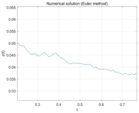
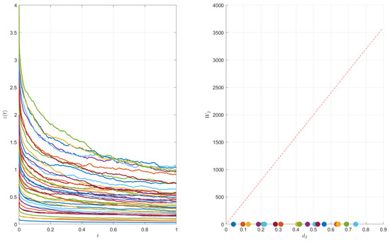
From Equation (29), $C=1.6\ast {10}^7$. It follows from Theorem 2 that the transportation inequality holds when $W<\sqrt{C}{d}_2$ holds. Taking $2^{-10}$ as the step, Euler’s method was used to obtain the approximate solution of the equation, as shown in Figure 1. As shown in the left side of Figure 2, we selected 20 groups of paths with different initial values. The right graph of Figure 2 shows $(W_2,d_2)$ and the theoretical upper bound $\sqrt{C}{d}_2$ associated with these 20 sets of paths. From the graph, we can see that $W_2$ is much smaller than $\sqrt{C}{d}_2$, which further supports our theoretical result (Theorem 2).

Figure 1. Euler method with step size $2^{-10}$. Partial path diagram of $z\left(t\right)$.

Figure 2. Path diagram (left), $W_2$ and theoretical upper bound (red line) (right).

References

- Yang, Z.; Zheng, X.; Wang, H. A variably distributed-order time-fractional diffusion equation: Analysis and approximation. Comput. Methods Appl. Mech. Eng. 2020, 367, 113118. [Google Scholar] [CrossRef]
- Bao, H.; Park, J.H.; Cao, J. Adaptive synchronization of fractional-order output-coupling neural networks via quantized output control. IEEE Trans. Neural Netw. Learn. Syst. 2021, 32, 3230–3239. [Google Scholar] [CrossRef] [PubMed]
- Diethelm, K. The Analysis of Fractional Differential Equations. An Application-Oriented Exposition Using Differential Operators of Caputo Type; Springer: Berlin/Heidelberg, Germany, 2024. [Google Scholar]
- Li, C.; Li, Z. The finite-time blow-up for semilinear fractional diffusion equations with time ψ-Caputo derivative. J. Nonlinear Sci. 2022, 32, 1–42. [Google Scholar] [CrossRef]
- Ahmadova, A.; Mahmudov, N. Existence and uniqueness results for a class of fractional stochastic neutral differential equations. Chaos Solitons Fractals 2020, 139, 110253. [Google Scholar] [CrossRef]
- Kilbas, A.; Srivastava, H.; Trujillo, J. Theory and Applications of Fractional Differential Equations; Elsevier: Amsterdam, The Netherlands, 2006; Volume 204. [Google Scholar]
- Samko, S.; Kilbas, A.; Marichev, O. Fractional Integrals and Derivatives: Theory and Applications; Gordon and Breach Publishers: London, UK, 1993. [Google Scholar]
- Xu, L.; Li, Z. Stochastic fractional evolution equations with fractional brownian motion and infinite delay. Appl. Math. Comput. 2018, 336, 36–46. [Google Scholar] [CrossRef]
- Yang, Z.; Wang, H. Strong convergence of a Euler-Maruyama scheme to a variable-order fractional stochastic differential equation driven by a multiplicative white noise. Chaos Solitons Fractals 2021, 142, 110392. [Google Scholar] [CrossRef]
- Dong, J.; Du, N.; Yang, Z. A distributed-order fractional stochastic differential equation driven by Lévy noise: Existence, uniqueness, and a fast EM scheme. Chaos Interdiscip. J. Nonlinear Sci. 2023, 33, 023109. [Google Scholar] [CrossRef]
- Lorenzo, C.; Hartley, T. Variable order and distributed order fractional operators. Nonlinear Dyn. 2002, 29, 57–98. [Google Scholar] [CrossRef]
- Patnaik, S.; Hollkamp, J.; Semperlotti, F. Applications of variable-order fractional operators: A review. Proc. R. Soc. A 2020, 476, 20190498. [Google Scholar] [CrossRef]
- Sun, H.; Chen, W.; Chen, Y. Variable-order fractional differential operators in anomalous diffusion modeling. Phys. A Stat. Mech. Its Appl. 2009, 388, 4586–4592. [Google Scholar] [CrossRef]
- Sun, H.; Chang, A.; Zhang, Y. A review on variable-order fractional differential equations: Mathematical foundations, physical models, numerical methods and applications. Fract. Calc. Appl. Anal. 2019, 22, 27–59. [Google Scholar] [CrossRef]
- Diethelm, K.; Ford, N. Numerical analysis for distributed-order differential equations. J. Comput. Appl. Math. 2009, 225, 96–104. [Google Scholar] [CrossRef]
- Mainardi, F.; Pagnini, G.; Gorenflo, R. Some aspects of fractional diffusion equations of single and distributed order. Appl. Math. Comput. 2007, 187, 295–305. [Google Scholar]
- Boufoussi, B.; Hajji, S. Neutral stochastic functional differential equations driven by a fractional Brownian motion in a Hilbert space. Stat. Probab. Lett. 2012, 82, 1549–1558. [Google Scholar] [CrossRef]
- Caraballo, T.; Garrido-Atienza, M.; Taniguchi, T. The existence and exponential behavior of solutions to stochastic delay evolution equations with a fractional Brownian motion. Nonlinear Anal. Theory Methods Appl. 2011, 74, 3671–3684. [Google Scholar] [CrossRef]
- Li, Z. Shift Harnack inequality and integration by parts formula for functional SDEs driven by fractional Brownian motion. Proc. Am. Math. Soc. 2016, 144, 2651–2659. [Google Scholar] [CrossRef]
- Li, Z.; Yan, L. Stochastic averaging for two-time-scale stochastic partial differential equations with fractional Brownian motion. Nonlinear Anal. Hybrid Syst. 2019, 31, 317–333. [Google Scholar] [CrossRef]
- Li, Z.; Xu, L.; Zhou, J. Viability for coupled SDEs driven by fractional Brownian motion. Appl. Math. Optim. 2021, 84, 55–98. [Google Scholar] [CrossRef]
- Shen, G.; Xiang, J.; Wu, J. Averaging principle for distribution dependent stochastic differential equations driven by fractional Brownian motion and standard Brownian motion. J. Differ. Equ. 2022, 321, 381–414. [Google Scholar] [CrossRef]
- Xu, J.; Lian, Q.; Wu, J. A strong averaging principle rate for two-time-scale coupled forward–backward stochastic differential equations driven by fractional Brownian motion. Appl. Math. Optim. 2023, 88, 32. [Google Scholar] [CrossRef]
- Xu, J.; Sun, Y.; Ren, J. A support theorem for stochastic differential equations driven by a fractional Brownian motion. J. Theor. Probab. 2022, 36, 728–761. [Google Scholar] [CrossRef]
- Djellout, H.; Guillin, A.; Wu, L. Transportation cost-information inequalities and applications to random dynamical systems and diffusions. Ann. Probablity 2004, 32, 2702–2732. [Google Scholar] [CrossRef]
- Wu, L.; Zhang, Z. Talagrand’s T2-transportation inequality w.r.t. a uniform metric for diffusions. Acta Math. Appl. Sin. 2004, 20, 357–364. [Google Scholar] [CrossRef]
- Wu, L.; Zhang, Z. Talagrand’s T2-transportation inequality and log-sobolev inequality for dissipative SPDEs and applications to reaction-diffusion equations. Chin. Ann. Math. Ser. B 2006, 27, 243–262. [Google Scholar] [CrossRef]
- Ma, Y. Transportation inequalities for stochastic differential equations with jumps. Stoch. Processes Their Appl. 2010, 120, 2–21. [Google Scholar] [CrossRef]
- Wu, L. Transportation inequalities for stochastic differential equations of pure jumps. Ann. l’IHP Probab. Stat. 2010, 46, 465–479. [Google Scholar] [CrossRef]
- Pal, S. Concentration for multidimensional diffusions and their boundary local times. Probab. Theory Relat. Fields 2012, 154, 225–254. [Google Scholar] [CrossRef]
- Saussereau, B. Transportation inequalities for stochastic differential equations driven by a fractional Brownian motion. Bernoulli 2012, 18, 1–23. [Google Scholar] [CrossRef]
- Li, Z.; Luo, J. Transportation inequalities for stochastic delay evolution equations driven by fractional Brownian motion. Front. Math. China 2015, 10, 303–321. [Google Scholar] [CrossRef]
- Boufoussi, B.; Hajji, S. Transportation inequalities for neutral stochastic differential equations driven by fractional Brownian motion with Hurst parameter less than 1/2. Mediterr. J. Math. 2017, 14, 192. [Google Scholar] [CrossRef]
- Mishura, Y.; Mishura, I. Stochastic Calculus for Fractional Brownian Motion and Related Processes; Springer Science & Business Media: Berlin/Heidelberg, Germany, 2008; Volume 1929. [Google Scholar]
- Hu, Y.; Øksendal, B. Fractional white noise calculus and applications to finance. Infin. Dimens. Anal. Quantum Probab. Relat. Top. 2003, 6, 1–32. [Google Scholar] [CrossRef]
- Biagini, F.; Hu, Y.; Øksendal, B.; Zhang, T. Stochastic Calculus for Fractional Brownian Motion and Applications; Springer Science & Business Media: Berlin/Heidelberg, Germany, 2008. [Google Scholar]
- Alos, E.; Mazet, O.; Nualart, D. Stochastic calculus with respect to Gaussian processes. Ann. Probab. 2001, 29, 766–801. [Google Scholar] [CrossRef]
- Rascanu, A. Differential equations driven by fractional Brownian motion. Collect. Math. 2002, 53, 55–81. [Google Scholar]
- Holden, H.; Øksendal, B.; Ubøe, J.; Zhang, T.; Holden, H. Stochastic Partial Differential Equations; Springer: Berlin/Heidelberg, Germany, 1996. [Google Scholar]
- Karatzas, I.; Shreve, S. Brownian Motion and Stochastic Calculus; Springer: Berlin/Heidelberg, Germany, 2014; Volume 113. [Google Scholar]
- Xu, Y.; Pei, B.; Wu, J. Stochastic averaging principle for differential equations with non-Lipschitz coefficients driven by fractional Brownian motion. Stochastics Dyn. 2017, 17, 1750013. [Google Scholar] [CrossRef]
- Prato, G.; Zabczyk, J. Stochastic Equations in Infinite Dimensions; Cambridge University Press: Cambridge, UK, 2008. [Google Scholar]
Disclaimer/Publisher’s Note: The statements, opinions and data contained in all publications are solely those of the individual author(s) and contributor(s) and not of MDPI and/or the editor(s). MDPI and/or the editor(s) disclaim responsibility for any injury to people or property resulting from any ideas, methods, instructions or products referred to in the content. |
© 2025 by the authors. Licensee MDPI, Basel, Switzerland. This article is an open access article distributed under the terms and conditions of the Creative Commons Attribution (CC BY) license (https://creativecommons.org/licenses/by/4.0/).