Abstract
This study presents a novel fractional-order mathematical model to investigate zoonotic disease transmission between humans and baboons, incorporating the Generalized Euler Method and highlighting key control strategies such as sterilization, restricted food access, and reduced human–baboon interaction. The model’s structure exhibits an inherent symmetry in the transmission dynamics between baboon and human populations, reflecting balanced interaction patterns. This symmetry is further analyzed through the stability of infection-free and endemic equilibrium points, guided by the basic reproduction number . Theoretical analyses confirmed the existence, uniqueness, and boundedness of solutions, while sensitivity analysis identified critical parameters influencing disease spread. Numerical simulations validated the effectiveness of intervention strategies, demonstrating the impact of symmetrical measures on minimizing zoonotic disease risks and promoting balanced population health outcomes. This work contributes to epidemiological modeling by illustrating how symmetry in control interventions can optimize zoonotic disease management.
1. Introduction
Zoonotic diseases, or infections that are transmitted between animals and humans, represent a significant public health challenge worldwide [1]. As human activities increasingly encroach on wildlife habitats, the risk of zoonotic disease transmission has escalated [2]. Among the various species that can act as reservoirs for zoonotic diseases, baboons (genus Papio) are notable for their frequent interactions with human populations, particularly in regions like Al-Baha, Saudi Arabia [3]. These interactions, often resulting from competition for food and habitat, create opportunities for the transmission of diseases that can spread between humans and baboons [4].
In the Al-Baha region, the presence of baboons has been linked to potential zoonotic outbreaks, largely due to their proximity to human settlements and the overlap in resource use [5]. Diseases such as tuberculosis and other viral infections, which can be transmitted through direct contact or contaminated resources, pose a serious risk to both baboon and human populations [6]. Moreover, the behavior of feeding baboons, particularly by local residents and tourists, exacerbates this interaction, increasing the chances of zoonotic disease transmission [7].
Mathematical modeling plays a crucial role in analyzing disease transmission dynamics in both human and animal populations [8]. These models enable the examination of intricate relationships by simulating various parameters, such as population density, disease spread rates, and preventive interventions, to better understand disease behavior [9]. This research adopts a modeling framework to capture the transmission dynamics of zoonotic diseases between baboons and humans in the Al-Baha region. By combining mathematical approaches with real-world data, we aim to enhance knowledge of zoonotic infections and aid public health initiatives in mitigating outbreak risks. The outcomes of this study also hold potential significance for managing wildlife populations and controlling infectious diseases in regions characterized by frequent human-animal interactions [10].
In recent years, fractional calculus has emerged as a powerful tool for describing systems that exhibit memory and hereditary properties [11]. Its growing popularity is evident in fields such as engineering [12], plant pathology [13], biology [14], medicine [15], behavioral sciences [16], viscoelastic materials [17], electromagnetic waves [18], quantum mechanics [19], Langevin equations [20], physics [21,22,23,24], diabetes modeling [25,26,27,28,29,30,31], cybersecurity [32], smoking dynamics [33], epidemiology [34,35], influenza [36], infectious disease outbreaks [37], epidemic modeling [38], cancer research [39], COVID-19 [40], monkeypox [41], zoonotic viruses [42], and alcohol-related studies [43]. Epidemiological models, in particular, have found extensive applications in various disciplines, such as healthcare, chemistry, physics, and economic modeling [44,45,46,47,48,49,50,51,52,53]. Sadek et al. (2024) expanded fractional calculus by proposing innovative -fractional operators and demonstrating their effectiveness in optimization problems using the Galerkin-Bell technique [49]. In a related contribution, Sadek (2023) introduced a cotangent-based fractional derivative, offering an alternative framework for solving complex differential equations [50]. Building on this concept, Sadek and Lazar (2023) applied the Hilfer cotangent fractional operator to a specialized set of problems, bridging classical and fractional calculus perspectives [51]. In epidemiology, Sadek et al. (2023) proposed a fractional-order COVID-19 model for Morocco that incorporated vaccination and isolation measures, enhancing accuracy by accounting for memory effects [52]. Additionally, Sadek et al. (2022) utilized fractional calculus to describe the low-temperature synthesis of TiO2 nanopowder via the sol-gel technique, improving nanomaterial production models [53]. These advancements underscore fractional calculus’ versatility across multiple scientific domains.
Compared to traditional integer-order models, fractional calculus provides distinct advantages when describing dynamic systems. Despite this, solving fractional differential equations (FDEs) analytically can be highly challenging, necessitating numerical methods. Numerous techniques have been developed to approximate FDE solutions. For instance, the generalized Euler scheme [54,55] efficiently handles Caputo-type FDEs and is relatively simple to implement. However, it may not be suitable for solving higher-order equations. Other numerical approaches, including the Adomian decomposition method [56], the homotopy perturbation method [57,58], the homotopy analysis method [59,60], the Taylor matrix technique [61,62], and the Haar wavelet approach [63], have been successfully employed to study fractional systems.
This research focuses on understanding the transmission dynamics of zoonotic diseases in a baboon-human population system, while integrating control measures such as sterilization, food access restriction, and minimizing human-baboon interactions [64]. The mathematical analysis ensures the model’s reliability by demonstrating the existence, uniqueness, positivity, and boundedness of its solutions [65]. Furthermore, the basic reproductive number () is calculated to evaluate the likelihood of disease outbreak or eradication [66]. Sensitivity analysis identifies critical parameters affecting disease spread, offering guidance for designing effective control strategies [67].
This study introduces a fractional-order epidemiological model for zoonotic disease transmission between baboons and humans, with a focus on key interventions, including sterilization, limiting food access, and reducing contact. A rigorous mathematical examination confirms the model’s well-posedness by establishing solution properties such as existence, uniqueness, and positivity. The basic reproductive number () is derived to assess the conditions under which the disease persists or is eliminated. A sensitivity analysis pinpoints influential factors affecting disease dynamics. Additionally, the numerical solutions of the fractional-order system are approximated using the Generalized Euler Method, which is known for its computational efficiency and accuracy in solving FDEs. The simulations provide valuable insights into the potential impact of various control strategies on reducing zoonotic disease risk.
The remainder of this paper is structured as follows: Section 2 describes the model formulation, including fractional-order differential equations. Section 3 provides a theoretical analysis of the model and its well-posedness. Section 4 discusses the equilibrium stability and computation of . Section 5 outlines the numerical approach, specifically the Generalized Euler Method. Finally, Section 6 interprets the results, and Section 7 concludes with recommendations for future work.
2. Baboon and Human Population Model Description
The following model aims to simulate the dynamics of baboon and human populations in the context of zoonotic disease transmission. The model incorporates control strategies such as sterilization, restricted food access, and reduced human–baboon interactions. The baboon population dynamics are modeled using the following equations, where we account for natural growth, disease transmission, and control actions. The combined system of equations modeling the dynamics of baboon and human populations with zoonotic disease transmission is as follows:
The variables and parameters used in the baboon-human disease framework are defined as follows: , , and represent the susceptible, infected, and recovered populations of baboons, respectively. Likewise, , , and denote the corresponding human populations. The key parameters include r, the natural growth rate of the baboon population; K, the carrying capacity based on the availability of resources; , the disease transmission rate within the baboon population; , the transmission rate from baboons to humans; , the recovery rate of infected baboons; and , the recovery rate of infected humans.
Additionally, , , and represent control interventions targeting the baboon population, specifically sterilization measures, food restriction, and reduction in human contact, respectively. These definitions form the foundation for understanding the dynamics of disease transmission between baboons and humans within the model.
The fractional-order formulation of the model, for , is given by:
The parameters in the fractional-order model were determined through empirical data, assumptions, and numerical calibration. Epidemiological data from the Al-Baha region informed estimates for key parameters such as the transmission rate from baboons to humans () and the human recovery rate (), while control parameters () were based on plausible intervention strategies and validated through sensitivity analysis. Numerical simulations ensured the model outputs aligned with observed disease dynamics.
3. Foundational Concepts
This section presents key definitions and some fundamental properties of fractional calculus. Let denote the set of non-negative real numbers. For any fractional order , the fractional integral of a function is defined by
where is the Euler Gamma function.
Definition 1
([68]). The Caputo fractional derivative of order for , where and , is given by:
Consider the following fractional-order initial value problem:
where denotes the Caputo fractional derivative, and is a vector function. Let be a complete metric space under an appropriate norm , and define:
Lemma 1
([69]). Let be a function satisfying the following conditions:
- (1)
- is Lebesgue measurable in t on ,
- (2)
- is continuous in Z on ,
- (3)
- There exists a function such that:for almost every and all ,
- (4)
- There is a function such that:for almost every and any .
Lemma 2
([70]). Assume that satisfies the following criteria:
- (1)
- is Lebesgue measurable with respect to t on ,
- (2)
- is continuous in Z on ,
- (3)
- The partial derivative is continuous on ,
- (4)
- There exist constants and such that:for almost every and all .
Lemma 3
([71,72]). Let be a function for which exists and satisfies the following inequality:
where , , and . Then:
where denotes the Mittag-Leffler function.
4. Existence, Uniqueness, and Positivity of Solution
Let us consider the domain of interest as follows:
In this region, the system possesses a unique, non-negative, and bounded solution.
Theorem 1.
Given any initial state , the system’s solution remains in Ψ for all and is unique.
Proof.
Define the vector-valued function , where each component is expressed as:
Now, for any , we have:
where
Since adheres to the Lipschitz condition, it follows that the solution to the given system exists and is unique. □
Theorem 2.
If the initial values satisfy , , , , , and , then the solution of system (1) remains non-negative for all .
Proof.
To demonstrate this, we evaluate the right-hand side of the system at the respective boundaries:
Since all the evaluated terms are either zero or non-negative at , , , , , and , none of the variables can drop below zero. Hence, the solution remains non-negative for all . By applying standard results on the positivity of differential equations, it follows that the non-negativity of the solution is preserved throughout the evolution of the system. □
Theorem 3.
The solutions of system (1) are uniformly bounded within the region
where the parameter λ is defined as .
Proof.
Define a function representing the total population size at any time t:
By adding all the equations in the system, we obtain:
Since , we can establish the following upper bound for :
Thus, we have:
Following the approach outlined in [73], we obtain:
where represents the Mittag-Leffler function. Considering the asymptotic behavior of this function as derived in [74], we further conclude:
Hence, if the initial conditions place the solutions within , they remain uniformly bounded inside the region over time. □
Remark 1.
The set Ω is positively invariant under the dynamics of the system, meaning that any solution that starts in Ω will remain within this bounded region.
5. Equilibrium Points and Stability
At equilibrium, we solve for and , with , leading to the infection-free equilibrium:
where
According to the framework presented in [75], the basic reproduction number is expressed as
Lemma 4.
The equilibrium point is LAS within the domain Ω when , but it becomes unstable if .
Proof.
At the disease-free equilibrium , the Jacobian matrix associated with system (1) takes the form:
The characteristic equation for this matrix can be derived as follows:
Thus, the eigenvalues are
For stability, all eigenvalues must have negative real parts. and are always negative. The eigenvalues and depend on the basic reproduction number :
If , then and , and is LAS. If , then or , and is unstable. □
Theorem 4.
The equilibrium point is GAS.
Proof.
Let us define a LF that is positive definite as follows:
From Lemma 4, one obtains
Hence, it follows that holds for all . Additionally, the condition leads to . Thus, the equilibrium point forms the unique invariant set such that
Applying the fractional LaSalle Invariance Principle [76,77] and utilizing the result from Lemma 3, the equilibrium is GAS within the domain . □
For , represents the endemic equilibrium, corresponding to the steady-state solution of the given model. Using the steady-state conditions:
and substituting from the second and third equations, we express and :
By inserting this result into the fourth equation, we find:
Now, substituting this into the first equation, we solve for :
Thus, the endemic equilibrium can be expressed as:
Lemma 5.
If , is LAS in Ω.
Proof.
For the first-order integer model, the Jacobian matrix at is given by
Evaluating the Jacobian matrix at gives the characteristic equation
where I is the identity matrix. The characteristic polynomial is
where the coefficients are defined in terms of the parameters of the model.
If the Routh–Hurwitz criterion is satisfied, the endemic equilibrium is locally stable:
Thus, is LAS when , as all conditions of the Routh–Hurwitz criterion are satisfied. □
Theorem 5.
The positive endemic equilibrium point of the model is GAS.
Proof.
Consider this positive definite LF:
From Lemma 4, one obtains
Thus, for all . Furthermore, implies that , , , , , and . Therefore, the singleton is the only invariant set such that .
Applying the fractional LaSalle Invariance Principle and using Lemma 3, is GAS on . □
6. Utilization of the Extended Euler Approach
Based on a framework inspired by fractional numerical schemes, we implement a generalized Euler technique to approximate the solutions of the proposed system. Let us examine the fractional-order differential equation:
The interval is partitioned into k segments of equal width , with discretization points for . Utilizing the fractional Taylor series expansion and assuming that x, , and are continuous on , we can write:
By substituting and ignoring the second-order term for sufficiently small h, we derive:
For small step size h, the term involving becomes negligible, yielding:
By repeating this process, we generate a sequence of approximate solutions . For , the generalized Euler formula becomes:
for . Notably, when , this method simplifies to the classical Euler scheme.
Applying this extended numerical approach (3) to the given system (1) leads to the following iterative expressions:
where the parameter serves as the step size. The initial values are , , , , , and .
This extended numerical scheme offers an effective tool for approximating fractional dynamics while maintaining computational efficiency.
6.1. Numerical Experiments
This part presents the implementation of the Modified Euler Approach to numerically estimate the solutions of the fractional-order zoonotic disease framework. This numerical scheme is specifically advantageous for fractional differential systems due to its ability to maintain computational accuracy while capturing the memory-dependent effects intrinsic to fractional calculus. The simulations investigate how various control interventions—such as sterilizing baboons, restricting food availability, and minimizing human–baboon encounters—affect disease transmission patterns.
For the simulations, real-world data on zoonotic disease transmission between humans and baboons in Al-Baha were incorporated, as reported by the Ministry of Environment, Agriculture, and Water in Saudi Arabia’s Al-Baha region. The parameter values and their respective sources are summarized in Table 1, with initial population values set as follows: , , , , , and .

Table 1.
Parameter values and initial conditions used in the zoonotic disease model [78].
To analyze the dynamics of disease transmission, we conducted simulations under various control scenarios. The model parameters were selected based on empirical estimates from epidemiological studies in the Al-Baha region, where frequent human–baboon interactions contribute to zoonotic disease spread. The key findings from our simulations are summarized below:
- Baseline Dynamics: Without any control interventions, the infected baboon () and infected human () populations exhibited sustained growth, leading to persistent zoonotic disease transmission. The basic reproduction number remained above 1, indicating an endemic situation.
- Effect of Sterilization (): Increasing the sterilization rate of baboons significantly reduced the susceptible baboon population (), thereby lowering the overall infection rate. However, sterilization alone was not sufficient to eliminate the disease entirely, as transmission still occurred through infected individuals.
- Effect of Food Access Restriction (): Limiting food availability for baboons decreased human–baboon interactions, leading to a decline in transmission. The simulations showed that moderate values of contributed to a substantial reduction in both and , making this an effective intervention strategy.
- Effect of Reducing Human–Baboon Interaction (): Implementing measures such as public awareness campaigns and habitat modifications reduces direct contact between baboons and humans. The simulations revealed that increasing led to a significant decline in , confirming that minimizing interaction is one of the most effective strategies for controlling zoonotic disease spread.
- Combined Control Strategies: The most effective disease mitigation was achieved when sterilization, food restriction, and interaction reduction were applied simultaneously. In such cases, the model predicted that dropped below 1, leading to disease eradication over time.
The numerical simulations in this study explored the dynamics of zoonotic disease transmission between baboons and humans under various control scenarios. The simulations focused on how changes in control measures, represented by the parameters , , and , impacted susceptible, infected, and recovered populations for both baboons and humans. These parameters correspond to sterilization, food access restriction, and interaction reduction controls, respectively. Below is an interpretation of each figure in the manuscript, followed by explanations of the trends and outcomes observed in each simulation.
Figure 1 examine how different levels of the control parameters , , and affect the infected baboon population. In Figure 1a shows that increasing gradually reduced the infected baboon population , indicating that sterilization effectively limits disease spread. Figure 1b displays a similar trend for varying , suggesting that restricting food access significantly decreases infection rates by reducing contact around food sources. Figure 1c illustrates that increased human interaction control () lowers infection levels in baboons, demonstrating the importance of minimizing contact between humans and baboons to prevent disease spillover.
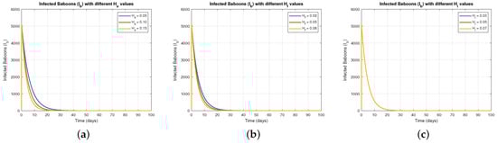
Figure 1.
The effect of varying on .
Figure 2 explores the impact of different control intensities , , and on the infected human population (). Figure 2a demonstrates that increasing exerts minimal direct influence on , since sterilization primarily impacts baboons. Figure 2b indicates that food restriction () effectively reduces , as limiting food availability curtails baboon-human encounters. Figure 2c highlights that increased values substantially lower , underlining the critical role of minimizing human-baboon interactions in controlling zoonotic transmission.
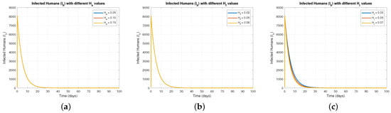
Figure 2.
The effect of varying on .
Figure 3 focuses on how control measures , , and affect the recovered baboon population (). Figure 3a shows that increasing results in a steady rise in , as more baboons recover due to reduced transmission. Figure 3b,c depict similar recovery trends with higher values of and , confirming that effective control measures reduce infection and enhance recovery rates.
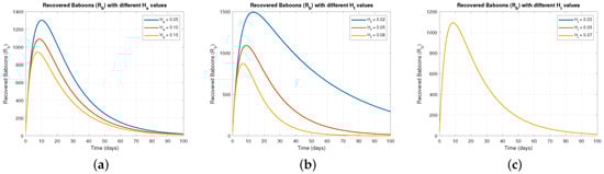
Figure 3.
The effect of varying on .
Figure 4 focuses on how control measures , , and affect the recovered baboon population (). Figure 4a shows that increasing results in a steady rise in , as more baboons recover due to reduced transmission. Figure 4b,c depict similar recovery trends with higher values of and , confirming that effective control measures reduce infection and enhance recovery rates.
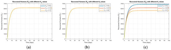
Figure 4.
The effect of varying on .
Figure 5 illustrates the population dynamics of baboons in different compartments—, , , , , —under varying fractional-order . The subfigures (a–f) within Figure 5 focus on how different initial control parameter values influence the overall population trajectories:
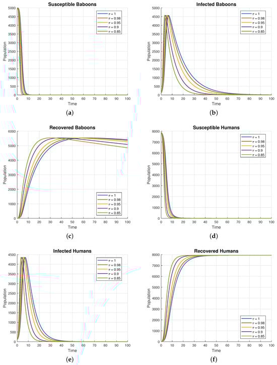
Figure 5.
Time series plot of respectively, with various fractional-order .
6.2. Error Estimation
In this section, we estimate the convergence rate of our six-component numerical scheme. Convergence rate is determined by
where , , and are the approximate solutions for step sizes h, , and , respectively.
Table 2, Table 3 and Table 4 indicate the rate of convergence, typically approaching first-order and second-order accuracy. However, chaotic systems, like the one studied, are highly sensitive to initial conditions, so these results may exhibit variations due to the nature of the system.
Table 2.
The rate of convergence for different values of h for and .
Table 3.
The rate of convergence for different values of h for and .
Table 4.
The rate of convergence for different values of h for and .
7. Discussion
This study presents a fractional-order mathematical model to analyze zoonotic disease transmission between baboons and humans, incorporating control measures such as sterilization, food access restriction, and reduced human–baboon interactions. The mathematical model developed in this study highlights the complex interactions between baboon and human populations, concerning zoonotic disease transmission. The inclusion of fractional-order derivatives allows the model to account for memory and hereditary properties inherent in biological systems, providing a more accurate representation of disease dynamics compared to traditional models. The stability analysis of the infection-free and endemic equilibrium points confirmed that the basic reproduction number is a critical determinant of disease persistence or eradication. A basic reproduction number less than one indicates that the disease will eventually be eradicated, while a value greater than one suggests the disease may persist. The sensitivity analysis identified critical parameters, such as the transmission rates between baboons and humans and the recovery rates of both populations. Interventions that reduced human–baboon contact, such as sterilization and limiting access to food resources, proved to be effective in lowering transmission rates. The findings underscore the importance of combining these control measures with public health strategies aimed at improving human recovery rates through medical interventions. The numerical simulations conducted in this study supported the theoretical results, demonstrating that optimal control strategies can significantly reduce zoonotic disease risks. Sterilization of baboons, along with restricted food access and reduced interactions with humans, emerged as an effective approach for controlling zoonotic disease transmission.
The numerical simulations confirmed the effectiveness of various intervention strategies in controlling zoonotic disease transmission. Notably, reducing human–baboon interactions () played a crucial role in mitigating infections, while food restriction () emerged as a practical and impactful control measure. The Generalized Euler Method provided a robust numerical framework for approximating the fractional-order system, ensuring accurate predictions of disease dynamics. These findings highlight the importance of integrating mathematical modeling with public health policies to design optimal zoonotic disease control strategies.
The feasibility of implementing control measures for human–baboon interactions involves assessing sterilization, food restriction, and interaction reduction, each with unique challenges and potential solutions. Sterilization, while moderately feasible, is resource-intensive, ethically complex, and slow in impact, though alternatives such as immunocontraceptives and small-scale trials may enhance effectiveness. Food restriction is more practical, requiring secured waste disposal and public education, though enforcement must be sustained to prevent baboons from seeking alternative food sources. Reducing human–baboon interactions is similarly feasible but demands long-term public behavioral change, supported by wildlife corridors, deterrents, and fines for feeding. Empirical studies, including macaque sterilization in urban areas, bear-proofing programs in North America, and eco-tourism regulations in Kruger National Park, provide valuable validation of these interventions. A multi-faceted approach combining these strategies, alongside education, community engagement, and continuous monitoring, offers the most effective solution for mitigating human–baboon conflicts.
The stability analysis confirmed that the basic reproduction number () is a critical threshold for disease persistence, with leading to eradication and indicating endemic conditions. The sensitivity analysis highlighted that transmission and recovery rates significantly influence disease spread. Numerical simulations using the Generalized Euler Method demonstrated that food access restriction () and interaction reduction () were particularly effective in controlling the disease, while sterilization () alone was insufficient. The Generalized Euler Method provided computational efficiency and accuracy in approximating the fractional-order system, confirming its suitability for complex epidemiological modeling. The results underscore the importance of integrating mathematical modeling with public health strategies, such as limiting human–wildlife interactions, promoting awareness campaigns, and implementing wildlife management policies. Future work should incorporate spatial dynamics, refine parameter estimates using empirical data, and explore alternative numerical methods to enhance predictive accuracy. Overall, this research contributes to a deeper understanding of zoonotic disease control and informs evidence-based intervention strategies.
8. Conclusions
This study developed a fractional-order mathematical model to investigate zoonotic disease transmission between baboons and humans, incorporating key control strategies such as sterilization, food access restriction, and reduced human–baboon interactions. Theoretical analysis established the model’s well-posedness, including the existence, uniqueness, non-negativity, and boundedness of solutions. The basic reproduction number () was derived to assess disease persistence, confirming that leads to eradication, while results in endemic conditions. A sensitivity analysis identified critical parameters influencing transmission, emphasizing the effectiveness of intervention measures. Numerical simulations using the Generalized Euler Method demonstrated that reducing human–baboon interactions () and restricting food access () significantly lowered infection rates, while sterilization () contributed to long-term control but was less effective as a standalone measure. The study highlights the importance of integrating mathematical modeling with public health policies, to develop optimal zoonotic disease management strategies. Future research should extend the model by incorporating spatial dynamics, refining parameter estimates using real-world data, and exploring alternative numerical schemes for improved computational efficiency. The findings provide valuable insights for policymakers and wildlife management authorities to implement targeted interventions and mitigate zoonotic disease risks.
Author Contributions
Conceptualization, S.S.; Methodology, S.S.; Software, S.S. and E.S.; Validation, S.S.; Formal analysis, S.S.; Investigation, S.S.; Resources, S.S. and E.S.; Data curation, S.S. and E.S.; Writing—original draft, S.S. and E.S.; Writing—review & editing, S.S. and E.S. All authors have read and agreed to the published version of the manuscript.
Funding
This research was supported and funded by the Deanship of Scientific Research at Imam Mohammad Ibn Saud Islamic University (IMSIU) (grant number IMSIU-DDRSP2501).
Data Availability Statement
Data is contained within the article.
Acknowledgments
This research was supported and funded by the Deanship of Scientific Research at Imam Mohammad Ibn Saud Islamic University (IMSIU) (grant number IMSIU-DDRSP2501).
Conflicts of Interest
The authors declare no conflicts of interest.
References
- Jones, K.E.; Patel, N.G.; Levy, M.A.; Storeygard, A.; Balk, D.; Gittleman, J.L.; Daszak, P. Global trends in emerging infectious diseases. Nature 2008, 451, 990–993. [Google Scholar] [CrossRef] [PubMed]
- Woolhouse, M.E.; Gowtage-Sequeria, S. Host range and emerging and reemerging pathogens. Emerg. Infect. Dis. 2005, 11, 1842–1847. [Google Scholar] [CrossRef]
- Al-Aklabi, A.; Al-Khulaidi, A.W.; Hussain, A.; Al-Sagheer, N. Main vegetation types and plant species diversity along an altitudinal gradient of Al Baha region, Saudi Arabia. Saudi J. Biol. Sci. 2016, 23, 687–697. [Google Scholar] [CrossRef] [PubMed]
- Daszak, P.; Cunningham, A.A.; Hyatt, A.D. Emerging infectious diseases of wildlife–threats to biodiversity and human health. Science 2000, 287, 443–449. [Google Scholar] [CrossRef]
- Wolfe, N.D.; Dunavan, C.P.; Diamond, J. Origins of major human infectious diseases. Nature 2007, 447, 279–283. [Google Scholar] [CrossRef]
- Kock, R.A.; Wamwayi, H.; Rossiter, P.; Libeau, G.; Wambwa, E. Re-infection of wildlife populations with rinderpest virus on the periphery of the Somali ecosystem in East Africa. Prev. Vet. Med. 2006, 75, 63–80. [Google Scholar] [CrossRef] [PubMed]
- Drewe, J.A.; O’Riain, M.J.; Beamish, E.; Currie, H.; Parsons, S. Survey of infections transmissible between baboons and humans, Cape Town, South Africa. Emerg. Infect. Dis. 2012, 18, 298–301. [Google Scholar] [CrossRef]
- Van den Driessche, P.; Watmough, J. Reproduction numbers and subthreshold endemic equilibria for compartmental models of disease transmission. Math. Biosci. 2002, 180, 29–48. [Google Scholar] [CrossRef]
- Huo, J.; Zhao, H.; Zhu, L. The effect of vaccines on backward bifurcation in a order HIV model. Nonlinear Anal. Real World Appl. 2015, 26, 289–305. [Google Scholar] [CrossRef]
- Jones, B.A.; Grace, D.; Kock, R.; Alonso, S.; Rushton, J.; Said, M.Y.; McKeever, D.; Mutua, F.; Young, J.; McDermott, J.; et al. Zoonosis emergence linked to agricultural intensification and environmental change. Proc. Natl. Acad. Sci. USA 2013, 110, 8399–8404. [Google Scholar] [CrossRef]
- Atangana, A.; Baleanu, D. New fractional derivatives with non-local and non-singular kernel: Theory and application to heat transfer model. Therm. Sci. 2016, 20, 763–769. [Google Scholar]
- Arena, P.; Caponetto, R.; Fortuna, L.; Porto, D. Nonlinear Noninteger Order Circuits and Systems; World Scientific: Singapore, 2000. [Google Scholar]
- Nisar, K.S.; Farman, M.; Abdel-Aty, M.; Ravichandran, C. A review of fractional-order models for plant epidemiology. Progr. Fract. Differ. Appl. 2024, 10, 489–521. [Google Scholar]
- Ahmed, E.; Elgazzar, A.S. On fractional order differential equations model for nonlocal epidemics. Phys. A Stat. Mech. Its Appl. 2007, 379, 607–614. [Google Scholar]
- Li, W.; Wang, Y.; Cao, J.; Abdel-Aty, M. Dynamics and backward bifurcations of SEI tuberculosis models in homogeneous and heterogeneous populations. J. Math. Anal. Appl. 2025, 543, 128924. [Google Scholar]
- Nisar, K.S.; Farman, M.; Abdel-Aty, M.; Ravichandran, C. A review of fractional order epidemic models for life sciences problems: Past, present and future. Alex. Eng. J. 2024, 95, 283–305. [Google Scholar]
- Bagley, R.L.; Calico, R.A. Fractional order state equations for the control of viscoelastically damped structures. J. Guid. Control Dyn. 1991, 14, 304–311. [Google Scholar]
- Heaviside, O. Electromagnetic Theory; Chelsea: New York, NY, USA, 1971. [Google Scholar]
- Kusnezov, D.; Bulgac, A.; Dang, G.D. Quantum levy processes and fractional kinetics. Phys. Rev. Lett. 1999, 82, 1136. [Google Scholar]
- Hammad, H.A.; Qasymeh, M.; Abdel-Aty, M. Existence and stability results for a Langevin system with Caputo–Hadamard fractional operators. Int. J. Geom. Methods Mod. Phys. 2024, 21, 2450218. [Google Scholar]
- Hilfer, R. Applications of Fractional Calculus in Physics; World Scientific: Singapore, 2000. [Google Scholar]
- Alsulami, A.; Alharb, R.A.; Albogami, T.M.; Eljaneid, N.H.; Adam, H.D.; Saber, S.F. Controlled chaos of a fractal–fractional Newton-Leipnik system. Therm. Sci. 2024, 28, 5153–5160. [Google Scholar]
- Yan, T.; Alhazmi, M.; Youssif, M.Y.; Elhag, A.E.; Aljohani, A.F.; Saber, S. Analysis of a Lorenz Model Using Adomian Decomposition and Fractal-Fractional Operators. Therm. Sci. 2024, 28, 5001–5009. [Google Scholar]
- Alhazmi, M.; Dawalbait, F.M.; Aljohani, A.; Taha, K.O.; Adam, H.D.; Saber, S. Numerical approximation method and Chaos for a chaotic system in sense of Caputo-Fabrizio operator. Therm. Sci. 2024, 28, 5161–5168. [Google Scholar]
- Sayed Saber, Safa Mirgani, Analyzing fractional glucose-insulin dynamics using Laplace residual power series methods via the Caputo operator: Stability and chaotic behavior. Beni-Suef Univ. J. Basic Appl. Sci. 2025, 14, 28. [CrossRef]
- Ahmed, K.I.; Adam, H.D.; Youssif, M.Y.; Saber, S. Different strategies for diabetes by mathematical modeling: Applications of fractal-fractional derivatives in the sense of Atangana-Baleanu. Results Phys. 2023, 52, 106892. [Google Scholar]
- Ahmed, K.I.; Adam, H.D.; Youssif, M.Y.; Saber, S. Different strategies for diabetes by mathematical modeling: Modified Minimal Model. Alex. Eng. J. 2023, 80, 74–87. [Google Scholar]
- Ahmed, K.I.A.; Mirgani, S.M.; Seadawy, A.; Saber, S. A comprehensive investigation of fractional glucose-insulin dynamics: Existence, stability, and numerical comparisons using residual power series and generalized Runge-Kutta methods. J. Taibah Univ. Sci. 2025, 19, 2460280. [Google Scholar]
- Saber, S.; Mirgani, S.M. Numerical Analysis and Stability of a Fractional Glucose-Insulin Regulatory System Using the Laplace Residual Power Series Method Incorporating the Atangana-Baleanu Derivative. Int. J. Model. Simul. Sci. Comput. 2025. [Google Scholar] [CrossRef]
- Alhazmi, M.; Saber, S. Glucose-insulin regulatory system: Chaos control and stability analysis via Atangana–Baleanu fractal-fractional derivatives. Alex. Eng. J. 2025, 122, 77–90. [Google Scholar]
- Saber, S.; Solouma, E.; Alharb, R.A.; Alalyani, A. Chaos in Fractional-Order Glucose–Insulin Models with Variable Derivatives: Insights from the Laplace–Adomian Decomposition Method and Generalized Euler Techniques. Fractal Fract. 2025, 9, 149. [Google Scholar] [CrossRef]
- Althubyani, M.; Saber, S. Hyers–Ulam Stability of Fractal–Fractional Computer Virus Models with the Atangana–Baleanu Operator. Fractal Fract. 2025, 9, 158. [Google Scholar] [CrossRef]
- Khan, H.; Alzabut, J.; Shah, A.; Etemad, S.; Rezapour, S.; Park, C. A study on the fractal-fractional tobacco smoking model. AIMS Math. 2022, 7, 13887–13909. [Google Scholar] [CrossRef]
- Khan, H.; Alzabut, J.; Tunç, O.; Kaabar, M.K. A fractal–fractional COVID-19 model with a negative impact of quarantine on the diabetic patients. Results Control Optim. 2023, 10, 100199. [Google Scholar]
- Almutairi, N.; Saber, S.; Ahmad, H. The fractal-fractional Atangana-Baleanu operator for pneumonia disease: Stability, statistical and numerical analyses. AIMS Math. 2023, 8, 29382–29410. [Google Scholar]
- Evirgen, F.; Uçar, E.; Uçar, S.; Özdemir, N. Modelling Influenza A disease dynamics under Caputo-Fabrizio fractional derivative with distinct contact rates. Math. Model. Numer. Simul. Appl. 2023, 3, 58–73. [Google Scholar]
- Ozdemir, N.; Uçar, E.; Avcı, D. Dynamic analysis of a fractional svir system modeling an infectious disease. Facta Univ. Ser. Math. Inform. 2022, 37, 605–619. [Google Scholar]
- Olumide, O.O.; Othman, W.A.M.; Özdemir, N. Efficient Solution of Fractional-Order SIR Epidemic Model of Childhood Diseases With Optimal Homotopy Asymptotic Method. IEEE Access 2022, 10, 9395–9405. [Google Scholar]
- Özdemir, N.; Uçar, E. Investigating of an immune system-cancer mathematical model with Mittag-Leffler kernel. AIMS Math. 2020, 5, 1519–1531. [Google Scholar] [CrossRef]
- Li, X.P.; Ullah, S.; Zahir, H.; Alshehri, A.; Riaz, M.B.; Al Alwan, B. Modeling the dynamics of coronavirus with super-spreader class: A fractal-fractional approach. Results Phys. 2022, 34, 105179. [Google Scholar]
- Alzubaidi, A.M.; Othman, H.A.; Ullah, S.; Ahmad, N.; Alam, M.M. Analysis of Monkeypox viral infection with human to animal transmission via a fractional and Fractal-fractional operators with power law kernel. Math. Biosci. Eng. 2023, 20, 6666–6690. [Google Scholar]
- Li, S.; Ullah, S.; Khan, I.U.; AlQahtani, S.A.; Riaz, M.B. A robust computational study for assessing the dynamics and control of emerging zoonotic viral infection with a case study: A novel epidemic modeling approach. AIP Adv. 2024, 14, 015051. [Google Scholar]
- Li, S.; Samreen, U.S.; Riaz, M.B.; Awwad, F.A.; Teklu, S.W. Global dynamics and computational modeling approach for analyzing and controlling of alcohol addiction using a novel fractional and fractal–fractional modeling approach. Sci. Rep. 2024, 14, 5065. [Google Scholar]
- Hussain, A. Invariant analysis and equivalence transformations for the non-linear wave equation in elasticity. Partial Differ. Equ. Appl. Math. 2025, 13, 101123. [Google Scholar]
- Usman, M.; Hussain, A.; Zidan, A.M. Dynamics of closed-form invariant solutions and formal Lagrangian approach to a nonlinear model generated by the Jaulent–Miodek hierarchy. Z. Naturforschung 2025, 80. [Google Scholar] [CrossRef]
- Usman, M.; Hussain, A.; Abd El-Rahman, M.; Herrera, J. Group theoretic approach to (4+1)-dimensional Boiti–Leon–Manna–Pempinelli equation. Alex. Eng. J. 2025, 118, 449–465. [Google Scholar]
- Zhao, Y.; Xu, C.; Xu, Y.; Lin, J.; Pang, Y.; Liu, Z.; Shen, J. Mathematical exploration on control of bifurcation for a 3D predator-prey model with delay. AIMS Math. 2024, 9, 29883–29915. [Google Scholar]
- Pal, A.K. Anindita Bhattacharyya, Srishti Pal, Study of delay induced eco-epidemiological model incorporating a prey refuge. Filomat 2022, 36, 557–578. [Google Scholar]
- Sadek, L.; Baleanu, D.; Abdo, M.S.; Shatanawi, W. Introducing novel Θ-fractional operators: Advances in fractional calculus. J. King Saud-Univ.-Sci. 2024, 36, 103352. [Google Scholar]
- Sadek, L. A cotangent fractional derivative with the application. Fractal Fract. 2023, 7, 444. [Google Scholar] [CrossRef]
- Sadek, L.; Lazar, T.A. On Hilfer cotangent fractional derivative and a particular class of fractional problems. AIMS Math. 2023, 8, 28334–28352. [Google Scholar]
- Sadek, L.; Sadek, O.; Alaoui, H.T.; Abdo, M.S.; Shah, K.; Abdeljawad, T. Fractional order modeling of predicting COVID-19 with isolation and vaccination strategies in Morocco. CMES-Comput. Model. Eng. Sci. 2023, 136, 1931–1950. [Google Scholar]
- Sadek, O.; Sadek, L.; Touhtouh, S.; Hajjaji, A. The mathematical fractional modeling of TiO2 nanopowder synthesis by sol–gel method at low temperature. Math. Model. Comput. 2022, 9, 616–626. [Google Scholar]
- Odibat, Z.M.; Momani, S. An algorithm for the numerical solution of differential equations of fractional order. J. Appl. Math. Inform. 2008, 26, 15–27. [Google Scholar]
- Odibat, Z.; Momani, S. Modified homotopy perturbation method: Application to quadratic Riccati differential equation of fractional order. Chaos Solitons Fractals 2008, 36, 167–174. [Google Scholar] [CrossRef]
- Abbasbandy, S. Homotopy perturbation method for quadratic Riccati differential equation and comparison with Adomian’s decomposition method. Appl. Math. Comput. 2006, 172, 485–490. [Google Scholar] [CrossRef]
- Khan, N.A.; Ara, A.; Jamil, M. An efficient approach for solving the Riccati equation with fractional orders. Comput. Math. Appl. 2011, 61, 2683–2689. [Google Scholar] [CrossRef]
- Aminkhah, H.; Hemmatnezhad, M. An efficient method for quadratic Riccati differential equation. Commun. Nonlinear Sci. Numer. Simul. 2010, 15, 835–839. [Google Scholar] [CrossRef]
- Cang, J.; Tan, Y.; Xu, H.; Liao, S.J. Series solutions of non-linear Riccati differential equations with fractional order. Chaos Solitons Fractals 2009, 40, 1–9. [Google Scholar] [CrossRef]
- Tan, Y.; Abbasbandy, S. Homotopy analysis method for quadratic Riccati differential equation. Commun. Nonlinear Sci. Numer. Simul. 2008, 13, 539–546. [Google Scholar]
- Gulsu, M.; Sezer, M. On the solution of the Riccati equation by the Taylor matrix method. Appl. Math. Comput. 2006, 176, 414–421. [Google Scholar] [CrossRef]
- Odibat, Z.; Shawagfeh, N. Generalized Taylor’s formula. Appl. Math. Comput. 2007, 186, 286–293. [Google Scholar] [CrossRef]
- Dehda, B.; Yazid, F.; Djeradi, F.S.; Zennir, K.; Bouhali, K.; Radwan, T. Solving fractional Riccati differential equations. Numerical Approach Based on the Haar Wavelet Collocation Method for Solving a Coupled System with the Caputo–Fabrizio Fractional Derivative. Symmetry 2024, 16, 713. [Google Scholar] [CrossRef]
- Rahman, M.T.; Sobur, M.A.; Islam, M.S.; Ievy, S.; Hossain, M.J.; El Zowalaty, M.E.; Rahman, A.T.; Ashour, H.M. Zoonotic Diseases: Etiology, Impact, and Control. Microorganisms 2020, 8, 1405. [Google Scholar]
- Joseph, E. Mathematical Analysis of Prevention and Control Strategies of Pneumonia in Adults and Children. Master’s Dissertation, University of Dar ES Salaam, Dar es Salaam, Tanzania, 2012. [Google Scholar]
- Ayelet, G.; Yigezu, L.; Gelaye, E.; Tariku, S.; Asmare, K. Epidemiologic and serologic investigation of multifactorial respiratory disease of sheep in the central highland of Ethiopia. Int. J. Appl. Res. Vet. Med. 2004, 2, 275–278. [Google Scholar]
- Baker, R.L.; Gray, G.D. Appropriate breeds and breeding schemes for sheep and goats in the tropics. Worm Control Small Ruminants Trop. Asia 2004, 113, 63–69. [Google Scholar]
- Podlubny, I. Fractional Differential Equations; Academic Press: New York, NY, USA, 1999. [Google Scholar]
- Daftardar-Gejji, V.; Jafari, H. Analysis of a system of non autonomous fractional differential equations involving Caputo derivatives. J. Math. Anal. Appl. 2007, 328, 1026–1033. [Google Scholar]
- Lin, W. Global existence theory and chaos control of fractional differential equations. J. Math. Anal. Appl. 2007, 332, 709–726. [Google Scholar]
- Li, H.L.; Zhang, L.; Hu, C.; Jiang, Y.L.; Teng, Z. Dynamical analysis of a fractional-order predator-prey model incorporating a prey refuge. J. Appl. Math. Comput. 2017, 54, 435–449. [Google Scholar] [CrossRef]
- CVargas-De-León, C. Volterra-type LFs for fractional-order epidemic systems. Commun. Nonlinear Sci. Numer. Simul. 2015, 24, 75–85. [Google Scholar]
- Choi, S.K.; Kang, B.; Koo, N. Stability for Caputo fractional differential systems. Abstr. Appl. Anal. 2014, 2014, 631419. [Google Scholar]
- Boukhouima, A.; Hattaf, K.; Yousfi, N. Dynamics of a fractional order HIV infection model with specific functional response and cure rate. Int. J. Differ. Equ. 2017, 2017, 8372140. [Google Scholar]
- Hefferman, J.; Smith, R.; Wahl, L. Perspectives on the basic reproduction ratio. J. R. Soc. Interface 2005, 2, 281–293. [Google Scholar]
- LaSalle, J.P. Some extensions of Liapunov’s second method. IRE Trans. Circuit Theory 1960, 7, 520–527. [Google Scholar] [CrossRef]
- LaSalle, J.P. The Stability of Dynamics Systems; SIAM: Philadelphia, PA, USA, 1976; Volume 50. [Google Scholar]
- Al-Ghamdi, G.; Alzahrani, A.; Al-Ghamdi, S.; Alghamdi, S.; Al-Ghamdi, A.; Alzahrani, W.; Zinner, D. Potential Hotspots of Hamadryas Baboon–Human Conflict in Al-Baha Region, Saudi Arabia. Diversity 2023, 15, 1107. [Google Scholar] [CrossRef]
Disclaimer/Publisher’s Note: The statements, opinions and data contained in all publications are solely those of the individual author(s) and contributor(s) and not of MDPI and/or the editor(s). MDPI and/or the editor(s) disclaim responsibility for any injury to people or property resulting from any ideas, methods, instructions or products referred to in the content. |
© 2025 by the authors. Licensee MDPI, Basel, Switzerland. This article is an open access article distributed under the terms and conditions of the Creative Commons Attribution (CC BY) license (https://creativecommons.org/licenses/by/4.0/).