Modeling the Digestion Process by a Distributed Delay Differential System

Abstract

We modified the work of Wang and Zou, where both the costs and benefits of fear effects were considered, and a constant time delay was used to represent the biomass conversion time from prey to predator. In our work, we assumed that the digestion delay is not a constant, but rather follows a specific distribution. The delay was modeled using a general kernel function, and a more general functional response function was also employed. Then, we established an integral–differential model with distributed time delays. We show that there exists a delay-dependent threshold that determines the system’s dynamics and the presence of coexistence equilibrium. In the absence of coexistence equilibrium, both populations tend toward extinction, or only the prey population survives. Conversely, when coexistence equilibrium exists, the system persists. Four kernel functions were considered to explore the effect of fear levels and time delays on population dynamics. We found that an increase in the fear level of the prey may alter the system dynamics from periodic oscillations to stability. Furthermore, our findings indicate that a fear effect-related functional response has great influence in shaping the model’s dynamics. These results indicate that ignoring time delay or fear effects, or the inappropriate use of kernel functions, may lead to inaccurate prediction results of the model. We want to point out that, when we investigate a pair of purely imaginary roots of the characteristic equation at the coexistence equilibrium, we just need to consider one of them due to the symmetry.

1. Introduction

Recently, people have been paying more attention to the indirect effect (such as the fear effect) between predators and prey [1,2,3]. To study prey anti-predation behaviors in response to predators, Wang et al. [4] developed a system of ordinary differential equations with a functional response of Holling types I and II [5]. In Wang and Zou [6], prey consists of immature and mature stages, assuming that adult prey can adjust their behavior according to the surrounding environment, then a delay differential equation is proposed to study the interplay between the fear effect and the maturation delay of prey. Later, the model in [4] was extended by Wang and Zou [7] to a delay differential equations model by incorporating the benefits of fear effects, that is, the prey’s anti-predation response will reduce the change in the prey being caught by the predators. In this model, a constant delay is used to represent the time needed for the digestion of the predator. Sasmal and Takeuchi [8] used a model with anti-predation and a group defense of prey against predation to study the stability and Hopf bifurcation. Hossain et al. [9] introduced an eco-epidemiological model, where it was assumed that the fear effect decreases the reproductive rate of the prey and the transmission between susceptible prey and infected prey. Mishra and Upadhyay [10] formulated a partial differential equation model in a continuous state space to study the stability and Hopf-bifurcation, where the fear effect has a stabilizing effect on the instability induced by the cross-diffusion and spot patterns. Ma and Meng [11] used the same type of model to consider the fear effect and predator cannibalism. Li [12] proposed a diffusive Leslie–Gower model with a both-density-dependent fear effect, they discussed the global steady-state bifurcation near the homogeneous steady state, and they discussed the stability and the structure of the bifurcated spatially inhomogeneous steady-state solutions. Their results show that, when the fear level of the prey is moderate, complex spatial dynamic patterns are manifested, while, for high or low levels of fear, the system will tend to stabilize to be a uniform distribution in space. Cong et al. [13] developed a three-species food chain model to investigate the impact of fear. This model includes the prey and the middle predator and the top predator populations, where the cost and benefit of anti-predator behaviors are both included. They studied the dissipativity of the system and performed analysis on the existence and stability of equilibria. Numerical simulations show that the predators’ fear effect can transform the system from chaotic dynamics to a stable state. Li and Zou [14] formulated a patch model to investigate the fear effect, and they considered not only cost, but also the benefit of the anti-predation response of the prey. The analysis of the model shows that dispersal will enhance the co-persistence of the prey on both patches. Numerical simulations imply the existence of an optimal anti-predation response level. Panday et al. [15] considered the difference of an anti-predator strategy for the juvenile and adult stages of the prey by a predator–prey model with an age structure. It was assumed that adult prey only adapt group defense as an anti-predator strategy, where an anti-predator sensitivity parameter is introduced to interlink both cost and benefit of group defense. It was found that a fear-induced stage-structured model exhibits rich dynamics. Liu et al. [16] proposed a fractional-order predator–prey system affected by fear effects and toxic substances with the function response of Holling type II. They explored the local stability of the equilibria and the Hopf bifurcation of the system. Based on their numerical simulations, they concluded that toxic substances have a significant impact on the stability of the system. Li et al. [17] proposed and analyzed a Leslie–Gower predator–prey model with a ratio-dependent type functional response, which incorporates both the Allee effect and fear effect on prey. They showed that the system undergoes saddle-node bifurcation, degenerate Hopf bifurcation, and Bogdanov–Takens bifurcation of codimension 2, and it exhibits two limit cycles.

In the real world, the time it takes for a predator to digest its food is not a constant, rather it follows some kind of distribution. Inspired by the studies of [4,6,7], in the present paper, we replace the discrete time delay with general distributed time delays and then we formulate an integral-differential equation, where our purpose is to analyze the model’s dynamical behavior, explore how the fear effects and the kernel distributions impact the dynamics of the model, and compare the effects of different kernel functions on the model prediction results.

In Section 2, we will propose a model with general kernel distributions and address the well posedness of the model. We show that there are, at most, three equilibria. In Section 3, it is shown that, when the coexistence equilibrium is absent, both the extinction equilibrium and the predator-free equilibrium are globally asymptotically stable. Then, we consider the persistence of the model in Section 4. In Section 5, we consider the case when the coexistence equilibrium is present. We then assume the functional response is Holling type I and perform local stability analysis for the coexistence equilibrium with general kernel distributions. To obtain more information about the coexistence equilibrium, we then consider the gamma, delta, and the uniform distributions as delay kernels. After this, we show that Hopf bifurcations could occur at the coexistence equilibrium. In Section 6, we perform some numerical simulations to demonstrate how different forms of distribution impact the dynamical behavior of the model. We conclude with some discussions in the final part.

2. Model Formulation

We denote by $u\left(t\right)$ and $v\left(t\right)$ the number of prey and predators, respectively. And we assume that the time needed for the biomass transfer from prey to predator is not fixed, but, instead, is distributed with a kernel function $h\left(s\right)$ that satisfies

$$h\left(s\right)\ge 0,{\int }_0^{\infty }h\left(s\right)ds=1.$$

We define the mean delay as $\tau ={\int }_0^{\infty }sh\left(s\right)ds.$ As mentioned in [18], if the current state of the model system only depends on the history of the system over a finite interval of past times, it was assumed that there exists a constant $L>0$, so that $h\left(s\right)=0$ for $s\in [L,\infty )$. If the current state of the model system depends on all past times, then $L=\infty$ is taken and $h\left(s\right)>0$ is allowed for all $s\ge 0$. In our present work, we follow these assumptions.

When the predator is absent, it was assumed that the prey grows according to a logistic law. For the prey population, we assumed that its natural birth rate is r and the natural death rate is d, and the crowding effect in the prey is represented by $a{u}^2$. Considering the fear of the prey to the predators, the reproduction rate of the prey will be reduced to $rf(k,v)$, where $f(k,v)$ is used to account for the anti-predation of the prey and $k>0$ refers to the level of fear. Also, due to the fear effects, the prey will reduce foraging activity, which, in turn, lowers the risk of being captured by predators; thus, the functional response $g(k,u)$ is a monotonically decreasing function with respect to the level of fear k and v. Here, we assume that $g(k,u)$ depends on the prey only. Based on these assumptions, we propose the following differential equations:

$$\left\{\begin{array}{c}{\displaystyle \frac{du\left(t\right)}{dt}}=f(k,v\left(t\right))ru\left(t\right)-du\left(t\right)-a{u}^2\left(t\right)-g(k,u\left(t\right))v\left(t\right),\hfill \\ {\displaystyle \frac{dv\left(t\right)}{dt}}=c{\int }_0^{\infty }g(k,u(t-s))v(t-s)e^{-ms}h\left(s\right)ds-mv\left(t\right).\hfill \end{array}\right.$$

(1)

Here, c is the biomass transform efficiency, m is the death rate of the predators, and $e^{-ms}$ is referred as the “discounting” factor. The term $g(k,u(t-s))v(t-s)e^{-ms}$ in System (1) represents the number of prey at time t that were consumed at time $t-s$. It follows that the integral term in the second equation of System (1) is the predators at time t produced by all those prey individuals that were caught at previous times to t.

Following Wang and Zou [7], we make the following biologically meaningful assumptions for functions $f(k,v)$ and $g(k,u)$:

(A1)

$f(k,0)=f(0,v)=1$, ${\displaystyle \frac{\partial f}{\partial k}}<0,$${\displaystyle \frac{\partial f}{\partial v}}<0,$${lim}_{k\to \infty }f(k,v)={lim}_{v\to \infty }f(k,v)=0$;

(A2)

$g(k,0)=0,$${\displaystyle \frac{\partial g}{\partial k}}<0,$${lim}_{k\to \infty }g(k,u)=0,$ for $u>0$, $g(k,u)>0,$${\displaystyle \frac{\partial g}{\partial u}}>0$;

(A3)

For each fixed k, there is a positive real number $u^{*}$, which is related to k, such that

$$\left\{\begin{array}{c}g(k,u)<{\displaystyle \frac{m}{c{\int }_0^{\infty }F\left(s\right)ds}}\mathrm{if}u<u^{*},\hfill \\ g(k,u)>{\displaystyle \frac{m}{c{\int }_0^{\infty }F\left(s\right)ds}}\mathrm{if}u>u^{*},\hfill \end{array}\right.$$

(2)

where $F\left(s\right)=e^{-ms}h\left(s\right)$.

There are some typical functional response functions that satisfy Hypotheses (A2) and (A3), such as the functional response of Holling type I, II, and III, that is, $g(k,u)=\rho \left(k\right)u$, $g(k,u)=\rho \left(k\right){\displaystyle \frac{pu}{1+qu}}$, and $g(k,u)=\rho \left(k\right){\displaystyle \frac{p{u}^2}{1+q{u}^2}}$, respectively, where p and q are positive constants, $\rho \left(k\right)$ is positive and decreases as k increases, and $\rho \left(k\right)\to 0$ as $k\to \infty$.

We state the following lemma that is used to determine the existence and uniqueness of solution for System (1) (this lemma is from Theorem 2 in Driver [19]).

Lemma 1. 

Let $t_0$ be a given finite number, and let α and γ be given numbers such that $-\infty \le \alpha \le t_0<\gamma \le \infty$. And let D be a given domain (a connected open set) in $E^n$, which is a Euclidean space of n dimensions.

We consider the delay–differential system

$$y^{\prime }\left(t\right)=F(t,y(·))for{t}_0<t<\gamma ,$$

where $F(t,\psi (·\left)\right)$ is a functional defined and takes values in $E^n$ whenever $t\in [t_0,\gamma )$ and $\psi \in C\left(\right[\alpha ,t]\to D)$. Let the functional $F(t,\psi (.\left)\right)$ be (i) continuous in t and (ii) locally Lipschitz with respect to $\psi$, and let $\phi$ be any member of $C\left(\right[\alpha ,t]\to D)$. Then, there is a number $h>0$ such that a unique solution, $y\left(t\right)=y(t;t_0,\phi )$, exists for $\alpha \le t<t_0+h$.

In the following, we consider the initial data $\varphi =({\varphi }_1,{\varphi }_2)$ for System (1) to be in $B{C}_{+}^2$, which is the set of positive, bounded continuous functions on $(-\infty ,0]$. The well posedness of System (1) is presented below.

Theorem 1. 

For any initial data $\varphi \in B{C}_{+}^2$, Model (1) has a unique solution, which is bounded and non-negative as long as it exists. Furthermore, we have $0\le {lim\; sup}_{t\to \infty }u\left(t\right)\le {\displaystyle \frac{r-d}{a}}$, $0\le {lim\; sup}_{t\to \infty }v\left(t\right)\le {\displaystyle \frac{c{(r-d+m)}^2}{4am}}{\int }_0^{\infty }F\left(s\right)ds$. If, in addition, ${\varphi }_i\left(\theta \right)>0$ for $\theta \le 0$, $i=1,2$, then the solution is strictly positive for all $t>0$.

Proof. 

Note that the right hand side of System (1) is continuous in t. We can show that the right hand side is locally Lipschitz with respect to $\varphi \in B{C}_{+}^2$. Then, from Lemma 1, there is $\sigma >0$, such that (1) has a unique solution for $t\in (0,\sigma )$. If ${\varphi }_1\left(0\right)=0$, we have $u\left(t\right)=0$, and ${\varphi }_1\left(0\right)>0$ implies that $u\left(t\right)>0$ for $0<t<\sigma$. To show that positive initial data give positive solutions, suppose that $v\left(t\right)$ is zero for the first time at $t^{♮}>0$. Then, $v^{\prime }\left(t^{♮}\right)\le 0$ and $v\left(t\right)>0$, for $t\in (0,t^{♮})$, by (1), we have

$$0\ge v^{\prime }\left(t^{♮}\right)=c{\int }_0^{+\infty }g(k,u(t^{♮}-s))v(t^{♮}-s)F\left(s\right)ds>0,$$

which is a contradiction.

Non-negativity of $v\left(t\right)$ for $t\in (0,\sigma )$ follows as $v^{\prime }\left(t\right)\ge -mv\left(t\right)$. As ${\displaystyle \frac{du\left(t\right)}{dt}}\le ru\left(t\right)-du\left(t\right)-a{u}^2\left(t\right)$, then ${lim\; sup}_{t\to \infty }u\left(t\right)\le {\displaystyle \frac{r-d}{a}}$.

We then show that the solutions remain bounded for $\varphi \in B{C}_{+}^2$. Denote $V\left(t\right)=v\left(t\right)+c{\int }_0^{\infty }u(t-s)F\left(s\right)ds$, then, by (A1), we have

$$\begin{array}{c}{V}^{\prime }=c{\int }_0^{\infty }\left[f(k,v(t-s))ru(t-s)-du(t-s)-a{u}^2(t-s)\right]F\left(s\right)ds-mv\left(t\right)\hfill \\ \le c{\int }_0^{\infty }\left[(r-d)u(t-s)-a{u}^2(t-s)\right]F\left(s\right)ds-mv\left(t\right)\hfill \\ =c{\int }_0^{\infty }\left[(r-d+m)u(t-s)-a{u}^2(t-s)\right]F\left(s\right)ds-mV\left(t\right)\hfill \\ \le {\displaystyle \frac{c{(r-d+m)}^2}{4a}}{\int }_0^{\infty }F\left(s\right)ds-mV\left(t\right).\hfill \end{array}$$

(3)

Therefore, we obtain ${lim\; sup}_{t\to \infty }V\left(t\right)\le {\displaystyle \frac{c{(r-d+m)}^2}{4am}}{\int }_0^{\infty }F\left(s\right)ds$, and, consequently, the boundedness of $v\left(t\right)$ now follows immediately and $\sigma =\infty$ applies. □

System (1) always has an extinction equilibrium $P_0=(0,0)$, and when $r>d$, then the predator-free equilibrium $P_1=({\displaystyle \frac{r-d}{a}},0)$ exists, which means only when the growth rate is greater than the death rate can the prey population can survive; otherwise, it will become extinct. We denote the coexistence equilibrium by $P^{*}=(u^{*},v^{*})$, where $u^{*}$ is described in Assumption (A3), we have

$$g(k,u^{*})={\displaystyle \frac{m}{c{\int }_0^{\infty }F\left(s\right)ds}},$$

(4)

and $v^{*}$ is the positive real roots of the following equation:

$$F(k,v)=f(k,v)r-d-a{u}^{*}-{\displaystyle \frac{g(k,u^{*})}{u^{*}}}v=0.$$

(5)

By (A1), $F(k,0)=r-d-a{u}^{*}$ and $F(k,+\infty )=-\infty$, ${\displaystyle \frac{\partial F}{\partial v}}<0$. If so, then $v^{*}$ exists if and only if $F(k,0)>0$, namely

$$r>d+a{u}^{*}\mathrm{or}{u}^{*}<{\displaystyle \frac{r-d}{a}}.$$

(6)

By Assumption (A2) and Equality (4), then (6) has the following equivalent form:

$$m<cg\left(k,{\displaystyle \frac{r-d}{a}}\right){\int }_0^{\infty }F\left(s\right)ds.$$

(7)

3. Global Stability of ${\mathit{P}}_{\mathbf{0}}$ and ${\mathit{P}}_{\mathbf{1}}$

When linearizing System (1) at $P_0$, then the characteristic equation’s eigenvalues are found to be $r-d$ and $-m$; hence, for $r<d$, $P_0$ exhibits local asymptotic stability, and it is a saddle point that is unstable for $r>d$. In the case when $r<d$, a much stronger result is formulated.

Theorem 2. 

If $r\le d$, then $P_0=(0,0)$ is globally asymptotically stable.

Proof. 

Let $L\left(t\right)=u\left(t\right)+{\displaystyle \frac{1}{c}}v\left(t\right)+{\int }_0^{\infty }F\left(s\right)\left({\int }_{t-s}^{t}g(k,u\left(\theta \right))v\left(\theta \right)d\theta \right)ds$, then

$$\begin{array}{c}{L}^{\prime }\left(t\right)=f(k,v\left(t\right))ru\left(t\right)-du\left(t\right)-a{u}^2\left(t\right)-{\displaystyle \frac{m}{c}}v\left(t\right)\hfill \\ -\left(1-{\int }_0^{\infty }F\left(s\right)ds\right)g(k,u\left(t\right))v\left(t\right)\hfill \\ \le (r-d)u\left(t\right)-a{u}^2\left(t\right)-{\displaystyle \frac{m}{c}}v\left(t\right)\le 0.\hfill \end{array}$$

(8)

It should be noted that $L^{\prime }\left(t\right)=0$ occurs only when $u\left(t\right)=v\left(t\right)=0$. By applying LaSalle’s invariance principle, the expected result is derived. □

When $r>d,$ then linearizing System (1) at $P_1=({\displaystyle \frac{r-d}{a}},0)$ gives the characteristic equation

$$(\lambda +r-d)\left(\lambda +m-cg\left(k,{\displaystyle \frac{r-d}{a}}\right){\int }_0^{\infty }{e}^{-\lambda s}F\left(s\right)ds\right)=0.$$

(9)

It is clear that there is one root $d-r<0$ for the characteristic equation, and the other roots of this equation are governed by the equation

$$\lambda +m-cg\left(k,{\displaystyle \frac{r-d}{a}}\right){\int }_0^{\infty }{e}^{-\lambda s}F\left(s\right)ds=0.$$

(10)

This equation can be regarded as the characteristic equation of

$${\displaystyle \frac{dx\left(t\right)}{dt}}=cg\left(k,{\displaystyle \frac{r-d}{a}}\right){\int }_0^{\infty }x(t-s)F\left(s\right)ds-mx\left(t\right).$$

(11)

By Lemma 1 of [20] that if $m>cg\left(k,{\displaystyle \frac{r-d}{a}}\right){\int }_0^{\infty }F\left(s\right)ds$, that is, (7) is reversed, then the trivial solution $x=0$ of (11) is locally asymptotically stable; if (7) holds, then the $x=0$ of $\left(11\right)$ is unstable. We conclude that $P_1$ is locally asymptotically stable only when $P^{*}$ does not exit.

The following theorem demonstrates that the local stability of $P_1$ leads to its global stability.

Theorem 3. 

If $r>d$ and (7) is reversed and let ${\varphi }_1\left(0\right)>0$, then

$$\underset{t\to \infty }{lim}(u\left(t\right),v\left(t\right))=\left({\displaystyle \frac{r-d}{a}},0\right).$$

Proof. 

Since $m>cg\left(k,{\displaystyle \frac{r-d}{a}}\right){\int }_0^{\infty }F\left(s\right)ds$, then, if $\epsilon >0$ is chosen small enough, we have

$$m>cg\left(k,{\displaystyle \frac{r-d}{a}}+\epsilon \right){\int }_0^{\infty }F\left(s\right)ds.$$

Theorem 1 gives ${lim\; sup}_{t\to \infty }u\left(t\right)\le {\displaystyle \frac{r-d}{a}}$. Then, there is some $t_0>0$, for $t>t_0$, where $u\left(t\right)\le {\displaystyle \frac{r-d}{a}}+\epsilon$. Note that

$$\begin{array}{c}{\int }_0^{\infty }g(k,u(t-s))v(t-s)F\left(s\right)ds\hfill \\ ={\int }_0^{t-t_0}g(k,u(t-s))v(t-s)F\left(s\right)ds+{\int }_{t-t_0}^{\infty }g(k,u(t-s))v(t-s)F\left(s\right)ds\hfill \\ \le g\left(k,{\displaystyle \frac{r-d}{a}}+\epsilon \right){\int }_0^{t-t_0}v(t-s)F\left(s\right)ds+{\int }_{t-t_0}^{\infty }g(k,u(t-s))v(t-s)F\left(s\right)ds.\hfill \end{array}$$

The boundedness of $u\left(t\right)$ and $v\left(t\right)$ for $t\in \mathbb{R}$ results in ${\int }_{t-t_0}^{\infty }g(k,u(t-s))v(t-s)F\left(s\right)ds\to 0$ as $t\to \infty .$ If so, then by (1), we have

$${\displaystyle \frac{dv\left(t\right)}{dt}}\le cg\left(k,{\displaystyle \frac{r-d}{a}}+\epsilon \right){\int }_0^{\infty }v(t-s)F\left(s\right)ds-mv\left(t\right).$$

Again, by the comparison theorem and Lemma 1 of [20], we obtain ${lim}_{t\to \infty }v\left(t\right)=0$. Then, the equation for $u\left(t\right)$ tends to $u^{\prime }\left(t\right)=ru\left(t\right)-du\left(t\right)-a{u}^2\left(t\right)$ with $u\left(0\right)={\varphi }_1\left(0\right)>0$; thus, ${lim}_{t\to \infty }u\left(t\right)={\displaystyle \frac{r-d}{a}}$. This proves the theorem. □

Theorem 3 suggests that the global stability of $P_1=({\displaystyle \frac{r-d}{a}},0)$ is equivalent to the reversal of (7). In other words, if the coexistence equilibrium $P^{*}=(u^{*},v^{*})$ exists, then $P_1$ is unstable.

4. Permanence

By the proof of Theorem 3, when $v\left(t\right)\to 0$ as $t\to \infty$, then $u\left(t\right)\to {\displaystyle \frac{r-d}{a}}$ as $t\to \infty$ if $r>d$ and ${\varphi }_1\left(0\right)>0$. Then, the following lemma holds.

Lemma 2. 

If $r>d$, then, for any solution $\left(u\right(t),v(t\left)\right)$ of (1) with ${\varphi }_1\left(0\right)>0$, there is no solution that converges to $P_0=(0,0)$.

Lemma 3. 

If $r>d+a{u}^{*}$, then, for any solution $\left(u\right(t),v(t\left)\right)$ of (1) with ${\varphi }_i\left(\theta \right)>0$ for $\theta \le 0$, $i=1,2$, there is no solution that converges to $P_1=({\displaystyle \frac{r-d}{a}},0)$.

Proof. 

By Theorem 1, $v\left(t\right)>0$ for $t>0$. If there is a sequence $\left\{t_n\right\}$, which is monotonically increasing, and ${lim}_{n\to \infty }{t}_n=\infty$, then $v\left(t_n\right)\ge v\left(t_{n+1}\right)$, $v^{\prime }\left(t_n\right)\le 0$, and, for $t\in [0,t_n)$, we have $v\left(t\right)\ge v\left(t_n\right)$. Since $r>d+a{u}^{*}$, then ${\displaystyle \frac{r-d}{a}}-\delta >u^{*}$ for some $\delta >0$; thus, $g\left(k,{\displaystyle \frac{r-d}{a}}-\delta \right)>g(k,u^{*})={\displaystyle \frac{m}{c{\int }_0^{\infty }F\left(s\right)ds}}.$ We can find $T_0>0$ to be large enough, such that

$${\int }_{T_0}^{\infty }F\left(s\right)ds<{\displaystyle \frac{m}{c}}\left({\displaystyle \frac{1}{g(k,u^{*})}}-{\displaystyle \frac{1}{g\left(k,\frac{r-d}{a}-\delta \right)}}\right).$$

(12)

For any $l\in [0,T_0)$, let n be large, such that $t_n-l>0$, then $v(t_n-l)>v\left(t_n\right)$. Suppose that $(u\left(t\right),v\left(t\right))\to P_1$ as $t\to \infty$, then $u(t_n-l)>{\displaystyle \frac{r-d}{a}}-\delta$ for all $l\in [0,T_0)$ and sufficiently large n, it is yielded that

$$\begin{array}{c}{v}^{\prime }\left(t_n\right)=c{\int }_0^{\infty }g(k,u(t_n-s))v(t_n-s)F\left(s\right)ds-mv\left(t_n\right)\hfill \\ \ge c{\int }_0^{T_0}g(k,u(t_n-s))v\left(t_n\right)F\left(s\right)ds-mv\left(t_n\right)\hfill \\ >v\left(t_n\right)\left(cg(k,{\displaystyle \frac{r-d}{a}}-\delta ){\int }_0^{T_0}F\left(s\right)ds-m\right)>0,\hfill \end{array}$$

(13)

which contradicts the fact that $v^{\prime }\left(t_n\right)\le 0$. □

Lemma 4. 

If $r>d$ and $\left(u\right(t),v(t\left)\right)$ is a solution of (1) with ${\varphi }_1\left(0\right)>0$, then

$$\underset{t\to \infty }{lim\; sup}u\left(t\right)\ge min\left\{{\displaystyle \frac{r-d}{a}},u^{*}\right\}.$$

Proof. 

Denote $u^{\infty }={lim\; sup}_{t\to \infty }u\left(t\right)$ and $v^{\infty }={lim\; sup}_{t\to \infty }v\left(t\right)$. Suppose that $u^{\infty }<min\{{\displaystyle \frac{r-d}{a}},u^{*}\}$. Applying the fluctuation method, there exists a sequence of times $\left\{t_n\right\}$ such that $t_n\to \infty$ as $n\to \infty$, ${lim}_{n\to \infty }v\left(t_n\right)=v^{\infty }$, and ${lim}_{n\to \infty }{v}^{\prime }\left(t_n\right)=0$. It is clear that, for any $\epsilon >0$, there exists some $T_1>0$, such that $u\left(t\right)<u^{\infty }+\epsilon$ and $v\left(t\right)<v^{\infty }+\epsilon$ holds for $t\ge T_1$. We can let n be large enough, such that $t_n>T_1$, and then we have $u(t_n-l)<u^{\infty }+\epsilon$ and $v(t_n-l)<v^{\infty }+\epsilon$ for $l\in [0,t_n-T_1]$. As such, we obtain

$$\begin{array}{c}{\int }_0^{\infty }g(k,u(t_n-s))v(t_n-s)F\left(s\right)ds\hfill \\ ={\int }_0^{t_n-T_1}g(k,u(t_n-s))v(t_n-s)F\left(s\right)ds+{\int }_{t_n-T_1}^{\infty }g(k,u(t_n-s))v(t_n-s)F\left(s\right)ds\hfill \\ \le g(k,u^{\infty }+\epsilon )(v^{\infty }+\epsilon ){\int }_0^{t_n-T_1}F\left(s\right)ds+{\int }_{t_n-T_1}^{\infty }g(k,u(t_n-s))v(t_n-s)F\left(s\right)ds.\hfill \end{array}$$

Since $g(k,u(t\left)\right)v\left(t\right)$ is bounded for $t\in \mathbb{R}$, then the second integral approaches to 0 as $n\to \infty .$ Thus, when n is large, we have

$$\begin{array}{c}{\int }_0^{\infty }g(k,u(t_n-s))v(t_n-s)F\left(s\right)ds\le g(k,u^{\infty }+\epsilon )(v^{\infty }+\epsilon ){\int }_0^{\infty }F\left(s\right)ds\hfill \end{array}$$

and

$$\begin{array}{c}0=v^{\prime }\left(t_n\right)\le cg(k,u^{\infty }+\epsilon )(v^{\infty }+\epsilon ){\int }_0^{\infty }F\left(s\right)ds-m{v}^{\infty }.\hfill \end{array}$$

Then, if we let $\epsilon \to 0^{+}$, we obtain the inequality

$$0\le cg(k,u^{\infty })v^{\infty }{\int }_0^{\infty }F\left(s\right)ds-m{v}^{\infty }.$$

(14)

Since $u^{\infty }<u^{*}$, then $g(k,u^{\infty })<g(k,u^{*})={\displaystyle \frac{m}{c{\int }_0^{\infty }F\left(s\right)ds}}.$ Inequality (14) leads to $v^{\infty }=0$; hence, ${lim}_{t\to \infty }v\left(t\right)=0$. Then, by (1), $u\left(t\right)\to {\displaystyle \frac{r-d}{a}}$ as $t\to \infty$, we have a contradiction to $u^{\infty }<{\displaystyle \frac{r-d}{a}}.$ As such, the theorem is completed. □

Lemma 5. 

If $P^{*}=(u^{*},v^{*})$ exists, and ${\varphi }_i\left(\theta \right)>0$ for $\theta \le 0$, $i=1,2$, then there exists some $\eta >0$, such that $v^{\infty }>\eta$.

Proof. 

Denote $u_{\infty }={lim\; inf}_{t\to \infty }u\left(t\right)$ and $v_{\infty }={lim\; inf}_{t\to \infty }v\left(t\right)$. Applying the Laplace transform to $v\left(t\right)$ yields

$$\begin{array}{c}(\lambda +m)\mathcal{L}\left[v\left(t\right)\right]=v\left(0\right)+c\mathcal{L}\left[g(k,u\left(t\right))v\left(t\right)\right]{\int }_0^{\infty }{e}^{-\lambda s}F\left(s\right)ds\hfill \\ +c{\int }_0^{\infty }{e}^{-\lambda t}{\int }_t^{\infty }g(k,u(t-s))v(t-s)F\left(s\right)dsdt,\hfill \end{array}$$

where $\lambda >0$ is the transform variable. There is $\gamma >0$, such that $u\left(t\right)\ge u_{\infty }-\gamma >0$ for $t\ge 0$. Then, $\mathcal{L}\left[g(k,u\left(t\right))v\left(t\right)\right]\ge g(k,u_{\infty }-\gamma )\mathcal{L}\left[v\left(t\right)\right]$ and $\lambda +m\ge cg(k,u_{\infty }-\gamma ){\int }_0^{\infty }{e}^{-\lambda s}F\left(s\right)ds$. If we let $\lambda ,\gamma \to 0^{+}$, we have $cg(k,u^{*}){\int }_0^{\infty }F\left(s\right)ds=m\ge cg(k,u_{\infty }){\int }_0^{\infty }F\left(s\right)ds$. By Assumption (A2), we obtain

$$u_{\infty }\le u^{*}.$$

(15)

By Theorem 4 of [18], we can show that there is $ϵ>0$, such that $u_{\infty }>ϵ$. Then, ${\displaystyle \frac{ϵ}{2}}<u\left(t\right)<{\displaystyle \frac{r-d}{a}}+ϵ$ for all $t\ge T_2$, with $T_2>0$ being a constant. Let $M={max}_{u\in [{\displaystyle \frac{ϵ}{2}},{\displaystyle \frac{r-d}{a}}+ϵ]}\left\{{\displaystyle \frac{g(k,u)}{u}}\right\}$. Since $P^{*}$ exists, that is, $u^{*}<{\displaystyle \frac{r-d}{a}}$, then, if $\epsilon >0$ is to be chosen small enough, we have

$$u^{*}<{\displaystyle \frac{1}{a}}(f(k,\epsilon )r-d-M\epsilon ).$$

(16)

If there is $\varphi \in B{C}_{+}^2$ and ${\varphi }_i\left(\theta \right)>0$ for $\theta \le 0$, $i=1,2$, such that $v^{\infty }<{\displaystyle \frac{\epsilon }{2}}$, then, when t is large, $v\left(t\right)<\epsilon$; hence, by System (1) and (A1), we obtain

$${\displaystyle \frac{du}{dt}}\ge f(k,\epsilon )ru-du-a{u}^2-\epsilon Mu.$$

Therefore, $u_{\infty }\ge {\displaystyle \frac{1}{a}}(f(k,\epsilon )r-d-\epsilon M)$, which is a contradiction of (15) and (16). □

The uniform persistence of System (1) follows from Theorem 5 of [18].

Theorem 4. 

If the hypotheses in Lemma 5 hold, then a constant $\kappa >0$ exists, such that $u_{\infty }\ge \kappa$ and $v_{\infty }\ge \kappa$.

5. Stability of ${\mathit{P}}^{*}$

To discuss the local stability of $P^{*}=(u^{*},v^{*})$, we let $g(k,u)$ be linear about u, specifically, $g(k,u)=\rho \left(k\right)u.$ Then, we observe that $u^{*}={\displaystyle \frac{m}{c\rho \left(k\right){\int }_0^{\infty }F\left(s\right)ds}}$ and $v^{*}$ can be solved from the equation

$$f(k,v^{*})r-d-a{u}^{*}-\rho \left(k\right)v^{*}=0.$$

(17)

Then, the characteristic equation at $P^{*}$ is

$$\begin{array}{c}G\left(\lambda \right):={\lambda }^2+(m+a{u}^{*})\lambda +ma{u}^{*}\hfill \\ -c\rho \left(k\right)u^{*}{\int }_0^{\infty }{e}^{-\lambda s}F\left(s\right)ds\left[\lambda +a{u}^{*}-\rho \left(k\right)v^{*}+r{v}^{*}{\displaystyle \frac{\partial f(k,v^{*})}{\partial v}}\right]=0.\hfill \end{array}$$

(18)

Note that $G\left(0\right)=m\left(\rho \left(k\right)v^{*}-r{v}^{*}{\displaystyle \frac{\partial f(k,v^{*})}{\partial v}}\right)>0$, implying that 0 is not a solution of $G\left(\lambda \right)=0$.

Using similar arguments as those in the proof of Lemma 3 and Theorem 3 of [18], the following theorem can be established.

Theorem 5. 

If $r>d+a{u}^{*}$, then $P^{*}$ exists and there are no positive real roots for (18). Furthermore, if $A<u^{*}<{\displaystyle \frac{r-d}{a}}$, then $P^{*}$ is locally asymptotically stable, where $A={\displaystyle \frac{1}{a}}\left(\rho \left(k\right)v^{*}-a{u}^{*}-r{v}^{*}{\displaystyle \frac{\partial f(k,v^{*})}{\partial v}}\right)$.

To find more information about the dynamics for the case when $P^{*}$ exists, and to compare the dynamics of the system with different distributions, we will consider four distributions: the gamma distribution, with the weak kernel and the strong kernel variants; the delta distribution; and the uniform distribution. These were chosen since they are widely used in the literature and because they have different types of support.

The weak kernel [20,21,22,23,24] can be expressed as follows:

$$h\left(s\right)=\alpha e^{-\alpha s},\alpha >0.$$

The strong kernel [20,22,23,24] can be expressed as follows:

$$h\left(s\right)={\alpha }^{2}s{e}^{-\alpha s},\alpha >0.$$

The delta kernel [20,24,25] can be expressed as follows:

$$h\left(s\right)=\delta (s-\tau ).$$

The uniform distribution can be expressed as follows [20,21]:

$$h\left(s\right)=\left\{\begin{array}{c}{\displaystyle \frac{{\rho }_1}{\tau }},s\in \left[\tau (1-{\displaystyle \frac{1}{2{\rho }_1}}),\tau (1+{\displaystyle \frac{1}{2{\rho }_1}})\right],{\rho }_1\ge 0.5,\hfill \\ 0,\mathrm{otherwise}.\hfill \end{array}\right.$$

5.1. The Weak Kernel

In this case, the characteristic equation at $P^{*}$ reduces to

$$\begin{array}{c}{G}_1\left(\lambda \right):={\lambda }^3+A_1{\lambda }^2+A_2\lambda +A_3=0,\hfill \end{array}$$

(19)

with $u^{*}={\displaystyle \frac{m(m+\alpha )}{c\alpha \rho \left(k\right)}}$, $A_1=A_1\left(\alpha \right)=2m+\alpha +a{u}^{*}>0$, $A_2=A_2\left(\alpha \right)=a{u}^{*}(2m+\alpha )>0$, and $A_3=A_3\left(\alpha \right)=m{v}^{*}(m+\alpha )\left(\rho \left(k\right)-r{\displaystyle \frac{\partial f(k,v^{*})}{\partial v}}\right)>0$. Let $H_1\left(\alpha \right)=A_1\left(\alpha \right)A_2\left(\alpha \right)-A_3\left(\alpha \right)$. If $H_1\left(\alpha \right)=0$, for a certain $\alpha ={\alpha }_0$, then (19) admits a pair of purely imaginary roots, ${\lambda }_{1,2}=\pm i{\omega }_0$, ${\omega }_0=\sqrt{A_2\left({\alpha }_0\right)}$, and the third root of (19) is ${\lambda }_3=-A_1\left({\alpha }_0\right)<0$. Direct computation yields

$${\displaystyle \frac{d\left(Re\lambda \right)}{d\alpha }}{{|}_{\alpha ={\alpha }_0}=-{\displaystyle \frac{1}{2(A_2+A_1^2)}}{\displaystyle \frac{d{H}_1}{d\alpha }}|}_{\alpha ={\alpha }_0}.$$

(20)

Theorem 6. 

If $H_1\left(\alpha \right)>0$, then $P^{*}$ is locally stable. If ${\displaystyle \frac{d{H}_1}{d\alpha }}{|}_{\alpha ={\alpha }_0}\ne 0$, then System (1) undergoes Hopf bifurcation at $P^{*}$ when α passes through ${\alpha }_0$.

5.2. The Strong Kernel

The characteristic Equation (18) becomes

$$\begin{array}{c}{G}_2\left(\lambda \right):={\lambda }^4+B_1{\lambda }^3+B_2{\lambda }^2+B_3\lambda +B_4=0,\hfill \end{array}$$

(21)

with $u^{*}={\displaystyle \frac{m{(m+\alpha )}^2}{c{\alpha }^2\rho \left(k\right)}}$, $B_1=B_1\left(\alpha \right)=3m+2\alpha +a{u}^{*}>0$, $B_2=B_2\left(\alpha \right)=(m+\alpha )(3m+\alpha +2a{u}^{*})+ma{u}^{*}>0$, and $B_3=B_3\left(\alpha \right)=a{u}^{*}(m+\alpha )(3m+\alpha )>0$, $B_4=B_4\left(\alpha \right)=m{v}^{*}{(m+\alpha )}^2\left(\rho \left(k\right)-r{\displaystyle \frac{\partial f(k,v^{*})}{\partial v}}\right)>0$. It is clear that $B_1\left(\alpha \right)B_2\left(\alpha \right)-B_3\left(\alpha \right)>0$. We then denote $H_2\left(\alpha \right)=B_1\left(\alpha \right)B_2\left(\alpha \right)B_3\left(\alpha \right)-B_3^2\left(\alpha \right)-B_1^2\left(\alpha \right)B_4\left(\alpha \right)$. If $H_2\left(\alpha \right)=0$, for a certain $\alpha ={\alpha }_0$, then (21) possess a pair of simple roots, ${\lambda }_{1,2}=\pm i{\omega }_1$, with ${\omega }_1=\sqrt{{\displaystyle \frac{B_3\left({\alpha }_0\right)}{B_1\left({\alpha }_0\right)}}}$, and the other two roots of (21) are ${\lambda }_3$ and ${\lambda }_4$, which have negative real parts. Direct computation gives

$${\displaystyle \frac{d\left(Re\lambda \right)}{d\alpha }}{{|}_{\alpha ={\alpha }_0}=-{\displaystyle \frac{B_1}{2(B_3{B}_1^3+{(B_1{B}_2-2B_3)}^2)}}{\displaystyle \frac{d{H}_2}{d\alpha }}|}_{\alpha ={\alpha }_0}.$$

(22)

Theorem 7. 

If $H_2\left(\alpha \right)>0$, then $P^{*}$ is locally stable. If ${\displaystyle \frac{d{H}_2}{d\alpha }}{|}_{\alpha ={\alpha }_0}\ne 0$, then System (1) undergoes Hopf bifurcation at $P^{*}$ when α passes through ${\alpha }_0$.

5.3. The Delta Kernel

For this case, System (1) reduces to a differential system with a discrete delay:

$$\left\{\begin{array}{c}{\displaystyle \frac{du\left(t\right)}{dt}}=f(k,v\left(t\right))ru\left(t\right)-du\left(t\right)-a{u}^2\left(t\right)-g(k,u\left(t\right))v\left(t\right),\hfill \\ {\displaystyle \frac{dv\left(t\right)}{dt}}=cg(k,u(t-\tau ))v(t-\tau )e^{-m\tau }-mv\left(t\right).\hfill \end{array}\right.$$

(23)

For System (23), the characteristic Equation (18) is

$$G_3\left(\lambda \right):={\lambda }^2+(m+a{u}^{*})\lambda +ma{u}^{*}+m{e}^{-\lambda \tau }(D-\lambda )=0,$$

(24)

where $u^{*}={\displaystyle \frac{m{e}^{m\tau }}{c\rho \left(k\right)}}$, $D=-a{u}^{*}+\rho \left(k\right)v^{*}-r{v}^{*}{\displaystyle \frac{\partial f(k,v^{*})}{\partial v}}.$ Clearly, when $\tau =0$, $P^{*}$ is locally stable. If (24) has a purely imaginary root $\lambda =i\omega$, then $G_3\left(i\omega \right)=0$, and it follows that $G_3(-i\omega )=\overline{G_3\left(i\omega \right)}=0$; hence, $-i\omega$ is also a root of (24). According to the symmetry, we only need to take into account $\lambda =i\omega$ with $\omega >0$, and then $\omega$ satisfies

$$H(\omega ,\tau )={\omega }^4+{\left(a{u}^{*}\right)}^2{\omega }^2+m^2({\left(a{u}^{*}\right)}^2-D^2)=0$$

(25)

and

$$\left\{\begin{array}{c}sin\omega \tau ={\displaystyle \frac{-{\omega }^3+(ma{u}^{*}+(m+a{u}^{*})D)\omega }{m({\omega }^2+D^2)}},\hfill \\ cos\omega \tau ={\displaystyle \frac{(m+a{u}^{*}+D){\omega }^2-ma{u}^{*}D}{m({\omega }^2+D^2)}}.\hfill \end{array}\right.$$

(26)

Since $a{u}^{*}+D>0$, then, only when $a{u}^{*}<D$, (25) has a unique positive root given by $\omega ={\omega }_2={\left({\displaystyle \frac{1}{2}}(-{\left(a{u}^{*}\right)}^2+\sqrt{\Delta })\right)}^{{\displaystyle \frac{1}{2}}},$ with $\Delta ={\left(a{u}^{*}\right)}^4-4m^2({\left(a{u}^{*}\right)}^2-D^2)$. Let $\zeta \left(\tau \right)\in [0,2\pi ]$ be the solution of $\left(26\right)$, namely

$$\left\{\begin{array}{c}sin\zeta \left(\tau \right)={\displaystyle \frac{-{\omega }^3+(ma{u}^{*}+(m+a{u}^{*})D)\omega }{m({\omega }^2+D^2)}},\hfill \\ cos\zeta \left(\tau \right)={\displaystyle \frac{(m+a{u}^{*}+D){\omega }^2-ma{u}^{*}D}{m({\omega }^2+D^2)}}.\hfill \end{array}\right.$$

According to [26], we denote

$$S_n\left(\tau \right)=\tau -{\displaystyle \frac{\zeta \left(\tau \right)+2n\pi }{{\omega }_2\left(\tau \right)}},n\in {\mathbb{N}}_0:=\{0,1,2,\cdots \},\tau \in (0,{\tau }_1),$$

(27)

where ${\tau }_1$ is determined by the inequality $a{u}^{*}<D$. Note that $i{\omega }_2\left(\breve{\tau }\right)$ is a root of (24), which is equivalent to $S_n\left(\breve{\tau }\right)=0$ for some $n\in {\mathbb{N}}_0$. Since $H_{\omega }^{\prime }(\omega ,\tau )=4{\omega }^3+2{\left(a{u}^{*}\right)}^2\omega >0$ for $\omega >0$, then the following theorem follows from Theorem 4.1 of [26].

Theorem 8. 

If, for some $n\in {\mathbb{N}}_0$, there is $\breve{\tau }\in (0,{\tau }_1)$, such that $S_n\left(\breve{\tau }\right)=0$, then (24) has a pair of purely imaginary roots $\pm i{\omega }_2\left(\breve{\tau }\right)$. Denote

$$\varrho \left(\breve{\tau }\right)=\mathrm{sign}\left\{{\displaystyle \frac{d\mathrm{R}e\lambda }{d\tau }}{|}_{\lambda =i{\omega }_2\left(\breve{\tau }\right)}\right\}=\mathrm{sign}\left\{{\displaystyle \frac{d{S}_n\left(\tau \right)}{d\tau }}{|}_{\tau =\breve{\tau }}\right\}.$$

(28)

Then, $\pm i{\omega }_2\left(\breve{\tau }\right)$ crosses the imaginary axis from left to right if $\varrho \left(\breve{\tau }\right)=1$ and from right to left if $\varrho \left(\breve{\tau }\right)=-1$.

5.4. The Uniform Distribution

In this case, the characteristic Equation (18) reduces to

$$G_4\left(\lambda \right):={\lambda }^2+(m+a{u}^{*})\lambda +ma{u}^{*}+m^2{e}^{-\lambda \tau }(D-\lambda ){\displaystyle \frac{e^{\frac{(\lambda +m)\tau }{2{\rho }_1}}-e^{-\frac{(\lambda +m)\tau }{2{\rho }_1}}}{(\lambda +m)\left(e^{\frac{m\tau }{2{\rho }_1}}-e^{-\frac{m\tau }{2{\rho }_1}}\right)}}=0,$$

(29)

where $u^{*}={\displaystyle \frac{m^2\tau e^{m\tau }}{c{\rho }_1\rho \left(k\right)\left(e^{\frac{m\tau }{2{\rho }_1}}-e^{-\frac{m\tau }{2{\rho }_1}}\right)}}$. The theoretical analysis is difficult since (29) is a transcendental equation.

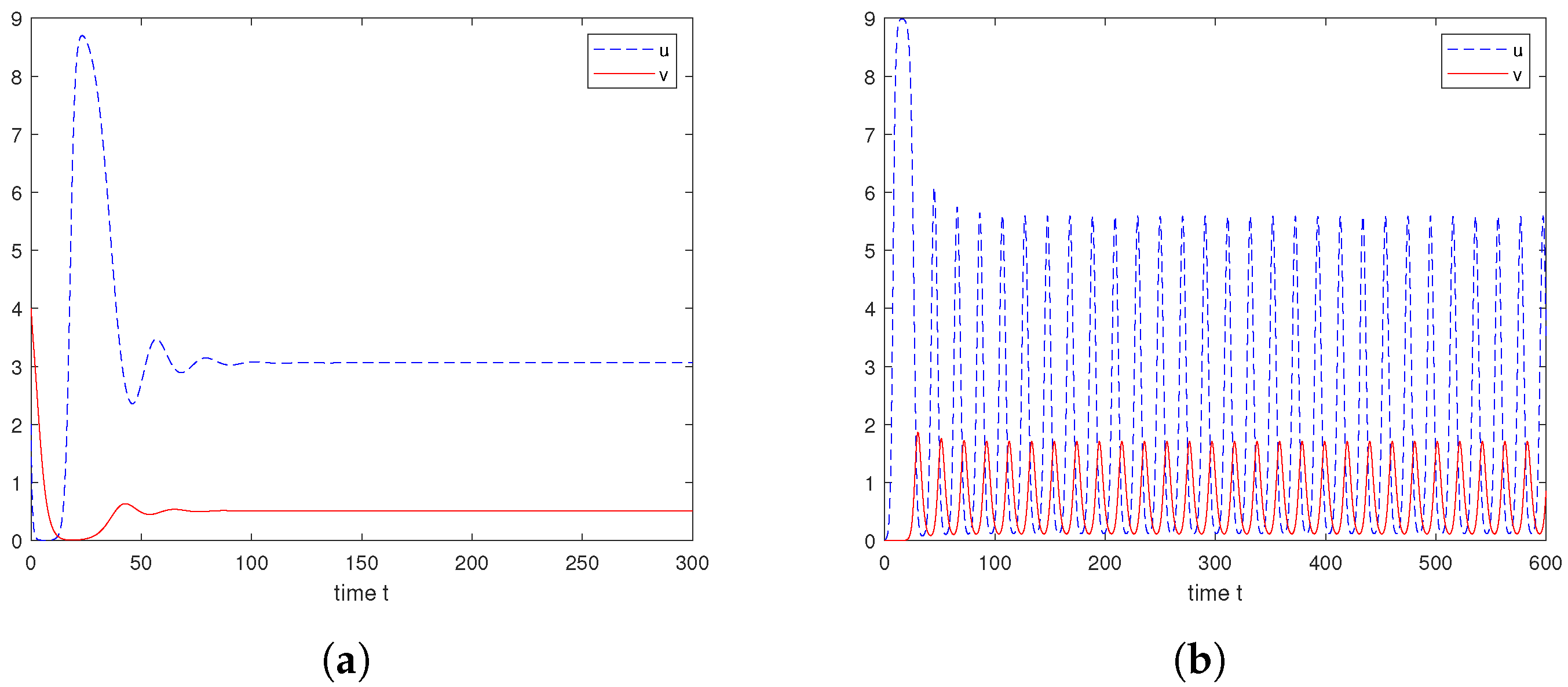
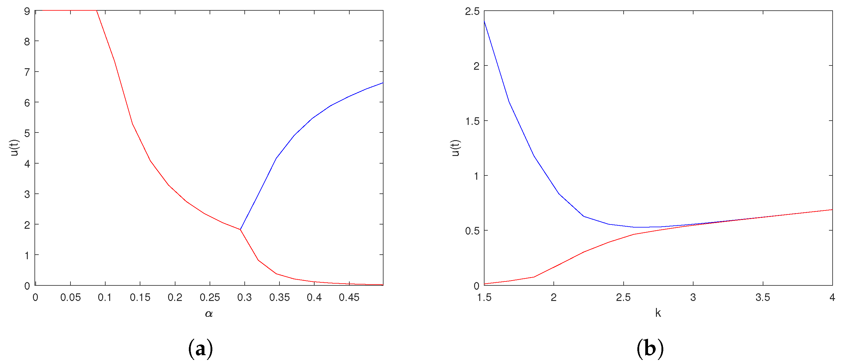
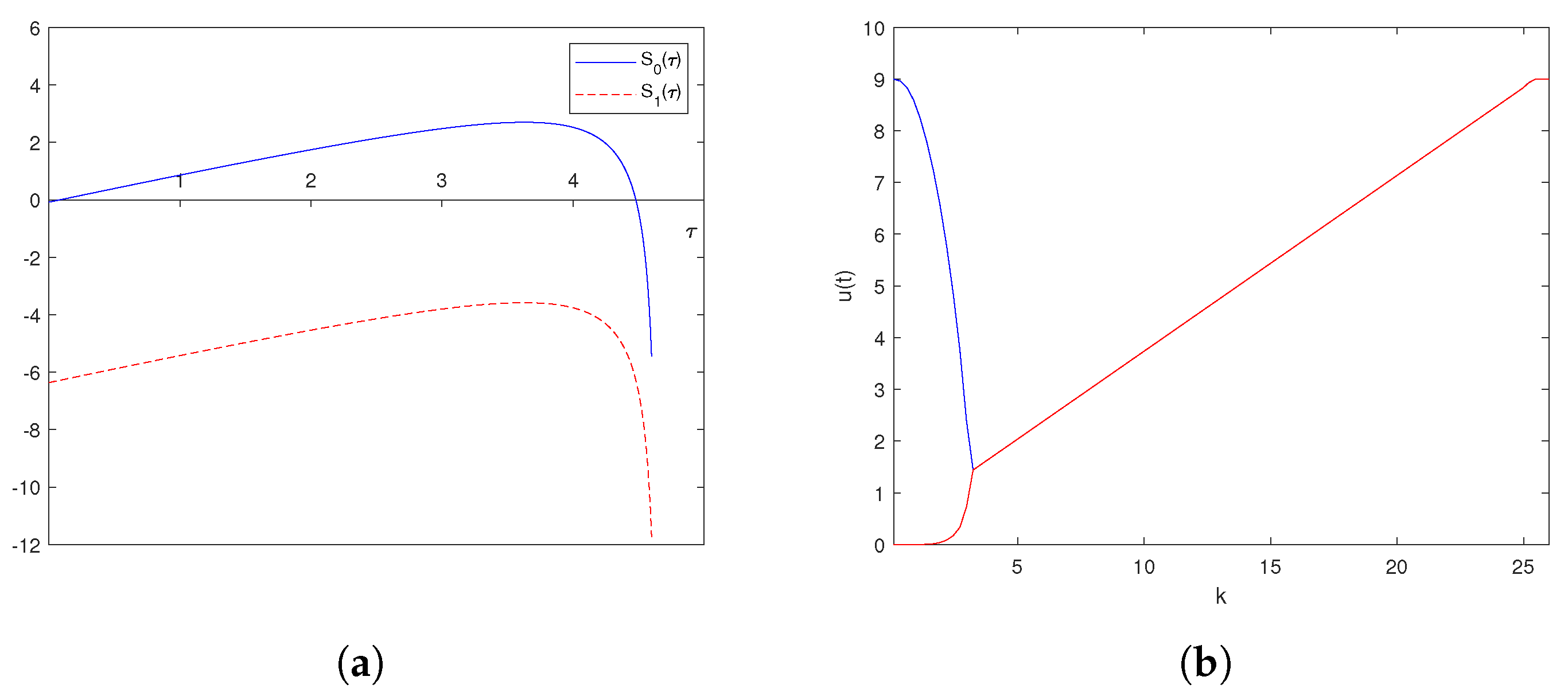
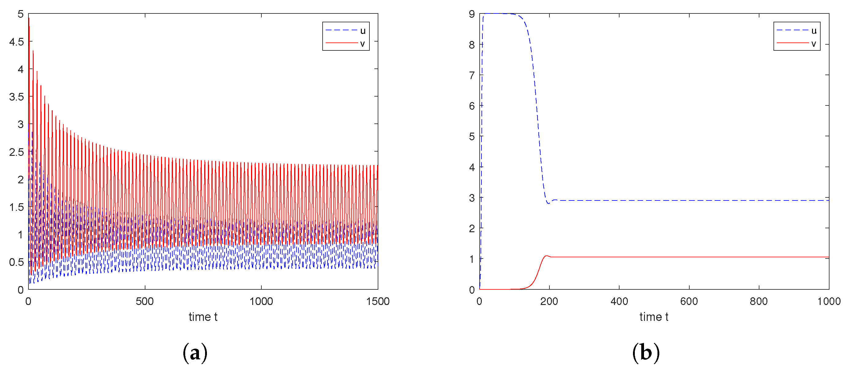
6. Numerical Explorations

As in Wang and Zou [7], we let $g(k,u)=\rho \left(k\right)u$, $\rho \left(k\right)={\displaystyle \frac{1}{1+c_{1}k}}$, and $f(k,v)={\displaystyle \frac{1}{1+c_{2}kv}}$. We take the parameter values as

$$r=1,c_1=1,c_2=1,d=0.1,a=0.1,c=4,m=0.5,$$

(30)

where $c_1=c_2=1$ are taken from [7], and the values of other parameters are biologically acceptable. All the simulations are carried out in MATLAB R2020b, which was produced by MathWorks, a company headquartered in Natick, Massachusetts, USA. The numerical method we use is the Euler method.

For the strong kernel case, we fix $\alpha =10$. Solving the equation $m=cg\left(k,{\displaystyle \frac{r-d}{a}}\right){\int }_0^{\infty }F\left(s\right)ds$ gives $k=64.3061$. If $k>64.3061$, Theorem 3 shows that $P_1=(9,0)$ is globally asymptotically stable (see Figure 1a for $k=65$). When $k<64.3061$, $P_1=(9,0)$ becomes unstable, and there is a unique coexistence equilibrium $P^{*}$. If we take $k=10$, then $P^{*}=(1.5159,0.263)$ and the inequality $A<u^{*}<{\displaystyle \frac{r-d}{a}}$ holds, and then, by Theorem 5, $P^{*}=(1.5159,0.263)$ is locally asymptotically stable (see Figure 1b).

If we let $k=1$, then solving $H_2\left(\alpha \right)=B_1\left(\alpha \right)B_2\left(\alpha \right)B_3\left(\alpha \right)-B_3^2\left(\alpha \right)-B_1^2\left(\alpha \right)B_4\left(\alpha \right)=0$, we obtain ${\alpha }_0=0.29$ and ${\displaystyle \frac{d{H}_2}{d\alpha }}{|}_{\alpha ={\alpha }_0}=-6.8539<0$, which means ${\displaystyle \frac{d\left(Re\lambda \right)}{d\alpha }}{|}_{\alpha ={\alpha }_0}>0$. When $\alpha$ passes through $0.29$, the coexistence equilibrium $P^{*}$ will loses its stability and periodic solutions will appear. As shown in Figure 2a and Figure 2b, we let $\alpha =0.2$ and $\alpha =0.4$, respectively, and these figures demonstrate that $\left(u\right(t),v(t\left)\right)$ switches from stable to periodic oscillation. Bifurcation diagrams in terms of $\alpha$ and k are depicted in Figure 3a and Figure 3b, respectively. Note that, for the strong kernel, the mean delay $\tau ={\displaystyle \frac{2}{\alpha }}$; thus, Figure 3a shows that a periodic solution occurs for a small $\tau$, and then the solution becomes stable as $\tau$ increases, where two populations coexist. Finally, the predator becomes extinct for a large $\tau$. As shown in Figure 3b, the system is unstable at first, which shows periodic oscillation, and when we increased the strength of the fear, we observed that the system became stable around the coexistence equilibrium. Therefore, high levels of fear can stabilize the steady state.

For the delta kernel, we let the parameter $\tau$ vary from $0.05$ to 5. The corresponding solution trajectories of System (1) are depicted in Figure 4. It can be found from Figure 4 that the coexistence equilibrium $P^{*}$ exists and is stable when $\tau =0.05$, and, as $\tau$ increases, periodic oscillations can occur with $\tau =2$, where the oscillations become damped when $\tau =5$, and $P^{*}$ can regain stability. For a large $\tau$, the predator species will die out. Figure 4 shows that stability switches can occur as the $\tau$ varies. As shown in Figure 5a, we give the relation between $S_0\left(\tau \right)$, $S_1\left(\tau \right)$, and $\tau$ for $\tau \in [0,4.6]$ and $k=1$. We find that $S_0\left(\tau \right)$ has two positive zeros: ${\tau }_1^{*}=0.083$ and ${\tau }_2^{*}=4.48$. At ${\tau }_1^{*}$ and ${\tau }_2^{*}$, stability switches occur, and $P^{*}$ is stable for $\tau \in [0,{\tau }_1^{*})\cup ({\tau }_2^{*},4.6]$. Then, it is unstable for $\tau \in ({\tau }_1^{*},{\tau }_2^{*})$. These results are in agreement with Figure 4. A bifurcation diagram with respect to parameter k is presented in Figure 5b. We point out that, in Wang and Zou [7] with a functional response of Holling type I, when $P^{*}$ exists, it is always unstable if $\tau$ is greater than some critical value. Since, for the weak kernel case with uniform distribution, their numerical simulations results are similar to the strong kernel and the delta kernel, respectively; as such, we omitted their numerical results.

If the functional response is Holling type II, i.e., $g(k,u)={\displaystyle \frac{pu}{(1+c_{1}k)(1+qu)}}$, then, by taking the delta delay kernel, for example, when $p=0.5$, $q=0.6$, we set $k=1$ and keep the other parameters as those in (30). Then, if $\tau =0$, there is a periodic solution (see Figure 6a), and the periodic solution disappears when $\tau$ increases to $1.5$ (see Figure 6b). A bifurcation diagram of $u\left(t\right)$ versus $\tau$ is depicted in Figure 7.

7. Discussion

In this work, we modify the existing predator–prey models with the fear effect by introducing distributed delay. We assumed that, if the prey is captured, the time required for biomass transfer from the prey to the predator is not fixed; instead, it follows some distribution. Then, we proposed a differential system with distributed delay, where the functional response is a relatively general function, which is increasing with respect to the prey.

For the model with a general kernel function, we proved its well posedness, such as the positivity and boundedness of solutions. We discussed the global stability of the extinction equilibrium $P_0$ and the predator-free equilibrium $P_1$, which is the uniform persistence of the system. More precisely, we showed that, if the birth rate of the prey is no greater than the death rate, then both species die out; conversely, if the coexistence equilibrium $P^{*}$ does not exist, then $P_1$ is globally stable, that is, only the prey survives if $P^{*}$ exists, $P_1$ loses stability, and the solutions persist.

If we assume that the functional response is Holling type I, then, for a general delay kernel, we obtained criteria for the local asymptotic stability of $P^{*}$. Due to the introduction of distributed delays, depending on the forms of delay kernels, the characteristic equation of the coexistence steady state $P^{*}$ may differ significantly. For the weak kernel and the strong kernel, the characteristic equations are polynomials, while it is a transcendental equation for the delta kernel or uniform distribution. For the weak kernel and the strong kernel, as $\alpha$ varies, it is demonstrated that $P^{*}$ will lose stability and a Hopf bifurcation occurs. For the delta kernel, we found that time delay $\tau$ can induce stability switches.

We performed numerical simulations for four particular distributions. For the weak kernel and the strong kernel, System (1) is stable for a small $\alpha$, but it becomes unstable for a bigger $\alpha$, where periodic orbits appear. For the delta delay distribution, System (1) displays rich dynamics, and it is found that intermediate delays will destabilize the coexistence equilibrium. However, small delays and large delays have a stabilizing effect. The dynamics of System (1) with a uniform distribution is similar to the delta distribution. For all the distributions that we considered, we showed that, for small values of fear level k, the system undergoes periodic oscillations, and, as k increases, the system gains stability. Biologically, this means that, if the level of the fear effect in prey is increased, then the populations of the prey and predator may have a state transition, i.e., from periodic oscillation to stability. The fear effects and delay kernels together affect the population dynamics of the model.

Our theoretical, as well as numerical, simulations results indicate that delays play important roles in the dynamics of the system. For a functional response of Holling type I without delay, if we further neglect the benefit of the fear effect, i.e., $g(k,u)=g\left(u\right)$, then System (1) reduces to an ordinary differential equation model that was proposed by Wang et al. [4], where periodic solutions do not appear. How the delay is incorporated into the model also impacts the dynamical behavior. If the delay is fixed as a constant, then System (1) becomes the System (8) shown in Wang and Zou [7] (except that our model has an extra delay dependent parameter $e^{-m\tau }$). In [7], when the coexistence equilibria exist, it is unstable for all $\tau >{\tau }_0$, namely large time delay always destabilize the system, which is opposite to our results. Figure 6 and Figure 7 indicate that different functional responses also have a significant impact on model dynamics.

An extension of our model that considers the impact of seasonality would be an interesting study. Incorporating the age structure or nonlinear harvesting of the predator is also another interesting topic. These problems will be left for further investigation. Our method may be applicable or useful to analyze the dynamics of other population models with distributed delays. Applying our method for population models with spatial heterogeneity and temporal dependence may lead to incorrect statements.

References

1. Creel, S.; Christianson, D.; Liley, S.; Winnie, J.A., Jr. Predation risk affects reproductive physiology and demography of elk. Science 2007, 315, 960. [Google Scholar] [CrossRef] [PubMed]
2. Suraci, J.P.; Clinchy, M.; Dill, L.M.; Roberts, D.; Zanette, L.Y. Fear of large carnivores causes a trophic cascade. Nat. Commun. 2016, 7, 10698. [Google Scholar] [CrossRef]
3. Zanette, L.Y.; White, A.F.; Allen, M.C.; Clinchy, M. Perceived predation risk reduces the number of offspring songbirds produce per year. Science 2011, 334, 1398–1401. [Google Scholar] [CrossRef]
4. Wang, X.; Zanette, L.; Zou, X. Modelling the fear effect in predator-prey interactions. J. Math. Biol. 2016, 73, 1179–1204. [Google Scholar] [CrossRef]
5. Holling, C.S. The functional response of predators to prey density and its role in mimicry and population regulation. Mem. Ent. Soc. Can. 1965, 97, 1–60. [Google Scholar] [CrossRef]
6. Wang, X.; Zou, X. Modeling the fear effect in predator-prey interactions with adaptive avoidance of predators. Bull. Math. Biol. 2017, 79, 1325–1359. [Google Scholar] [CrossRef] [PubMed]
7. Wang, Y.; Zou, X. On a predator-prey system with digestion delay and anti-predation strategy. J. Nonlinear Sci. 2020, 30, 1579–1605. [Google Scholar] [CrossRef]
8. Sasmal, S.K.; Takeuchi, Y. Dynamics of a predator-prey system with fear and group defense. J. Math. Anal. Appl. 2020, 481, 123471. [Google Scholar] [CrossRef]
9. Hossain, M.; Pal, N.; Samanta, S. Impact of fear on an eco-epidemiological model. Chaos Solitons Fractals 2020, 134, 109718. [Google Scholar] [CrossRef]
10. Mishra, S.; Upadhyay, R.K. Strategies for the existence of spatial patterns in predator-prey communities generated by cross-diffusion. Nonlinear Anal. Real World Appl. 2020, 51, 103018. [Google Scholar] [CrossRef]
11. Ma, T.; Meng, X. Global analysis and Hopf-bifurcation in a cross-diffusion prey-predator system with fear effect and predator cannibalism. Math. Biosic. Eng. 2022, 19, 6040–6071. [Google Scholar] [CrossRef]
12. Li, Y. Global steady-state bifurcation of a diffusive Leslie-Gower model with both-density-dependent fear effect. Commun. Nonlinear Sci. Numer. Simulat. 2025, 141, 108477. [Google Scholar] [CrossRef]
13. Cong, P.; Fan, M.; Zou, X. Dynamics of a three-species food chain model with fear effect. Commun. Nonlinear Sci. Numer. Simulat. 2021, 99, 105809. [Google Scholar] [CrossRef]
14. Li, A.; Zou, X. Evolution and adaptation of anti-predation response of prey in a two-patchy environment. Bull. Math. Biol. 2021, 83, 59. [Google Scholar] [CrossRef]
15. Panday, P.; Pal, N.; Samanta, S.; Tryjanowski, P.; Chattopadhyay, J. Dynamics of a stage-structured predator-prey model: Cost and benefit of fear-induced group defense. J. Theor. Biol. 2021, 528, 110846. [Google Scholar] [CrossRef]
16. Liu, C.; Chen, Y.; Yu, Y.; Wang, Z. Bifurcation and stability analysis of a new fractional-order prey-predator model with fear effects in toxic injections. Mathematics 2023, 11, 4367. [Google Scholar] [CrossRef]
17. Li, Y.; He, M.; Li, Z. Dynamics of a ratio-dependent Leslie-Gower predator-prey model with Allee effect and fear effect. Math. Comput. Simul. 2022, 201, 417–439. [Google Scholar] [CrossRef]
18. Teslya, A.; Wolkowicz, G.S.K. Dynamics of a predator-prey model with distributed delay to represent the conversion process or maturation. Differ. Equat. Dyn. Sys. 2023, 31, 613–649. [Google Scholar] [CrossRef]
19. Driver, R.D. Existence and stability of solutions of a delay-differential system. Arch. Ration. Mech. Anal. 1962, 10, 401–426. [Google Scholar] [CrossRef]
20. Lin, C.J.; Wang, L.; Wolkowicz, G.S.K. An alternative formulation for a distributed delayed logistic equation. Bull. Math. Biol. 2018, 80, 1713–1735. [Google Scholar] [CrossRef]
21. Yuan, Y.; Blair, J. Threshold dynamics in an SEIRS model with latency and temporary immunity. J. Math. Biol. 2014, 69, 875–904. [Google Scholar] [CrossRef] [PubMed]
22. Wolkowicz, G.S.K.; Xia, H.; Wu, J. Global dynamics of a chemostat competition model with distributed delay. J. Math. Biol. 1999, 38, 285–316. [Google Scholar] [CrossRef]
23. Gourley, S.A.; Ruan, S. Spatio-temporal delays in a nutrient-plankton model on a finite domain: Linear stability and bifurcations. Appl. Math. Comput. 2003, 145, 391–412. [Google Scholar] [CrossRef]
24. Deng, J.; Shu, H.; Wang, L.; Wang, X.S. Viral dynamics with immune responses: Effects of distributed delays and Filippov antiretroviral therapy. J. Math. Biol. 2023, 86, 37. [Google Scholar] [CrossRef] [PubMed]
25. Shu, H.; Chen, Y.; Wang, L. Impacts of the cell-free and cell-to-cell infection modes on viral dynamics. J. Dyn. Diff. Equat. 2018, 30, 1817–1836. [Google Scholar] [CrossRef]
26. Beretta, E.; Kuang, Y. Geometric stability switch criteria in delay differential systems with delay dependent parameters. SIAM J. Math. Anal. 2002, 33, 1144–1165. [Google Scholar] [CrossRef]
Figure 1. The solution trajectories of System (1), with α = 10 , in the strong kernel case. (a) For k = 65 , the prey persists but the predator dies out. The initial condition is as follows: ( u ( θ ) , v ( θ ) ) = ( 2 , 4 ) for θ ( , 0 ] . (b) When k = 10 , both species persist, and they will then stabilize in a stable level. The initial condition is as follows: ( u ( θ ) , v ( θ ) ) = ( 2 , 4 ) for θ ( , 0 ] .
Symmetry 17 00604 g001
Figure 2. The solution trajectories of System (1), with k = 1 , in the strong kernel case. (a) For α = 0.2 , the coexistence equilibrium was stable. The initial condition is as follows: ( u ( θ ) , v ( θ ) ) = ( 2 , 4 ) for θ ( , 0 ] . (b) When α = 0.4 , a periodic solution occurs. The initial condition is as follows: ( u ( θ ) , v ( θ ) ) = ( 0.01 , 0.001 ) for θ ( , 0 ] .
Symmetry 17 00604 g002
Figure 3. Bifurcation diagram of the prey versus α and k in the strong kernel case. (a) The prey species can be understood as a function of α when k = 1 and α varies from 0.01 to 0.5. (b) The prey species can be understood as a function of k when α = 10 and k varies from 1.5 to 4.
Symmetry 17 00604 g003
Figure 4. The solution trajectories of System (1) in the delta kernel case when τ varies. (a) τ = 0.05 . The initial condition is as follows: ( u ( θ ) , v ( θ ) ) = ( 0.05 , 0.01 ) for θ [ 0.05 , 0 ] . (b) τ = 2 . The initial condition is as follows: ( u ( θ ) , v ( θ ) ) = ( 0.05 , 0.01 ) for θ [ 2 , 0 ] . (c) τ = 5 . The initial condition is as follows: ( u ( θ ) , v ( θ ) ) = ( 0.05 , 0.01 ) for θ [ 5 , 0 ] .
Symmetry 17 00604 g004
Figure 5. Graphs of the stability switch in terms of time delay τ and k in the delta kernel case. (a) Graphs of S 0 ( τ ) and S 1 ( τ ) . Here, k = 1 and τ vary from 0 to 4.6. (b) The prey species as a function of k. Here, τ = 2 and k varies from 0 to 26.
Symmetry 17 00604 g005
Figure 6. The solution trajectories of System (1) for a functional response of Holling type II. (a) τ = 0 . The initial condition is as follows: ( u ( 0 ) , v ( 0 ) ) = ( 0.05 , 0.01 ) . (b) τ = 1.5 . The initial condition is as follows: ( u ( θ ) , v ( θ ) ) = ( 0.05 , 0.01 ) for θ [ 1.5 , 0 ] .
Symmetry 17 00604 g006
Figure 7. A bifurcation diagram of the prey versus τ for a functional response of Holling type II. Here, k = 1 and τ varies from 0 to 2.5. All the other parameter values are given in (30).
Symmetry 17 00604 g007
Disclaimer/Publisher’s Note: The statements, opinions and data contained in all publications are solely those of the individual author(s) and contributor(s) and not of MDPI and/or the editor(s). MDPI and/or the editor(s) disclaim responsibility for any injury to people or property resulting from any ideas, methods, instructions or products referred to in the content.