Abstract
This study aimed to examine changes in the number of live and dying trees in central Lithuanian forests over time. Results were obtained using stochastic differential equations combined with the normal copula function. The examination of each tree’s individual size variables (height and diameter) showed that the mean values of dead or dying trees’ size variables had significantly lower trajectories that were particularly pronounced in mature stands. According to the data set under examination, the tree mortality rate gradually declined with age, reaching approximately 7% after 10 years. Birch trees 60–70 years old were the first species to reach the 1% mortality rate, followed by spruce trees 70–80 years old and pine trees 80–90 years old. The Maple symbolic algebra system was used to implement all results.
1. Introduction
Theories that suggested a decline in resource usage efficiency and received significant support in the past were not accurately formalized mathematically. Much of that research was undertaken to determine the importance of specific tree size variables when analyzing the mortality rate in a forest stand that is not influenced by environmental perturbations [1]. Forest statisticians studied the equilibrium between a stand’s tree sizes and stocking density. The fundamental idea discussed in modeling literature is that there is a relationship between the balance of mortality, stocking density, and stand growth after a forest stand’s mortality has reached a plateau [2]. The main goal of this study was to provide a quantitative evaluation of changes in live and dying tree numbers over time (not static) according to different tree species in mixed-species and uneven-aged stands. A key factor driving changes in stands’ spatial heterogeneity is the tree mortality phenomenon. When a stand is first established, thousands of seedlings are planted per hectare, and the evolution of unmanaged stands demonstrates that most trees in a stand naturally die due to competition [1,2]. The literature provides an extensive overview of the rates and causes of mortality at various stages of stand evolution; however, little research has addressed the dynamics of the number of dead or dying trees or how this process changes with age [1,3,4]. Assessing tree mortality factors and dynamics is among the most essential aspects of the proper use, conservation, and restoration of forest ecosystems. In boreal forests, tree mortality is mainly influenced by competition, age, disease, and random changes in the forest environment. In the early phases of forest development, competition is especially intense as young trees fiercely compete for water, nutrients, and sunlight [5]. This study refers to dying and dead trees in a stand as forming the same class. Standing dead trees, which can take a long time to die, and fallen trees are both sources of clusters of dying trees. Even with the far-reaching effects of dead wood accumulation, our quantitative understanding of trees’ ongoing mortality and the reduction in wood volume over longer periods is quite limited. As the value of the tree-level size variable in a stand and the demand for resources to support the growth process both increase, competition between neighboring trees arises, resulting in two processes occurring simultaneously: the process of each individual tree’s natural mortality and the growth process of living tree size variables. The regular loss of trees due to mortality means that a stand’s biomass at a particular age consists of the biomass of growing trees and dying trees. The forecasted mortality time of a particular tree depends on many fixed and random environmental factors, including location, species composition, air quality, and climate. The most common statistical model used to study individual tree and stand mortality is the logistic regression model. Annual survival logistic regression equations predict the probability that a tree will survive the following year. Consequently, it might be challenging to calculate annual survival probability using data that are routinely obtained at intervals longer than a year. The process-driven model presented in this study is dynamic and can be fitted with remeasurements in cycles of unequal periods. Age and tree-level size variables (diameter, height, crown base height, etc.) are the main drivers of tree mortality in a stand, making tree mortality a dynamic phenomenon [6,7,8].
Individual tree mortality occurs when a tree is recorded as dead, but it is not possible to determine the exact time and cause of death. A precise mathematical definition of the dynamic process of mortality in a forest stand requires repeated measurements of experimental plots, which are usually not large enough. Most models that explain forest mortality dynamics rely on databases that combine dendrochronologically derived information on individual tree age and radial growth with static data on the forest’s structure and composition [9,10,11]. The dynamics of a region’s forests can be characterized using tree mortality rates.
For the past 20 years, experimental plots have served as the foundation for the majority of ecosystem-scale studies on tree mortality in stands [12,13]. Long-term tree mortality trajectories would undoubtedly greatly improve our understanding of growth processes and increase our capacity for predicting stand development. However, long-term stand monitoring is expensive and time-consuming, which raises the problem of how to replace regression models used to simulate growth processes with more complex models that cover the whole age range of tree growth. Normal distribution with constant variance has long been central to building regression models for a wide range of values of modeled variables, but unfortunately, regression concepts are often applied to highly asymmetrical data [14,15,16].
This study proposed a dynamic model in all respects, defined by mixed-effects parameters and stochastic differential equations with unknown parameters estimated from repeated measurements on permanent experimental plots. Most current models of the mortality process are based on even-aged forest conditions, as they assume that mortality is simply calculated as the ratio of the mean annual mortality to the number of trees per hectare and requires uniform intervals of the remeasurement cycle throughout the time interval. These models, therefore, have two main limitations: (1) they may distort the actual underlying process, as it is continuous in time, which may lead to the misidentification of relationships, and (2) they have difficulty adjusting to non-uniform intervals in remeasurement cycles. Without a doubt, many phenomena that have been continually observed throughout time in domains like forestry, biology, and ecology have inherent uncertainty [17,18,19,20]. Stochastic differential equation models outperform deterministic models in these situations because they relate to stochastic processes that can capture both the unpredictability of the underlying trajectory and the deterministic trend [21,22]. Typically, random noise drives stochastic differential equations and is represented by the standard Brownian process [23,24]. Using Brownian motion to control a stochastic differential equation’s trajectory is mathematically supported by the central limit theorem, which states that normal distribution is naturally found in “many” situations, namely as a case of a limit distribution. Therefore, to model biological processes without sufficient information about the shape of the probability distribution of the quantity being modeled, it is appropriate to define changes in the quantity over time using a stochastic differential equation constructed using a normal distribution [25]. Stochastic differential equations with fixed- and random-effect parameters have been used to predict tree-size components (diameter at breast height, height, crown base height, volume, etc.) using univariate or multivariate measurements. Because the modeled variable was dynamic, it was possible to analyze the dynamics of the current size increment as well as tree-level size variables in detail using models defined by stochastic differential equations [26,27]. For a long time, forest statisticians focused on modeling individual tree size variables (diameter, height, etc.) using sigmoidal regression models, as changes in plant development over time follow a sigmoidal pattern [28].
The development of model systems that describe the growth behavior of trees and stands has yielded a significant amount of knowledge. Fluctuations in the number of living and dying trees in a stand over time are described herein, taking into account the process-driven method’s superiority and focusing on earlier research regarding stochastic differential equations and copula functions. This approach is superior to commonly applied static regression methods. Notably, in the past, the number of living trees was traditionally determined using the balancing regression equation between a stand’s stocking density and tree sizes.
2. Methodology
The main goal of this study was to define the linkage between a tree’s potentially occupied area and tree mortality processes to characterize more precisely the dynamics of the number of dead and living trees per hectare. Two methods were used in this study: (1) the dynamic of the individual tree size variable was described in the diffusion process’ framework, and the corresponding exact transition probability density function was obtained; (2) density functions of individual tree size variables were combined using the normal copula function. In this paper, we present a mixed-effects 4-parameter Gompertz-type stochastic differential equation to define the dynamics of tree size variables. Fixed- and random-effect parameters were estimated using an approximate maximum likelihood procedure and an observed estimation dataset. The number of living and dead trees per hectare and their relationship to the mean tree diameter and occupied area in a stand were examined. Results are illustrated visually and statistically and were implemented using the Maple symbolic algebra system.
This paper presents a simulation framework for the tree mortality process in a forest stand using stochastic differential equations (SDEs) and the normal copula function. The number of living and dead trees per hectare and their relationship to a stand’s mean diameter and height are examined. Transition probability density functions are derived in the exact form using the proposed mixed-effects parameters SDE framework, and parameter estimators for the diameter and occupied area are produced using an approximated maximum likelihood technique. In the next step, we estimate the dependence parameter of the two-dimensional copula density function. Finally, we define the number of live trees in the stand as the mean value of the random variable using the integration operation, as all densities with the corresponding parameter estimates are known, and using the derivative operation, we define the number of dying trees in the stand. This formalization also makes it possible to write formulas for volume and basal area calculations using an integration process, which may support foresters in assessing various management strategies. The framework was designed to make it as flexible as possible by allowing machine-learning resources to adapt in response to evolving conditions at any point, as depicted in Figure 1.
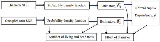
Figure 1.
SDE algorithm flow chart visualization.
2.1. Stochastic Differential Equation Framework
The probability distribution of tree-level size variables is useful for defining the mean, mode, median, quantiles, and other numerical characteristics of tree-level and stand-level size attributes. The main tools for assessing tree or stand quantitative and qualitative characteristics are tree height and diameter distributions [29,30]. Classical, well-known distributions, including gamma, Weibull, normal, exponential, and others, are most frequently used by forest statisticians [31,32]. The main drawback of these distribution models is that they are not associated with trees’ ages. Itô-type [23,33] stochastic differential equations, which describe diffusion processes, can be effectively used to determine the relationship between changes in a tree size variable and a tree’s age or a stand’s average age.
Vasicek, Gompertz, Bertalanffy, and gamma SDE growth models provide exact solution transition probability density functions. In this paper, we use a multiplicative form of noise and a one-dimensional mixed-effects 4-parameter Gompertz-type stochastic differential equation, separately defining the dynamics of the area occupied by the tree and those of the tree’s diameter. Suppose that change rates in tree diameter at breast height , i = 1, …, M; k = 1, …, ni1 (M is the number of plots and ni1 is the number of trees in the ith plot), and change rates in the occupied area are determined according to the Gompertz-type stochastic differential equation:
where and are birth rate parameters, and are death rate parameters (, > 0 and , > 0), are threshold parameters, are volatility coefficients, and random effects , , i = 1, …, M have constant variances and zero means. They are independent, normally distributed random variables, respectively, and . Moreover, is a random variable that is independent to and an initial condition takes the following form: if t = t0, then , and The unknown fixed-effect parameters vectors = {, , , } and = {, , , } must be estimated.
After performing the process transformation , j = 1, 2, we can derive the transition probability density function of the solution in the exact form. The solution of the 4-parameter Gompertz-type stochastic differential Equation (1) has a lognormal distribution , i = 1, …, M, with the mean , the variance , j = 1, 2; k = 1, …, nij, and the probability density function , as follows:
The dynamics of the mean, median, , mode, , qth quantile (0 < q < 1), , and variance, , i = 1, …, M, of the diameter are given by the following expressions:
2.2. Bivariate Normal Copula
Copula functions play an important role in linking one-dimensional probability distributions to multidimensional distributions of a particular form. That parameter estimates of tree diameter and occupied area stochastic differential Equation (1) may be obtained utilizing different samples highlights the benefit of employing the copula function method. Sklar’s theorem makes this link possible [34]. The normal copula function has attracted particular attention because the normal probability distribution is widely used in agriculture, biology, engineering, economics, and finance. Let us define a normal two-dimensional copula function. The two-dimensional normal copula distribution function with correlation parameter is defined using Sklar’s formula in the following form:
where
The two-dimensional normal copula probability density function takes the following form:
where and . The joint two-dimensional copula-type probability density function is given as follows:
where and , j = 1, 2 are the probability density and cumulative distribution functions of Xj, respectively.
The conditional probability density function of , j = 1, 2 at a given , j ≠ k, is defined as follows:
2.3. Semiparametric Maximum Pseudo-Likelihood Procedure
Given that in the previous section we determined the exact transition probability density functions for tree diameter and occupied area and the two-dimensional normal copula function that connects them, we can directly apply the maximum likelihood method to estimate unknown parameters. The direct implementation of the one-step maximum likelihood method raises several numerical problems in optimizing the maximum log-likelihood function [35]. Naturally, estimating parameters using the maximum log-likelihood function can be divided into two steps.
In the first step, Equations (1) and (2) can be fitted to the diameter sample dataset or occupied area sample dataset at discrete times (ages) (nij is the number of observed trees of the ith plot for the jth variable, i = 1, 2, …, M) using the maximum likelihood procedure. The associated maximum log-likelihood function for the mixed-effects parameters takes the following form:
where are fixed-effect parameters (the same for all plots), the normal density function of random effects is , and .
For mixed-effects parameters Models (1) and (2), the two-stage approximated maximum log-likelihood procedure takes the following form (j = 1, 2; i = 1, …, M):
where
and argmax is an operation that finds the argument that gives the maximum value from a target function.
The maximization of is a two-stage optimization problem. The internal optimization step estimates the for every plot i = 1, …, M using Equation (18). The external optimization step maximizes after plugging , i = 1, …, M into Equation (17).
In the second step, we estimate the density parameters of the two-dimensional copula density function defined using Equation (13) by maximizing the log-likelihood copula function defined as follows:
where and is the inverse of a standard normal distribution.
2.4. Parameter Calibration
The main challenge in defining the dynamics of tree size variables comes from calibrating random effects to the new stand. Observed data from a new plot were used in this study to estimate random effects [36]. If there are no measurements of standing dead trees in a new plot, the random effects needed to define the dynamics of the dead tree size variables are equated to the corresponding random effects of the living trees. For a new plot, the random effects are defined in the following form [37]:
where the number of observed trees in a plot is denoted by m, , j = 1, 2 (tree diameter or occupied area) is the newly observed dataset (measured plot) on fixed time values , t0 = 4, and is the log-normal density function defined using Equation (5). Estimated values of fixed-effect parameters for mixed-effects Models (1) and (2) are denoted by “hat” and are estimated separately for living and dead trees using an approximated maximum likelihood procedure described using Equations (17)–(19).
3. Material
3.1. Sample Collection
In this paper, we present 37 years of measurements from continued monitoring of permanent experimental plots. During the 1983–1987 period, 53 permanent experimental plots were installed in the forests of Lithuania’s Kazlų Rūda region and measured between one and seven times at 2- to 37-year intervals. Figure A1 shows the location of the permanent experimental plots in the forests of the Kazlų Rūda region of Lithuania. The sampling method used rectangular plots that consisted of about 0.16–0.72 ha. The area covered by Scots pine (Pinus sylvestris L.) stands accounts for 63.8% of the particular allocation; Norway spruce (Picea abies) for 30.2%; silver birch (Betula pendula Roth and Betula pubescens Ehrh.) for 5.8%; and other stands for 0.2%. From 1983 to 2020, 58,829 live trees (36,689 pine, 18,738 spruce, 3270 birch, and 132 other species) were measured in 48 plots. During each measurement, the following were recorded for every sample tree: age, diameter at breast height, and tree position (x and y coordinates). The area occupied by a tree was determined by measuring each tree’s location inside the plots and utilizing a Voronoi diagram [37]. Trees that fell out of measurement within 37 years were considered dead. Figure 2 shows the dynamics of the number of trees per ha depending on the stand’s average age by tree species. A total of 16,857 trees (10,620 pine, 5049 spruce, 1104 birch, and 94 others) died in 48 plots from 1983 to 2020, which represents 28.7% of the sample population (58,829 trees). In most cases, we were unable to identify the causal agent, and death was not consistently associated with biotic or abiotic forest characteristics.

Figure 2.
Dynamics of the number of observed trees per hectare: (a) all species; (b) Scots pine; (c) Norway spruce; and (d) silver birch.
Notably, the data-gathering process design likely contributed to the uncertainty of model predictions. Most likely, number-of-trees-per-hectare models lacked precision because age was a complicated variable to control in these ongoing experiments. This was problematic, as only 10% of trees whose height was measured had their age measured; the remaining trees were evaluated based on an average age.
3.2. Parameter Estimation
We used the semiparametric maximum likelihood method described above to find unknown parameters, where the diameter of the trees and the area occupied by the trees at a fixed point in time were discretely measured for i = 1, …, M in M = 48 plots. Parameters of the stochastic differential Equation (1) were estimated separately for living and dead (dying) trees under four possible outcomes: all trees, Scots pine, Norway spruce, and silver birch. The results of the parameter estimation are summarized in Table 1. All parameters were statistically significant. The observed Fisher information matrix, which is the negative of the second derivative (the Hessian matrix) of the approximated maximum log-likelihood function, was used to estimate standard deviations [38].

Table 1.
Parameter estimates for Equations (1) and (2) for living and dead trees.
Equation (20) was used to estimate the parameter of dependence, , which yielded values of 0.2913 for all tree species, 0.2180 for pine, 0.2374 for spruce, and 0.1999 for birch.
4. Results and Discussion
4.1. Effect of Age on Mortality
Deadwood is generally classified according to its position in relation to the forest canopy as standing or fallen because the decay rate of standing deadwood can be much lower than that of fallen deadwood. In this study, each stand’s standing and fallen dead trees were merged into a single class called dead (dying) trees. As trees age, stands naturally change into a phase of spontaneous decline in stem number in a process known as self-thinning. In forestry research, a complicated phenomenon like tree self-thinning is typically described mathematically as a power function between the number of trees per hectare (stand density) and tree size (e.g., mean diameter, volume, or biomass) [39,40,41]. This proposed power function is universal but dependent on species, age, and environmental conditions. Subsequent investigations by Yoda [3] and Mrad et al. [42] documented similar patterns relating to the time dependency of tree size and density. Modeling forest growth requires self-thinning equations to predict changes in stand density by tree species, age, and any combination of species or age. Using the stochastic differential Equation (1) for the dynamics of a tree’s occupied area (j = 2), we defined the dynamics of the number of trees per ha for four outcomes: all tree species, pine species, spruce species, and birch species in a forest stand using the following equation:
where estimates of fixed-effect parameters are from living trees data in Table 1; and random effects are calibrated using Equation (21) or, in the case of a fixed-effect scenario, are set to the mean values, namely zero ().
We defined the dynamics of the number of trees per hectare of dead trees using the derivative operation, as follows:
where estimates of fixed-effect parameters are taken from living trees data in Table 1; and random effects are calibrated using Equation (21) or, in the case of a fixed-effect scenario, are set to the mean values, namely zero ().
Tree mortality per hectare is often defined differently [43,44], so it makes sense to have a single measure of mortality. The absolute mortality rate per hectare derived from Equation (23) depends on the existing number of trees in the stand and is therefore not useful for mortality analysis when comparing stands with different initial numbers of trees. In this case, the relative mortality rate, or, in other words, the instantaneous dynamics of the relative mortality rate, is defined as the decrease in the number of trees per hectare compared to the current number of trees (using a percentage scale) in the following form:
The relationship between relative mortality and logarithmic size characteristics, expressed in Equation (24), is commonly used in forestry, for example, to describe the relationship between the number of trees per hectare in a stand and tree size [25,45,46].
Figure 3 shows simulated trajectories of the number of trees per hectare of living and dead trees, along with observations, and dynamics of tree mortality in the stand are shown on a percentage scale. Figure 3a–c shows that thinning occurred at a high rate in stands up to 60 years of age, whereas in stands above 90 years of age, the rate was below 1%. Figure 3 also shows trends in the number of living and dead trees per ha in all mixed-species, uneven-aged stands in the region, ignoring the plot’s characteristics (only fixed-effect parameters were used). Figure 4 visualizes analogous trajectories for Scots pine, Norway spruce, and silver birch species separately. In this region, Norway spruce had significantly lower relative mortality than other tree species, as seen by comparing Figure 4(p3,s3,b3).
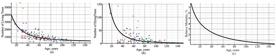
Figure 3.
Trajectories of number of trees per 1 ha: (a) living trees; (b) dead trees; (c) dead–living trees ratio expressed as a percentage. Circles indicate observed values.
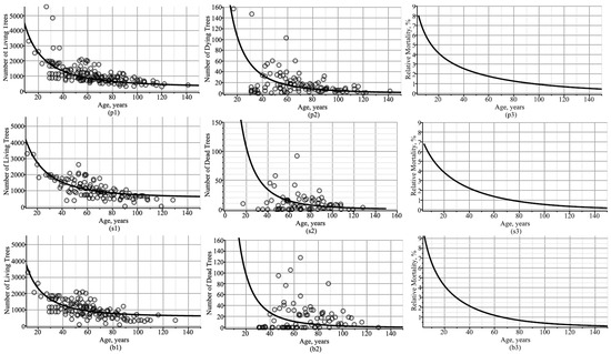
Figure 4.
Trajectories of number of trees per 1 ha: (p1,s1,b1) living trees; (p2,s2,b2) dead trees; (p3,s3,b3) dead–living trees ratio expressed as a percentage; (p1,p2,p3) pine species; (s1,s2,s3) spruce species; (b1,b2,b3) birch species. Circles indicate observed values.
4.2. Effect of Tree Size on Mortality
Next, we analyze how the mean diameter of trees in a stand affects the number of trees per ha. To determine the conditional number of trees per hectare in relation to the mean diameter of trees in the stand, we use a copula-type two-dimensional probability density function of the tree diameter and the occupied area, which is defined using Equation (14) and an additional integration operation, as follows:
where conditional probability density function is defined as:
and = ; j = 1, 2; estimates of fixed-effect parameters are taken from living trees data in Table 1; the parameter of dependence is estimated using Equation (21) (for all tree species, 0.2913; for pine, 0.2180; for spruce, 0.2374; and for birch 0.1999); and random effects are calibrated using Equation (21) or, in the case of a fixed-effect scenario, are set to the mean values, namely zero ().
Next, we visually analyze whether the number of trees per hectare is affected by the mean diameter of a forest stand. For Figure 5, the number of trees per hectare was modeled by taking three different trajectories of tree diameter dynamics: the mean (defined using Equation (6)), the 5% quantile, and the 95% quantile (defined using Equation (9)). Figure 5 shows that a strong increase in the diameter trajectory significantly affected the dynamics of the number of trees per ha. In this context, it is appropriate to investigate the rates of increase and decrease in the number of trees per ha as a function of the rate of change in the trajectory of tree diameter in a forest stand. For this purpose, the mean tree diameter in the stand, as defined using Equation (6), was increased or decreased by 10%, 25%, and 50%, and the effect on the number of trees per ha is shown graphically in Figure 6. Increasing the mean stand diameter by 10%, 25%, and 50% would reduce the number of trees per hectare by more than 3.5%, 8%, and 14%, respectively, at an average stand age of 60 years (see Figure 6a). On the other hand, reducing the mean stand diameter by 10%, 25%, and 50% would increase the number of trees per hectare by more than 4%, 10%, and 24%, respectively, at an average stand age of 60 years (see Figure 6b). This confirms that thinning accelerates the increase in stand diameter and reduces the number of trees in the stand.
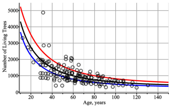
Figure 5.
Dynamics of the number of trees per ha of living trees using different trajectories of tree diameter in a stand: mean diameter trend (black); the trend of the diameter’s 5% quantile (red); the trend of the diameter’s 95% quantile (blue). Circles indicate the observed dataset.
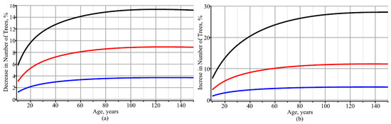
Figure 6.
Percentage dynamics of decreases or increases in the number of trees per hectare: (a) mean increases in diameters of the stand’s trees of 10% (blue), 25% (red), and 50% (black); (b) mean decreases in diameters of the stand’s trees of 10% (blue), 25% (red), and 50% (black).
The analysis of the number of trees per hectare shown in Figure 4, Figure 5 and Figure 6 was carried out using a fixed-effect scenario, i.e., random effects were equated to their mean values, which were zero under the previous assumption. The analysis of the dynamic of the number of trees per hectare under the mixed-effects scenario is presented below. For this purpose, estimates of fixed-effect parameters were taken from Table 1, and random effects were calibrated according to Equation (21). Figure 7 shows the dynamic of the number of trees per ha for living and dead trees and the dynamic of the relative mortality (dead–live trees ratio). Simulated trajectories of the number of trees per ha for all species of trees were in good agreement with the observed values for both living and dead trees, as shown in Figure 7(a1,p1,s1,b1) (for living trees) and Figure 7(a2,p2,s2,b2) (for dead trees). Notably, the tree mortality rate reached about 7% from the age of 10 years onwards and steadily decreased with age (see Figure 7(a3,p3,s3,b3)). Figure 7(a3,p3,s3,b3) shows that birch species (60–70 years old) reached the 1% mortality rate the fastest, followed by spruce species (70–80 years old) and then pine species (80–90 years old). In the case of pine species, the proportion of species in the species composition did not affect the mortality rate (see Figure 7(p3)). In contrast, birch species showed a higher mortality rate with a low proportion of birch species (see Figure 7(b3)).
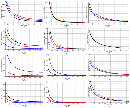
Figure 7.
Trajectories of the number of trees per 1 ha for the mixed-effects scenario: (a1,a2,a3) all species of trees: the first stand consisted of 92% pine (P), 2% spruce (S), and 6% birch (B) (black), the second stand consisted of 14% P, 82% S, and 4% B (red), and the third stand consisted of 60% P, 3% S, and 37% B (blue); (p1,p2,p3) pine trees: the first stand consisted of 99% P, 0% S, and 1% B (black), the second stand consisted of 65% P, 31% S, and 4% B (red), and the third stand consisted of 18% P, 80% S, and 2% B (blue); (s1,s2,s3) spruce trees: the first stand consisted of 18% P, 80% S, and 2% B (black), the second stand consisted of 49% P, 48% S, and 3% B (red), and the third stand consisted of 60% P, 3% S, and 37% B (blue); (b1,b2,b3) birch trees: the first stand consisted of 37% P, 26% S, and 37% B (black), the second stand consisted of 84% P, 0% S, and 16% B (red), and the third stand consisted of 92% P, 2% S, and 6% B (blue); (a1,p1,s1,b1) living trees; (a2,p2,s2,b2) dead trees; (a3,p3,s3,b3) dead–living trees ratio, expressed as a percentage. Circles indicate observed values.
To understand the mechanisms underlying tree mortality, it is worthwhile to investigate further the relationship between stand size attributes (mean diameter, height, etc.) and the relative mortality between different tree species and environmental conditions. To find a link between relative mortality and mean size attributes, we used tree diameter, height, and occupied area as size proxies and investigated their relationship with relative mortality. It has been repeatedly observed in the literature that mortality rates have a general multivariate dependence on tree size attributes and various environmental factors [4,47]. The analysis of the dynamic of relative mortality’s dependence on mean diameter and mean occupied area, shown in Figure 8, was carried out using a fixed-effect scenario; i.e., random effects were set to their mean values, which were assumed to be zero according to the previous assumption, estimates of fixed-effect parameters in Table 1 (living trees) were taken into account, and the mean trajectories of diameter and occupied area were calculated using Equation (5).
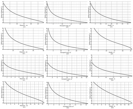
Figure 8.
Dead–living trees ratios, expressed as percentages, for the fixed-effect scenario: (a1,a2,a3) all species of trees; (p1,p2,p3) pine species; (s1,s2,s3) spruce species; (b1,b2,b3) birch species; (a1,p1,s1,b1) dynamic of dead–living trees ratio versus mean diameter; (a2,p2,s2,b2) dynamic of dead–living trees ratio versus mean occupied area; and (a3,p3,s3,b3) dynamic of dead–living trees ratio versus mean height.
As Figure 8 shows, Norway spruce’s relative mortality was the most likely to reduce, by up to 4%, when the mean diameter exceeded 1.5 cm or the occupied area exceeded 3 m2. In addition, Norway spruce’s relative mortality was reduced by up to 2% when the mean diameter exceeded 8 cm or the occupied area exceeded 6.5 m2. The next most common species in terms of the rate of decline in relative mortality was silver birch, for which the relative mortality rate decreased by up to 4% when the mean diameter was greater than 8 cm or the occupied area was greater than 4.5 m2. The relative mortality of silver birch decreased by up to 2% when the mean diameter exceeded 15 cm or when the occupied area exceeded 8 m2. The smallest decreases in relative mortality were observed for Scots pine: 4% relative mortality occurred when the mean diameter exceeded 9 cm or the occupied area exceeded 4.5 m2, and 2% relative mortality occurred when the mean diameter exceeded 19.5 cm or the occupied area exceeded 10 m2.
Relative mortalities shown in Figure 8 reflect all stands in the Kazlų Rūda region and do not take into account the peculiarities of tree growth processes in a particular stand. To reflect the effects of individual stands on differences in relative mortality required a mixed-effects scenario to be applied. Figure 9 shows the relationship of relative mortality with the mean tree diameter and the mean area occupied in three different stands. Figure 9 also shows the dependence of the relative mortality dynamic on the mean diameter and the mean occupied area under a mixed-effects scenario; i.e., random effects were calibrated according to Equation (21), fixed-effect parameters from Table 1 (living trees) were used, and the mean trajectories of diameter, height, and occupied area were calculated according to Equation (5). The asymptotic values of mean diameter and mean occupied area for pine species are roughly illustrated in Figure 9: e.g., mean diameters were 32 cm (black in the first plot), 42 cm (red in the second plot), and 49 cm (blue in the third plot); and mean occupied areas were 23 m2 (black in the first plot), 24 m2 (red in the second plot), and 31 m2 (blue in the third plot). Through analysis, we observed that the relative mortality was lower in the plot where asymptotic values of the explanatory variable (diameter or occupied area) were smaller. Therefore, Figure 9 indicates that the process of slowing down relative mortality is proportional to the increase in tree size attributes (mean diameter and occupied area). Figure 9 also shows that site characteristics such as tree species composition and soil type had the greatest influence on the relative mortality rate of birch trees and the least influence on pine trees. This shows that the Kazlų Rūda region, where these observations were made, had the most favorable conditions for pine species tree growth.
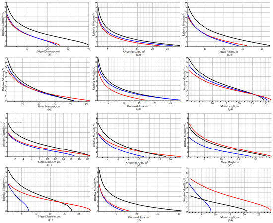
Figure 9.
Dynamics of relative mortality over mean diameter, mean occupied area, and mean height for mixed-effects scenario: (a1,a2,a3) all species of trees; (p1,p2,p3) pine species; (s1,s2,s3) spruce species; (b1,b2,b3) birch species; (p1,s1,b1) dynamic of relative mortality versus mean diameter; (p2,s2,b2) dynamic of relative mortality versus mean occupied area; and (p3,s3,b3) dynamic of relative mortality versus mean height.
Table 2 presents the potential for forecasting the number of trees per hectare using the newly developed mixed-effects parameters model. It utilizes fixed-effect parameter estimates from Table 1 and random effects for the occupied area calibrated using Equation (21) and the observed datasets. The presented model showed high goodness-of-fit statistical measures for the number of trees per hectare of live tree predictions in this region. For example, the root mean square error (percentage root mean square errors) for all species and pine, spruce, and birch species were 171.6 (15.4%), 130.1 (16.6%), 101.4 (24.2%), and 22.0 (30.0%), respectively, and the coefficient of determination for all species and pine, spruce, and birch species were 94.4%, 96.9%, 94.6%, and 95.8%, respectively.
Table 2.
Statistical measures * for the number of live trees per hectare model defined using Equation (22).
This paper suggests analyzing the instantaneous tree relative mortality in a forest stand using models based on stochastic differential equations. Higher predictability and interpretability are the primary benefits of newly developed stochastic differential equation models.
5. Conclusions
The main achievement of this study was the application of a 4-parameter Gompertz-type diffusion process to model tree mortality in mixed-species, uneven-aged stands. The normal copula function combined several diffusion processes and allowed the inclusion of not only age but also additional explanatory variables, such as tree diameter, height, crown base height, and crown width, to explain stand mortality. These newly derived probability density functions allow the formulation of equations describing the mean, quantile, and variance of the number of living and dead trees in mixed-species, uneven-aged forest stands.
Future work will focus on the derivation of multivariate distributions (e.g., diameter, height, and occupied area) with a general shape, which would allow the study of the basal area and volume and their increments of living and dead trees in a stand. To generate multivariate distributions, it is appropriate to use the copula method and stochastic differential equations.
Author Contributions
Conceptualization, E.P. and P.R.; Methodology, P.R.; Software, P.R.; Formal analysis, E.P. and P.R.; Data curation, E.P. and P.R.; Writing—original draft, P.R.; Writing—review & editing, E.P. and P.R.; Project administration, P.R. All authors have read and agreed to the published version of the manuscript.
Funding
This research was funded by the Horizon Europe Framework Programme (HORIZON) Teaming for Excellence (HORIZON-WIDERA-2022-ACCESS-01-two-stage), a creation of the Centre of Excellence in Smart Forestry “Forest 4.0”, No. 101059985. This research was co-funded by FOREST 4.0: “Ekscelencijos centras tvariai miško bioekonomikai vystyti” (No. 10-042-P-0002).
Data Availability Statement
Original data presented in this study are included in the main text, and field data presented in this study are available on request from the corresponding author.
Acknowledgments
The authors are very grateful to the Lithuanian Association of Impartial Timber Scalers for the sample dataset.
Conflicts of Interest
The authors declare no conflict of interest.
Appendix A
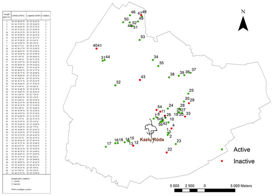
Figure A1.
The study area location.
References
- Del Río, M.; Oviedo, J.A.B.; Pretzsch, H.; Löf, M.; Ruiz-Peinado, R. A review of thinning effects on Scots pine stands: From growth and yield to new challenges under global change. For. Syst. 2017, 26, eR03S. [Google Scholar] [CrossRef]
- Hutchings, M.J.; Budd, C.S.J. Plant self-thinning and leaf area dynamics in experimental and natural monocultures. Oikos 1981, 36, 319–325. [Google Scholar] [CrossRef]
- Yoda, K. Self-thinning in overcrowded pure stands under cultivated and natural conditions (intraspecific competition among higher plants. J. Biol. Osaka City Univ. 1963, 14, 107–129. [Google Scholar]
- Lalor, A.R.; Law, D.J.; Breshears, D.D.; Falk, D.A.; Field, J.P.; Loehman, R.A.; Triepke, F.J.; Barron-Gafford, G.A. Mortality thresholds of juvenile trees to drought and heatwaves: Implications for forest regeneration across a landscape gradient. Front. For. Glob. Change 2023, 6, 1198156. [Google Scholar] [CrossRef]
- Morris, E. Self-thinning lines differ with fertility level. Ecol. Res. 2002, 17, 17–28. [Google Scholar] [CrossRef]
- Dhakal, T.; Cho, K.H.; Kim, S.-J.; Beon, M.-S. Modeling decline of mountain range forest using survival analysis. Front. For. Glob. Change 2023, 6, 1183509. [Google Scholar] [CrossRef]
- Rose, C.; Hall, D.; Shiver, B.; Clutter, M.; Borders, B. A Multilevel Approach to Individual Tree Survival Prediction. For. Sci. 2006, 52, 31–43. [Google Scholar] [CrossRef]
- Tian, X.; Sun, S.; Mola-Yudego, B.; Cao, T. Predicting individual-tree growth using stand-level simulation, diameter distribution and Bayesian calibration. Ann. For. Sci. 2020, 77, 57. [Google Scholar] [CrossRef]
- Fransson, P.; Brännström, A.; Franklin, O. A tree’s quest for light—Optimal height and diameter growth under a shading canopy. Tree Physiol. 2021, 41, 1–11. [Google Scholar] [CrossRef] [PubMed]
- Da Silva, B.G.; Demétrio, C.G.B.; Sermarini, R.A.; Molenberghs, G.; Verbeke, G.; Behling, A.; Marques, E.; Accioly, Y.; Figura, M.A. Height-Diameter Models: A Comprehensive Review with New Insights on Relationships to Generalized Linear Models and Differential Equations. Int. For. Rev. 2024, 26, 398–419. [Google Scholar] [CrossRef]
- Gärtner, A.; Jönsson, A.M.; Metcalfe, D.B.; Pugh, T.A.M.; Tagesson, T.; Ahlström, A. Temperature and Tree Size Explain the Mean Time to Fall of Dead Standing Trees across Large Scales. Forests 2023, 14, 1017. [Google Scholar] [CrossRef]
- Bradford, J.B.; Bell, D.M. A window of opportunity for climate-change adaptation: Easing tree mortality by reducing forest basal area. Front. Ecol. Environ. 2017, 15, 11–17. [Google Scholar] [CrossRef]
- Rogers, B.M.; Solvik, K.; Hogg, E.H.; Ju, J.; Masek, J.G.; Michaelian, M.; Berner, L.T.; Goetz, S.J. Detecting early warning signals of tree mortality in boreal North America using multiscale satellite data. Glob. Change Biol. 2018, 24, 2284–2304. [Google Scholar] [CrossRef]
- Rupšys, P. Understanding the Evolution of Tree Size Diversity within the Multivariate Nonsymmetrical Diffusion Process and Information Measures. Mathematics 2019, 7, 761. [Google Scholar] [CrossRef]
- Alzaatreh, A.; Aljarrah, M.; Almagambetova, A.; Zakiyeva, N. On the Regression Model for Generalized Normal Distributions. Entropy 2017, 23, 173. [Google Scholar] [CrossRef] [PubMed]
- Kohyama, T.S.; Potts, M.D.; Kohyama, T.I.; Kassim, A.R.; Ashton, P.S. Demographic properties shape tree size distribution in a Malaysian rain forest. Am. Nat. 2015, 185, 367–379. [Google Scholar] [CrossRef]
- Hara, T. A stochastic model and the moment dynamics of the growth and size distribution in plant populations. J. Theor. Biol. 1984, 109, 173–190. [Google Scholar] [CrossRef]
- Frank, S.A. An enhanced transcription factor repressilator that buffers stochasticity and entrains to an erratic external circadian signal. Front. Syst. Biol. 2023, 3, 1276734. [Google Scholar] [CrossRef]
- Maliyoni, M.; Gaff, H.D.; Govinder, K.S.; Chirove, F. Multipatch stochastic epidemic model for the dynamics of a tick-borne disease. Front. Appl. Math. Stat. 2023, 9, 1122410. [Google Scholar] [CrossRef]
- Mortoja, S.G.; Paul, A.; Panja, P.; Bhattacharya, S.; Mondal, S.K. Role Reversals in a Tri-Trophic Prey–Predator Interaction System: A Model-Based Study Using Deterministic and Stochastic Approaches. Math. Comput. Appl. 2024, 29, 3. [Google Scholar] [CrossRef]
- Leander, J.; Lundh, T.; Jirstrand, M. Stochastic differential equations as a tool to regularize the parameter estimation problem for continuous time dynamical systems given discrete time measurements. Math. Biosci. 2014, 251, 54–62. [Google Scholar] [CrossRef] [PubMed]
- Guo, W.; Ma, S.; Teng, L.; Liao, X.; Pei, N.; Chen, X. Stochastic differential equation modeling of time-series mining induced ground subsidence. Front. Earth Sci. 2023, 10, 1026895. [Google Scholar] [CrossRef]
- Ito, K. On Stochastic Differential Equations. Mem. Amer. Math. Soc. 1951, 4, 1–51. [Google Scholar] [CrossRef]
- Krikštolaitis, R.; Mozgeris, G.; Petrauskas, E.; Rupšys, P. A Statistical Dependence Framework Based on a Multivariate Normal Copula Function and Stochastic Differential Equations for Multivariate Data in Forestry. Axioms 2023, 12, 457. [Google Scholar] [CrossRef]
- Ditlevsen, S.; Samson, A. Introduction to Stochastic Models in Biology. In Stochastic Biomathematical Models; Lecture Notes in Mathematics; Springer: Berlin/Heidelberg, Germany, 2013; Volume 2058. [Google Scholar]
- Pouta, P.; Kulha, N.; Kuuluvainen, T.; Aakala, T. Partitioning of Space Among Trees in an Old-Growth Spruce Forest in Subarctic Fennoscandia. Front. For. Glob. Change 2022, 5, 817248. [Google Scholar] [CrossRef]
- Rupšys, P.; Narmontas, M.; Petrauskas, E. A Multivariate Hybrid Stochastic Differential Equation Model for Whole-Stand Dynamics. Mathematics 2020, 8, 2230. [Google Scholar] [CrossRef]
- Seo, Y.; Lee, D.; Choi, J. Developing and Comparing Individual Tree Growth Models of Major Coniferous Species in South Korea Based on Stem Analysis Data. Forests 2023, 14, 115. [Google Scholar] [CrossRef]
- Güner, Ş.T.; Diamantopoulou, M.J.; Özçelik, R. Diameter distributions in Pinus sylvestris L. stands: Evaluating modelling approaches including a machine learning technique. J. Forestry Res. 2023, 34, 1829–1842. [Google Scholar] [CrossRef]
- Räty, J.; Hietala, A.M.; Breidenbach, J.; Astrup, R. An analysis of stand-level size distributions of decay-affected Norway spruce trees based on harvester data. Ann. For. Sci. 2023, 80, 2. [Google Scholar] [CrossRef]
- Fu, Y.; He, H.S.; Wang, S.; Wang, L. Combining Weibull distribution and k-nearest neighbor imputation method to predict wall-to-wall tree lists for the entire forest region of Northeast China. Ann. For. Sci. 2022, 79, 42. [Google Scholar] [CrossRef]
- Sa, Q.; Jin, X.; Pukkala, T.; Li, F. Developing Weibull-based diameter distributions for the major coniferous species in Hei-longjiang Province, China. J. Forestry Res. 2023, 34, 1803–1815. [Google Scholar] [CrossRef]
- Øksendal, B.K. An Introduction with Applications. In Stochastic Differential Equations; Springer: Berlin/Heidelberg, Germany, 2023. [Google Scholar]
- Sklar, M. Fonctions de repartition an dimensions et leurs marges. Publ. Inst. Statist. Univ. Paris 1959, 8, 229–231. [Google Scholar]
- Rupšys, P.; Mozgeris, G.; Petrauskas, E.; Krikštolaitis, R. A Framework for Analyzing Individual-Tree and Whole-Stand Growth by Fusing Multilevel Data: Stochastic Differential Equation and Copula Network. Forests 2023, 14, 2037. [Google Scholar] [CrossRef]
- Ciceu, A.; Chakraborty, D.; Ledermann, T. Examining the transferability of height–diameter model calibration strategies across studies. Forestry 2023, 2023, cpad063. [Google Scholar] [CrossRef]
- Rupšys, P.; Petrauskas, E. On the Construction of Growth Models via Symmetric Copulas and Stochastic Differential Equations. Symmetry 2022, 14, 2127. [Google Scholar] [CrossRef]
- Efron, B.; Hinkley, D.V. Assessing the accuracy of the maximum likelihood estimator: Observed versus expected Fisher In-formation. Biometrika 1978, 65, 457–487. [Google Scholar] [CrossRef]
- Reineke, L.H. Perfecting a stand-density index for even-aged forests. J. Agric. Res. 1933, 46, 627–630. [Google Scholar]
- Neumann, M.; Adams, M.A.; Lewis, T. Native Forests Show Resilience to Selective Timber Harvesting in Southeast Queens-land, Australia. Front. For. Glob. Change 2021, 4, 750350. [Google Scholar] [CrossRef]
- Tian, D.; Bi, H.; Jin, X.; Li, F. Stochastic frontiers or regression quantiles for estimating the self-thinning surface in higher di-mensions? J. Forestry Res. 2021, 32, 1515–1533. [Google Scholar] [CrossRef]
- Mrad, A.; Manzoni, S.; Oren, R.; Vico, G.; Lindh, M.; Katul, G. Recovering the Metabolic, Self-Thinning, and Constant Final Yield Rules in Mono-Specific Stands. Front. For. Glob. Change 2020, 3, 62. [Google Scholar] [CrossRef]
- McCune, B.; Cottam, G. The successional status of a southern Wisconsin oak woods. Ecology 1985, 66, 1270–1278. [Google Scholar] [CrossRef]
- Sheil, D.; May, R.M. Mortality and recruitment rate evaluations in heterogeneous tropical forests. J. Ecol. 1996, 84, 91–100. [Google Scholar] [CrossRef]
- Westoby, M. The Self-Thinning Rule. Adv. Ecol. Res. 1984, 14, 167–225. [Google Scholar]
- Pavel, M.A.A.; Barreiro, S.; Tomé, M. The Importance of Using Permanent Plots Data to Fit the Self-Thinning Line: An Example for Maritime Pine Stands in Portugal. Forests 2023, 14, 1354. [Google Scholar] [CrossRef]
- Gavrikov, V.L. A simple theory to link bole surface area, stem density and average tree dimensions in a forest stand. Eur. J. For. Res. 2014, 133, 1087–1109. [Google Scholar] [CrossRef]
Disclaimer/Publisher’s Note: The statements, opinions and data contained in all publications are solely those of the individual author(s) and contributor(s) and not of MDPI and/or the editor(s). MDPI and/or the editor(s) disclaim responsibility for any injury to people or property resulting from any ideas, methods, instructions or products referred to in the content. |
© 2025 by the authors. Licensee MDPI, Basel, Switzerland. This article is an open access article distributed under the terms and conditions of the Creative Commons Attribution (CC BY) license (https://creativecommons.org/licenses/by/4.0/).