Data-Driven Two-Stage Distributionally Robust Mean Semi-Variance Mixed-Integer Optimization Model for Location Allocation Problems in an Uncertain Environment

Abstract

This study considers the uncertainty caused by data asymmetry in supply chains, the risks associated with this uncertainty and the need for robustness in the supply chain network. It discusses the construction of a data-driven two-stage distributionally robust mean semi-variance mixed-integer optimization model to address the location optimization problem under conditions of uncertainty in transportation costs and demand. To solve this model, a distributed separation hybrid genetic algorithm is introduced, enabling determination of the optimal location, distribution strategy and expected return for a distribution center in the worst case. Then, a fresh food supply chain is utilized as a case study to analyze the effects of uncertainty on location allocation decisions while deriving pertinent managerial insights. Additionally, compared to traditional stochastic optimization models, the proposed model demonstrates greater robustness in numerical simulations. The algorithm is also benchmarked against other methods, and its effectiveness and stability are validated in terms of the computational time, the number of iterations and the convergence speed.

1. Introduction

With continuous improvements in income and consumption levels, people’s demand for high-quality, personalized and experiential consumption is growing, which prompts enterprises to focus on improving the customer experience and continuously improving the service level from the perspective of customers, centering on logistics and transportation. By strengthening the construction of logistics informatization, enterprises can accurately predict the quantity of products sold, allocate products and provide services to customers with higher efficiency, lower cost and a better service experience. Nowadays, many enterprises are starting to manage the quantity of products shipped through the new approach of “Internet + logistics”. The basic approach is to analyze the historical data for enterprise products, coordinate the relationship between goods and transportation and realize seamless connections between logistics nodes [1,2]. At this time, the location of logistics nodes and the transportation scheme are among the most pivotal and strategic considerations in the planning and operation of supply chain networks. How to use historical data information to optimize the location allocation in supply chain networks is a problem worthy of further study.

Supply chain management involves numerous uncertainties. For instance, demand forecasting is subject to unpredictability due to factors such as fluctuating economic conditions, shifts in consumer psychology and a lack of historical demand data. This also leads to information asymmetry in transportation costs among suppliers, distribution centers and customers, further contributing to uncertainty. A reliable supply chain system is particularly crucial for meeting the volatile demands of customers. Although most supply chains are relatively sound and usually operate effectively, when events such as global health crises occur, various weaknesses are often exposed in supply chains, and they cannot provide real flexibility. For example, the outbreak of COVID-19 undoubtedly brought greater uncertainty to the global supply chain, which means the supply chain system needs robustness, and a distributionally robust optimization method can solve this problem [3,4,5]. Therefore, this study examines the location allocation problem by using a distributionally robust optimization method which makes the supply chain system more robust. In contrast to stochastic programming, which typically presumes that the probability distribution of random parameters is known beforehand, the core concept of the distributed robust optimization approach is the building of an uncertainty set that encompasses the true probability distribution, centered around a reference distribution [6,7].

In recent years, a two-stage stochastic optimization model has become a research hotspot within modern optimization methods. It divides the whole decision-making process into two stages. The first stage is the “here and now” decision, which must be carried out before the value of the random vector is realized. The second stage is the “wait and see” decision, which can be used as retrospective behavior for the first-stage decision after the value of the random vector is realized. The two-stage stochastic optimization model has been extensively applied across various domains, including financial portfolio management, supply chain operations, emergency resource allocation and smart grid systems [8,9,10,11,12,13].

Furthermore, the majority of location problems adopt a risk-neutral approach, which means that they focus on optimizing the expected cost (or the expected profit) as the objective function without accounting for risk [4,14,15,16,17,18]. In contrast, risk-averse methods take into account the variability in random outcomes, offering a more robust framework for decision-making under uncertainty. This allows decision-makers to assess strategies based on their individual risk preferences. Given the challenges posed by actual market fluctuations, this paper incorporates risk considerations to derive more effective and practical solutions. The variance risk measure is a commonly used risk measure which regards both positive and negative fluctuations that deviate from the expected return as risks. The lower-half variance measure only regards the negative deviation below the expected return as risk. It can be seen that the use of a semi-variance measurement is more in line with people’s perception of risk than a variance risk measurement. As far as we know, no previous studies have used a two-stage distributionally robust mean semi-variance mixed-integer optimization model to study location allocation in the supply chain. Therefore, this paper uses the semi-variance risk measure as the risk measure for this purpose. Based on the above discussion, this study examines how to build a data-driven two-stage distributionally robust mean semi-variance mixed-integer optimization model to discuss the location optimization problem under uncertainty in the transportation cost and demand.

There are two common algorithms for two-stage distributed robust optimization: a decomposition algorithm [12,19] and a distribution separation algorithm [20,21]. In this paper, because the first-stage decision variables are integers and semi-variance risk applies, it is difficult to apply transformation for dual problems. Thus, this paper utilizes the concept of distributional separation to solve a distributionally robust optimization problem. Additionally, Medsker [22] introduced several innovative methodologies for developing hybrid intelligent algorithms, providing a foundational framework for addressing mixed-integer programming problems. As far as we know, there is still a lack of research on the application of intelligent algorithms to solve the two-stage distribution robust mean semi-variance optimization problem. A genetic algorithm is an adaptive global optimization search algorithm that simulates the genetic and evolutionary processes of organisms in the natural environment. A genetic algorithm is an efficient, practical and robust optimization technology which can effectively solve NP problems. Therefore, drawing on the principles of distributed separation and genetic algorithms, this study presents a novel solution framework known as the distributed separation hybrid genetic algorithm. The primary contributions of this research are outlined below.

⋆

In light of the uncertainty arising from data asymmetry within the supply chain, a two-stage distributionally robust mean semi-variance mixed-integer optimization model is developed.

⋆

A distributed separation hybrid genetic algorithm for solving the two-stage distributionally robust mean semi-variance mixed-integer optimization model is proposed. The effectiveness of the algorithm is verified by comparison.

⋆

In an example, management opinions are put forward.

The rest of this paper is organized as follows: Section 2 is a literature review. Section 3 includes the preliminary knowledge, and introduces the concepts related to risk measurement and time uncertainty. Section 4 establishes the model. In Section 5, a distributed separation hybrid genetic algorithm is proposed. Section 6 verifies the effectiveness of the model and algorithm through an example. Section 7 is the conclusion.

2. Literature Review

Location allocation problems are widely applied in industrial, civil and defense sectors, such as in the siting of logistics centers, warehouses and military bases. They directly impact operational efficiency and service quality, making them a long-standing focus of academic and industrial research and a key interdisciplinary topic. Hu et al. [4] investigated the multi-period hub location problem with uncertain periodic demand. Nick et al. [23] developed a location–inventory allocation model for post-disaster humanitarian logistics distribution points, emphasizing both the temporal dynamics of the system and potential social cost factors in facility location decisions. Qi et al. [24] investigated the competitive facility location problem, formulating a bilevel mixed-integer nonlinear programming model and developing a solution algorithm with guaranteed constant-factor approximation performance. Liu et al. [25,26] studied the location problem of distribution centers in supply chain networks with random transportation costs and demand. To address supply chain risk uncertainty, they established a mean-risk optimization model and developed heuristic algorithms to solve it.

In most studies on location allocation problems, uncertainty is typically based on randomness, with the assumption that the probability information of uncertainty is known [14,15,16,17,18,27]. However, in many cases, historical data or reliable forecasting techniques to derive accurate probability information are limited. Soyster [28] introduced a robust optimization approach to tackle challenges related to data uncertainty and the unavailability of probabilistic information.

In recent years, two-stage stochastic programming has emerged as a pivotal branch of modern optimization theory, garnering significant academic attention. This methodology has demonstrated remarkable value across multiple practical applications, including financial asset allocation, supply chain optimization scheduling, emergency resource distribution and smart energy networks. Atamturk et al. [8] introduced a two-stage robust optimization method to address the network flow design problem under conditions of demand uncertainty. Nakao et al. [9] studied stochastic network design problems through a two-stage approach. In the first stage, network capacity is designed, while, in the second stage, single-commodity network traffic is optimized after demand realization. The model aims to minimize total costs, including network capacity allocation, goods flow and penalties for unmet demand. Zhang et al. [10] constructed a multi-microgrids cooperative operation model based on two-stage adaptive robust optimization, and discussed how to minimize the operating cost of the microgrid combination in the worst case when PV was uncertain. Zhang et al. [11] constructed a two-stage distributionally robust optimization model and studied the storage and scheduling problems of a natural gas–electric hybrid energy system under uncertain wind power. Lei et al. [12] proposed a two-stage robust optimization model for the size and routing of mobile device clusters under uncertain demand, and gave a solution method based on the bilevel cut plane. Ding et al. [13] employed a two-stage robust optimization framework to investigate the reactive power optimization problem associated with uncertain wind power integration in active distribution networks. Ling et al. [29] proposed a two-stage distributionally robust optimization model based on moment constraints with risk aversion, equivalently transformed the model into semidefinite programming for solution and applied the constructed model to study supply chain management and portfolio problems.

Addressing the two-stage stochastic optimization model generally presents greater complexity, as it involves computing the expected value of multivariate random variables. A widely used approach for solving such problems is the scenario-based stochastic optimization method [30,31]. However, the effectiveness of this method heavily depends on the predefined scenarios and their associated probabilities. Moreover, as the number of scenarios increases, the computational complexity grows exponentially, leading to the curse of dimensionality.

Moreover, most location problems adopt a risk-neutral approach. For example, Laporte et al. [14] addressed the capacitated facility location problem with stochastic demands and developed a novel modeling approach based on two-stage stochastic integer programming. Wang et al. [15] explored facility location optimization under demand uncertainty with fixed server constraints. Zadeh et al. [16] investigated the strategic and tactical design of iron and steel supply chain networks. Armas et al. [17] studied the uncapacitated facility location problem with stochastic demands and proposed a simheuristic algorithm for solving it. Li et al. [18] optimized equipment support depot location and transportation allocation under multiple constraints using an uncertain chance-constrained programming approach. To overcome the limitations of traditional risk-neutral optimization methods (which focus solely on expected costs/profits while neglecting risk factors), this study proposes a risk-averse approach that better aligns with real-world decision-making needs. Specifically, it employs a semi-variance risk measure (considering only negative deviations) instead of the traditional variance measure (accounting for both positive and negative deviations) to better reflect human risk perception. A novel two-stage distributionally robust mean semi-variance mixed-integer optimization model for supply chain location allocation problems is developed, providing robust solutions for volatile market environments.

Based on the aforementioned analysis, this study proposes a data-driven two-stage distributionally robust optimization approach to address location problems under uncertainties in both transportation costs and demand, integrating mean semi-variance risk measures with mixed-integer programming techniques. When solving two-stage distributionally robust optimization problems, two predominant algorithmic approaches are typically employed: decomposition algorithms [12,14,19] and distribution separation algorithms [20,21,26]. This study proposes an innovative distribution separation technique to construct a solution framework, overcoming the duality transformation challenges caused by integer-constrained first-stage decision variables and semi-variance risk measures.

3. Preliminaries

Risk measures are mathematical functions that quantify risks associated with random variables through scalar values, offering a method to evaluate and compare outcomes according to decision-makers’ risk preferences. The variance risk measure considers both positive and negative fluctuations deviating from expected returns as risks. The semi-variance risk measure treats only negative deviations below expected returns as risks, or positive deviations above expected costs as risks. It can be seen that using the semi-variance risk measure is more consistent with people’s cognition of risk than the variance risk measure. Next, we give the definition of semi-variance:

Definition 1.

Let ξ be a random cost variable. If $E{\left[{(\xi -E\left[\xi \right])}^{+}\right]}^2$ exists, $E{\left[{(\xi -E\left[\xi \right])}^{+}\right]}^2$ is called the semi-variance of ξ, denoted as $SVaR\left(\xi \right)$, that is,

$$SVaR\left(\xi \right)=E{\left[{(\xi -E\left[\xi \right])}^{+}\right]}^2,$$

where ${\left(x\right)}^{+}=max(0,x).$

To facilitate the solution, we give some properties of SVaR:

Proposition 1.

If ξ is a random cost variable and C is a constant, then

$$SVaR(C+\xi )=SVaR\left(\xi \right).$$

Proof. 

By definition, we obtain

$$\begin{array}{ccc}\hfill \mathrm{SVaR}(C+\xi )& & =E{\left[{(C+\xi -E[C+\xi ])}^{+}\right]}^2\hfill \\ \hfill & & =E{\left[{(\xi -E\left[\xi \right])}^{+}\right]}^2\hfill \\ \hfill & & =\mathrm{SVaR}\left(\xi \right).\hfill \end{array}$$

  □

The objective of uncertainty quantification is to certify that a given physical, engineering or economic system satisfies multiple safety conditions with high probability. In this paper, we assume that the system parameters are governed by an ambiguous distribution, which is only known to belong to a prescribed ambiguity set.

Definition 2.

Let the random vector ξ be defined in the probability space $(\Omega ,\mathcal{F},\mathcal{P})$, where $\Omega ={\mathbb{R}}^n$. It is assumed that the first moment (mean) and the second moment (covariance) of the random vector $\xi \in \Omega$ are known. Denote $\mu =E_P\left[\xi \right]\in {\mathbb{R}}^n$ as the expected value (mean vector) and $\sum =E_P\left[(\xi -\mu ){(\xi -\mu )}^T\right]\in {\mathbb{S}}^n$ as the covariance matrix of ξ. The ambiguity set, comprising all random vectors that share the same first and second moments, is formally defined as follows:

$$\mathcal{P}:=\{P:{\int }_{\xi \in \Omega }P\left(\xi \right)d\xi =1,{\int }_{\xi \in \Omega }\xi P\left(\xi \right)d\xi =\mu ,{\int }_{\xi \in \Omega }\xi {\xi }^{T}P\left(\xi \right)d\xi =\Sigma +\mu {\mu }^T\}.$$

4. Problem Description and Two-Stage Distributionally Robust Mean Semi-Variance Mixed-Integer Optimization Model

With the increasing demand for fresh products, the construction of fresh product supply chains is gradually accelerating. Although the traditional fresh supply chain can promote the circulation of products in the market, the turnover times and circulation time are long, it is easy to cause serious damage to fresh products and sales prices are high.

Since the application of Internet technology in the construction of fresh product supply chains, these problems have been effectively alleviated. With the operation mode of e-commerce platform supply chains, consumers can have organic interaction with producers and promote the fresh product market from being product led to being service led. After several years of exploration and development, a fresh food chain enterprise has established a three-tier structure of online sales supply chain model, that is, “supplier—distribution center—consumer”, from the production, procurement, storage and distribution of goods in the whole process. Through the app, enterprises can collect customers’ shopping information, analyze their demand preferences and then predict the market demand trend, make procurement plans and meet consumers’ demands for diversified products. After the fresh products are purchased from the planting base or locally, the quality of the fresh products is tested, the products are stored and packaged at low temperatures and the raw materials or semi-finished products are reprocessed and transported to the distribution center.

The aim of this paper is to solve the problem that, in the worst case, considers the choice of distribution center and fresh distribution to ensure that customers receive orders in the shortest time. It is assumed that the distribution of only one kind of goods is considered in the location allocation problem. In the context of uncertain demand and transportation costs, the decision of the first stage is to choose the distribution center. In the second stage, after determining the selected distribution center, the distribution scheme is decided. The goal is to minimize total costs within the constraints of meeting requirements. In order to introduce the application of the two-stage distributionally robust mean semi-variance mixed-integer optimization model into fresh location distribution, relevant parameters and symbols are shown below.

For the sake of simplicity, the following notation is adopted throughout this model. All vectors referenced in this study are assumed to be column vectors by default.    

Symbol	Definition
Notation
I	The set of suppliers.
J	The set of distribution centers.
K	The set of customers.
Parameters
$a_i$	The ability of supplier i to supply products, $i\in I$.
$C{p}_i$	The product cost, $i\in I$.
$C{u}_i$	The cost of processing a unit of product by supplier i, $i\in I$.
$C{d}_j$	Fixed cost of operating distribution center j, $j\in J$.
$e_j$	Distribution capacity of distribution center j, $j\in J$.
r	Retail price of a unit product.
${\tilde{m}}_{ij}$	Transportation cost from supplier i to distribution center j (random variable).
${\tilde{n}}_{jk}$	Distribution cost from center j to customer k (random variable).
${\tilde{w}}_k$	Demand of customer k (random variable).
$\xi \left(\omega \right)$	Demand and transportation cost vector $\xi \left(\omega \right)=({\tilde{m}}_{ij}\left(\omega \right),{\tilde{n}}_{jk}\left(\omega \right),$ ${\tilde{w}}_k\left(\omega \right))$, $\omega \in \Omega$ (random variable).
$\lambda$	Weight of cost.
$E(·)$	Expectation.
Decision variables
${\beta }_j$	0–1 decision variable: 1 means open distribution center j; otherwise 0, $j\in J$.
$x_{ij}$	Quantity of products transported from supplier i to distribution center j, $i\in I$, $j\in J$.
$y_{jk}$	Quantity of products transported from distribution center j to customer k, $j\in J$, $k\in K$.

Assume that random variables are independent of each other. Based on the above description, we establish a data-driven two-stage distributionally robust mean semi-variance mixed-integer optimization model. The model considers the expected cost of the supply chain and its risk minimization, and is obtained by the convex combination of the risk measure function and the expected cost function, that is, the convex combination is used to transform multi-objective programming into single-objective programming. As a function of the random parameter vector $\xi \left(\omega \right)$, the total cost ${\sum }_{J}C{d}_j{\beta }_j+Q(\beta ,\xi \left(\omega \right))$ is obviously a random variable. What is higher than the expected cost is regarded as the risk (that is, the part lower than the expected benefit), and the risk function can be expressed as $\mathrm{SVaR}({\sum }_{J}C{d}_j{\beta }_j+Q(\beta ,\xi \left(\omega \right)))$. It follows from the property of semi-variance that $\mathrm{SVaR}({\sum }_{J}C{d}_j{\beta }_j+Q(\beta ,\xi \left(\omega \right)))$ = $\mathrm{SVaR}\left(Q\right(\beta ,\xi \left(\omega \right)\left)\right)$. We focus on optimizing the expected cost and minimizing risk within the supply chain under the worst-case scenario. That is, ${min}_{\beta }{sup}_{p\in \mathcal{P}}\{\lambda ({\sum }_{J}C{d}_j{\beta }_j+E_p\left[Q(\beta ,\omega )\right])+(1-\lambda )\mathrm{SVaR}({\sum }_{J}C{d}_j{\beta }_j+Q(\beta ,\xi \left(\omega \right)))\}$.

Next, we present a data-driven two-stage distributionally robust mean semi-variance mixed-integer optimization model as follows:

$$\begin{array}{c}\underset{\beta }{min}\lambda \sum _{J}C{d}_j{\beta }_j+\underset{p\in \mathcal{P}}{sup}\{\lambda E_p\left[Q(\beta ,\xi \left(\omega \right))\right]+(1-\lambda )\mathrm{SVaR}\left(Q(\beta ,\xi \left(\omega \right))\right)\}\hfill \\ \mathrm{s}.\mathrm{t}.\beta \in {\{0,1\}}^J.\hfill \end{array}$$

(1)

where $\mathcal{P}$ represents the uncertain set containing the real distribution, and $Q(\beta ,\omega )$ is the optimal value for the following second-stage problem:

$$\begin{array}{c}Q(\beta ,\xi \left(\omega \right))=\underset{\mathbf{x},\mathbf{y}}{\min }\{\sum _I\sum _{J}C{p}_i{x}_{ij}+\sum _I\sum _{J}C{u}_i{x}_{ij}+\sum _I\sum _J{\tilde{m}}_{ij}{x}_{ij}\hfill \\ +\sum _J\sum _K{\tilde{n}}_{jk}{y}_{jk}-\sum _J\sum _{K}r{y}_{jk}\}\hfill \end{array}$$

(2)

$$\begin{array}{cc}\hfill \mathrm{s}.\mathrm{t}.& \sum _J{x}_{ij}\le a_i\forall i\in I,\hfill \end{array}$$

(2a)

$$\begin{array}{c}\sum _K{y}_{jk}\le {\beta }_j{e}_j\forall j\in J,\hfill \end{array}$$

(2b)

$$\begin{array}{c}\sum _K{y}_{jk}\le \sum _I{x}_{ij}\forall j\in J,\hfill \end{array}$$

(2c)

$$\begin{array}{c}\sum _J{y}_{jk}={\tilde{w}}_k\left(\omega \right)\forall k\in K,\hfill \end{array}$$

(2d)

$$\begin{array}{c}{x}_{ij},y_{jk}\ge 0,\forall i\in I,j\in J,k\in K.\hfill \end{array}$$

(2e)

This representation clearly indicates the order of events. The first-stage decision variable $\beta$ is solved in the case of uncertainties in $\omega$, and the effects of these uncertainties are measured by the backtracking function $E_p\left[Q(\beta ,\xi \left(\omega \right))\right]$. In the second stage, the actual value of $\omega$ is given and the traceability decision $\mathbf{x},\mathbf{y}$ is solved.

In the model, the objective function (1) aims to minimize both the expected cost and the associated risk of the supply chain in the worst case. The second stage minimizes the cost function (2), which includes product cost, handling cost, transportation cost and revenue from selling the product. Constraints (2a) and (2b) represent the supply capacity constraints of suppliers and the distribution capacity constraints of distribution centers, respectively. Constraint (2c) represents the equilibrium condition of the product. Constraint (2d) means to meet the needs of consumers. The final constraint (2e) guarantees the non-negativity of the decision variable.

5. Solution Algorithm

This section discusses the algorithm for solving models (1) and (2). Without loss of generality, in the subsequent analysis, we denote ${\xi }_s\left(\omega \right)$ as the random variable in scenario s, with $p_s$ (unknown) representing its corresponding probability, $s\in S$ and S as the set of all possible scenarios.

In the two-stage distributionally robust mean semi-variance mixed-integer optimization models (1) and (2), when $\lambda =1$, Equation (1) degenerates into a two-stage risk-neutral distributionally robust optimization model, and some scholars have studied its robust equivalent transformation. Thereafter, the robust equivalent equation is solved [6]. When $\lambda \ne 1$, because the risk function SVaR is a nonlinear function and there are integer constraints in the decision variables, the problem in the first stage is a nonlinear distributionally robust mixed-integer optimization problem. All this makes it more complicated to obtain a robust equivalent of the original problem. In addition, notice that, for each $\xi \left(\omega \right)$, the second-stage problem has $2\left|I\right|+3\left|J\right|+2\left|K\right|$ constraints, which makes it very difficult to solve the two-stage distributionally robust mean semi-variance mixed-integer optimization model when scenario $\left|S\right|$ is very large or the supply chain has a large number of members.

It is important to note that the two-stage distributionally robust mixed-integer optimization model is at least as complex as the two-stage random mixed-integer optimization model, which represents a specific instance of the former. Given that the two-stage random mixed-integer optimization problem is NP hard, this implies a significant computational challenge. To address such problems, several researchers have employed the idea of distribution separation within the framework of robust optimization [20,26]. This idea directly avoids the transformation of robust equivalence and solving large-scale robust equivalence (when there are many scenarios or many supply chain members). In addition, the idea of a hybrid intelligent algorithm lays a foundation for solving mixed-integer optimization problems [32]. A GA is an adaptive global optimization search technique inspired by the genetic and evolutionary mechanisms observed in biological organisms within natural environments. A GA is an efficient, practical and robust optimization technology which can solve NP problems effectively. Therefore, leveraging the principles of distribution separation and genetic algorithms, this study proposes a solution framework termed the distribution separation hybrid genetic algorithm, with the detailed solution procedure illustrated in Figure 1. First, the first-stage problem is solved, where the decision vector $\beta$ is the first-stage decision that must be determined before the random transportation costs and demand vector $\xi \left(\omega \right)$ are realized. Then, in the second-stage, given the realized random transportation costs, demand $\xi \left(\omega \right)$ and the first-stage decision $\beta$, the second-stage problem is solved to obtain the optimal solution $\mathbf{x},\mathbf{y}$ and the optimal value $Q(\beta ,\xi (\omega \left)\right)$. By solving the distribution separation problem, the optimal probability distribution p is derived. The process then returns to the first stage, repeating the above cycle until the obtained optimal solution stabilizes.

The optimization problem

$$\begin{array}{c}\mathcal{Q}:=\underset{p\in \mathcal{P}}{sup}\{\lambda E_p\left[Q(\beta ,\xi \left(\omega \right))\right]+(1-\lambda )\mathrm{SVaR}\left(Q(\beta ,\xi \left(\omega \right))\right)\}\hfill \end{array}$$

(3)

is called the distribution separation problem. The algorithm for solving (3) is called the distribution separation algorithm [20].

Next, we describe the solution process in detail.

$X=({\beta }_1,{\beta }_2,\cdots ,{\beta }_J)$, where the population consists of N individuals. Initial population $B=\{B_1,B_2,\cdots ,B_N\}$. $Fit(·)$ is a fitness function, and the fitness of each individual is the negative of the value of the function in the first stage, that is,

$$\begin{array}{c}\hfill Fi{t}_n\left(X\right)=-\{\lambda \sum _{J}C{d}_j{\beta }_j+\underset{p\in \mathcal{P}}{sup}\{\lambda E_p\left[Q(\beta ,\xi \left(\omega \right))\right]+(1-\lambda )\mathrm{SVaR}\left(Q(\beta ,\xi \left(\omega \right))\right)\}\},n\in N.\end{array}$$

(4)

Therefore, the smaller the function value in the first stage, the higher the fitness value. For each $\xi \left(\omega \right)$, the interior point algorithm is used to solve the problem of the second stage (2).

If the selection strategy adopts roulette wheel selection, it is necessary to rotate the wheel N times when selecting N individuals, and the calculation is complicated. In order to improve this problem, this paper adopts stochastic universal sampling. If N individuals are selected, N individuals can be selected by generating N equally spaced marker pointer positions once. Assuming that the total fitness value is $F=\sum \left(Fi{t}_n\left(X\right)\right)$ and the number of individuals is N, the specific steps of stochastic universal sampling are as follows:

step1: 

Calculate the pointer spacing $P=F/N$;

step2: 

Randomly generate the starting point pointer position Start = [random number between 0 and P];

step3: 

Calculation of the position of the pointer Pointers =  [Start $+i\ast P(i=(0,1,\dots ,N-1\left)\right)$];

step4: 

Select N individuals according to the position of each pointer. Select and replicate, and the duplicated chromosomes form population $B1$.

Next, a crossover operation is performed. This paper adopts a crossover operation based on probability. According to the number of chromosomes $\overline{c}$ participating in the crossover, determined by crossover rate $Pc$, $\overline{c}$ chromosomes are randomly selected from $B1$ which are paired for the crossover operation, and the resulting new chromosomes are used to replace the original chromosomes to obtain population $B2$.

According to the variation times m determined by the variation rate $Pm$, m chromosomes are randomly determined from $B2$, and the variation operations are carried out, respectively, and the new chromosomes are used to replace the original chromosomes to obtain population $B3$. Population $B3$ is taken as the new generation population, that is, $B3$ replaces B. The fitness $Fit\left(X\right)$ of each chromosome in B is calculated again until the termination condition is met. Next, we present the pseudo-code of Algorithm 1.

Algorithm 1 Distribution separation hybrid genetic algorithm (DSHGA).

Initialization. The population size is N, maximum number of iterations G, crossover rate $Pc$, mutation rate $Pm$, randomly obtain the initial population $B=randint(N,J)$; Genetic algorithms iterate. for g = 1:G do     Calculate the fitness     for n = 1:N do         The second stage optimization problem (2) is addressed utilizing the interior point algorithm;         The distribution separation problem (3) is solved to obtain the value of $\mathcal{Q}$;         Calculate the fitness $Fi{t}_n\left(X\right)$ for each chromosome in B;     end for     Obtain the optimal individual $X_{Best}$;     Stochastic universal sampling     Calculate the pointer spacing $P=\sum \left(Fi{t}_n\left(X\right)\right)/N$;     Randomly generate the starting point pointer position Start = [random number between 0 and P];     Calculation of the position of the pointer Pointers = [Start $+i\ast P(i=0,1,\dots ,N-1)$];     Select N individuals according to the position of each pointer.     Crossover operation     for n = 1:2:N do         if $rand<Pc$ then            crossover chromatid;         end if     end for     Get population $B2$;     Mutation operation     for n = 1:N do         for j = 1:J do            if $rand<Pm$ then                Mutation;            end if         end for     end for     Get population $B3$;     The optimal individual $X_{Best}$ is kept in the new species group $B3$; end for Return the ${\mathbf{X}}_{best}$ as the optimal solution, and $-Fit\left({\mathbf{X}}_{best}\right)$ as the optimal value.

6. Numerical Results

In this section, the impact of uncertainty on the location of distribution centers is examined using the fresh supply chain in Shanghai as a case study. All the program codes were written on MATLAB R2014a using Lenovo computers running an Intel(R) Core(TM) i7-8565U CPU @ 1.80 GHz, 8.00 GB memory. In the whole calculation experiment, the parameters of the DSHGA are set as $G=1000$, $N=500$, $Pc=0.9$, $Pm=0.05$, $\lambda =0.9.$

In the numerical table, $Pro=-\{{\sum }_{J}C{d}_j{\beta }_j+{sup}_{p\in \mathcal{P}}\left\{E_p\left[Q(\beta ,\xi \left(\omega \right))\right]\right\}\}$ represents the profit of the supply chain in the worst case, $Val$ represents the optimal value of model (1) and ${\beta }^{*}$ is the optimal solution. $x_{ij}^{*}$ represents the quantity of product shipped from supplier i to distribution center j. $y_{jk}^{*}$ represents the quantity of product shipped from distribution center j to demand area k. $TI$ indicates the computation time, in seconds. Next, we give a description of the test problem.

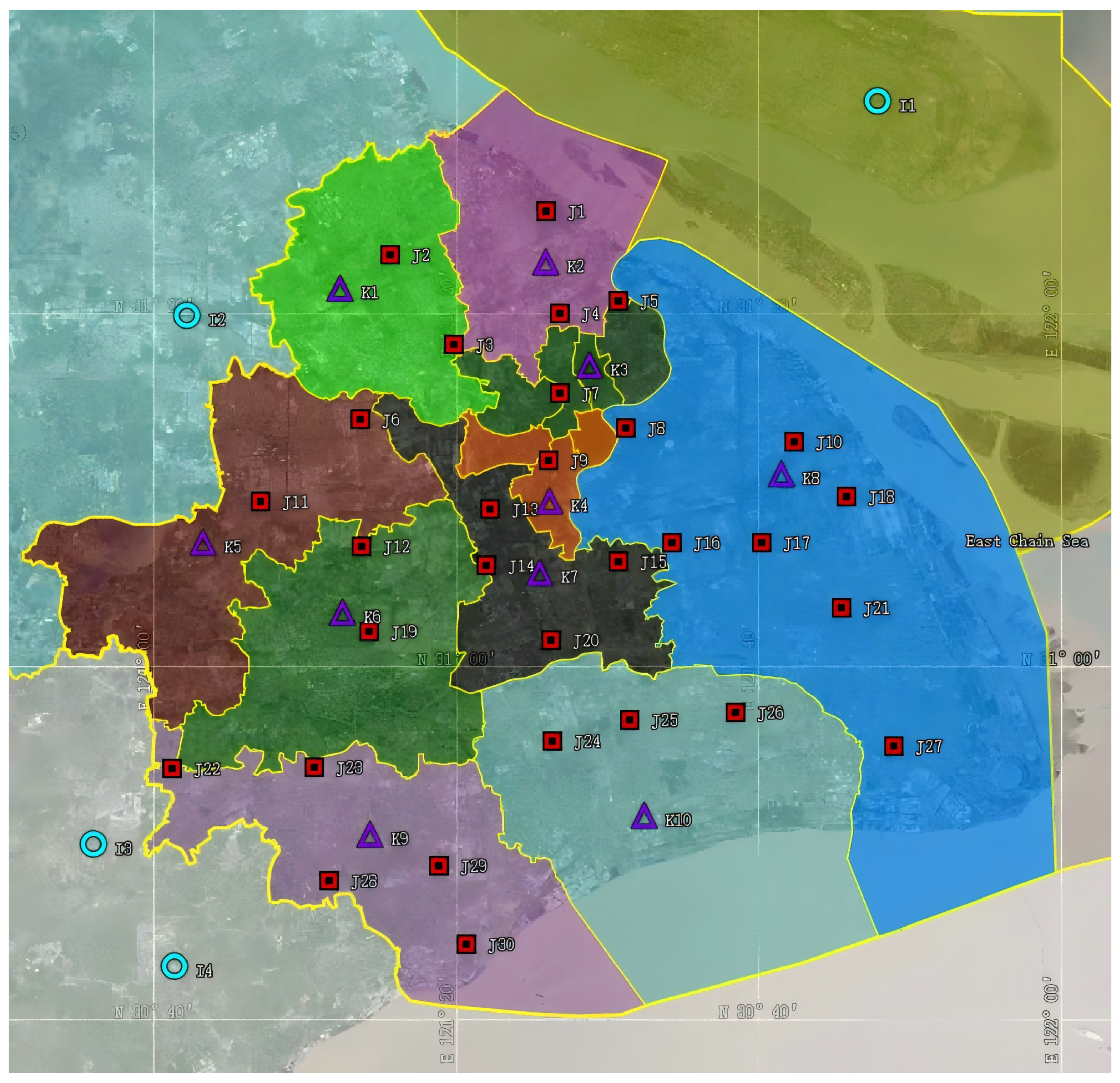
As the economy continues to grow, China’s new retail business model is experiencing rapid expansion. Take “Freshippo” as an example. Consumers who used to shop in supermarkets can now use the Freshippo app to buy all the commodities in the supermarket, so that they can enjoy the fun of shopping without going out to meet their needs. It can also be delivered quickly, taking 30 min to reach the customer’s door. The biggest difference from traditional fresh retail is that it uses big data to realize the optimal configuration of supply, distribution centers and customer distribution. Because of the particularity of fresh goods, it is necessary to carry out refrigerated transportation. How to choose the distribution center reasonably, reduce the storage cost and realize fast distribution to customers in time are problems worthy of further study. Take Shanghai’s fresh supply chain network as an example, in which fresh products are provided by four suppliers and distributed by 30 selectable distribution centers in order to meet the daily fresh demand of Freshippo consumers in 10 demand areas in Shanghai. The location relationship of the supply chain is shown in Figure 2. For the convenience of the discussion, we mark four suppliers, numbered from $I1$ to $I4$, and also mark the locations of 30 alternative distribution centers, numbered from $J1$ to $J30$, and 10 demand areas numbered from $K1$ to $K10$.

Demand area $K1$ is Jiading District. Demand area $K2$ is Baoshan District. Demand area $K3$ consists of Putuo District, Jing’an District, Yangpu District and Hongkou District. Demand area $K4$ consists of Changning District, Xuhui District and Huangpu District. Demand area $K5$ is Qingpu District. Demand area $K6$ is Songjiang District. Demand area $K7$ is Minhang District. Demand area $K8$ is Pudong New Area. Demand area $K9$ is Jinshan District. Demand area $K10$ is Fengxian District. Given that Chongming District is geographically isolated as an independent island, its consumption demand is excluded from the computational analysis.

To simplify the computational process, this study assumes a uniform price for fresh products. Furthermore, it is presumed that distribution centers are capable of successfully delivering fresh products to demand areas. The relevant parameters, random transportation costs and random demand are provided in

Table 1. Parameters for suppliers and distribution centers.

Index	Suppliers		Distribution	Centers
$I,J$	$a_i$	$b_i$	$d_j$	$e_j$
1	28,000	4.20	235	10,000
2	24,000	4.10	230	9480
3	26,000	4.40	220	9450
4	25,000	4.00	225	9470
5	/	/	240	9510
6	/	/	230	9490
7	/	/	245	9520
8	/	/	243	9505
9	/	/	233	9460
10	/	/	234	9485
11	/	/	233	9600
12	/	/	229	9380
13	/	/	219	9950
14	/	/	223	9770
15	/	/	238	9410
16	/	/	228	9800
17	/	/	243	9420
18	/	/	242	9600
19	/	/	223	9660
20	/	/	233	9600
21	/	/	243	9500
22	/	/	239	9320
23	/	/	219	9350
24	/	/	213	9370
25	/	/	226	9710
26	/	/	225	9500
27	/	/	213	9320
28	/	/	222	9500
29	/	/	223	9560
30	/	/	213	9400

,

Table 2. Expected costs of transportation from suppliers to distribution centers.

	I1	I2	I3	I4
$J1$	$0.35$	$0.35$	$0.40$	$0.41$
$J2$	$0.37$	$0.33$	$0.39$	$0.40$
$J3$	$0.36$	$0.34$	$0.38$	$0.39$
$J4$	$0.35$	$0.35$	$0.39$	$0.40$
$J5$	$0.34$	$0.36$	$0.40$	$0.40$
$J6$	$0.38$	$0.33$	$0.37$	$0.38$
$J7$	$0.36$	$0.35$	$0.38$	$0.39$
$J8$	$0.35$	$0.36$	$0.39$	$0.39$
$J9$	$0.36$	$0.35$	$0.38$	$0.38$
$J10$	$0.35$	$0.38$	$0.40$	$0.41$
$J11$	$0.40$	$0.33$	$0.35$	$0.36$
$J12$	$0.39$	$0.34$	$0.35$	$0.36$
$J13$	$0.37$	$0.35$	$0.37$	$0.37$
$J14$	$0.38$	$0.35$	$0.36$	$0.37$
$J15$	$0.37$	$0.37$	$0.38$	$0.38$
$J16$	$0.37$	$0.37$	$0.38$	$0.38$
$J17$	$0.36$	$0.38$	$0.40$	$0.39$
$J18$	$0.35$	$0.39$	$0.41$	$0.41$
$J19$	$0.39$	$0.35$	$0.35$	$0.35$
$J20$	$0.38$	$0.36$	$0.37$	$0.37$
$J21$	$0.37$	$0.39$	$0.40$	$0.40$
$J22$	$0.43$	$0.36$	$0.32$	$0.33$
$J23$	$0.41$	$0.36$	$0.33$	$0.33$
$J24$	$0.39$	$0.37$	$0.36$	$0.36$
$J25$	$0.39$	$0.38$	$0.37$	$0.37$
$J26$	$0.38$	$0.39$	$0.39$	$0.38$
$J27$	$0.38$	$0.41$	$0.40$	$0.40$
$J28$	$0.42$	$0.38$	$0.33$	$0.33$
$J29$	$0.41$	$0.38$	$0.35$	$0.34$
$J30$	$0.42$	$0.39$	$0.35$	$0.34$

,

Table 3. Expected costs of transportation from distribution centers to consumers.

	K1	K2	K3	K4	K5	K6	K7	K8	K9	K10
$J1$	0.33	0.31	0.32	0.34	0.36	0.36	0.35	0.35	0.38	0.38
$J2$	0.31	0.32	0.33	0.34	0.35	0.35	0.35	0.36	0.38	0.38
$J3$	0.32	0.32	0.32	0.33	0.34	0.34	0.33	0.35	0.37	0.37
$J4$	0.33	0.31	0.31	0.33	0.36	0.35	0.34	0.34	0.37	0.37
$J5$	0.34	0.31	0.31	0.33	0.36	0.35	0.34	0.33	0.38	0.37
$J6$	0.32	0.33	0.33	0.33	0.33	0.33	0.33	0.36	0.36	0.36
$J7$	0.33	0.32	0.31	0.32	0.35	0.34	0.33	0.33	0.36	0.36
$J8$	0.34	0.33	0.31	0.32	0.36	0.35	0.32	0.32	0.36	0.35
$J9$	0.34	0.33	0.32	0.31	0.35	0.34	0.32	0.33	0.36	0.35
$J10$	0.36	0.34	0.33	0.34	0.38	0.36	0.34	0.31	0.38	0.35
$J11$	0.33	0.35	0.35	0.34	0.31	0.32	0.34	0.37	0.35	0.37
$J12$	0.34	0.34	0.34	0.33	0.32	0.31	0.33	0.36	0.34	0.35
$J13$	0.34	0.34	0.33	0.31	0.34	0.33	0.31	0.34	0.35	0.35
$J14$	0.34	0.34	0.33	0.31	0.34	0.32	0.31	0.34	0.34	0.34
$J15$	0.35	0.34	0.33	0.31	0.35	0.34	0.31	0.33	0.35	0.34
$J16$	0.36	0.34	0.33	0.32	0.36	0.35	0.32	0.32	0.36	0.34
$J17$	0.36	0.35	0.33	0.33	0.37	0.36	0.33	0.31	0.36	0.34
$J18$	0.37	0.35	0.34	0.34	0.38	0.37	0.34	0.31	0.38	0.35
$J19$	0.35	0.35	0.35	0.33	0.33	0.31	0.33	0.36	0.33	0.35
$J20$	0.35	0.35	0.34	0.32	0.35	0.33	0.31	0.34	0.34	0.33
$J21$	0.38	0.36	0.35	0.34	0.38	0.37	0.34	0.32	0.33	0.36
$J23$	0.36	0.37	0.36	0.35	0.33	0.32	0.34	0.37	0.31	0.35
$J24$	0.37	0.36	0.35	0.33	0.35	0.33	0.32	0.35	0.33	0.32
$J26$	0.38	0.36	0.35	0.34	0.37	0.35	0.33	0.33	0.35	0.32
$J27$	0.39	0.38	0.36	0.36	0.39	0.38	0.35	0.34	0.37	0.34
$J28$	0.38	0.38	0.38	0.36	0.35	0.34	0.35	0.38	0.31	0.34
$J29$	0.38	0.38	0.37	0.35	0.35	0.34	0.34	0.37	0.31	0.33
$J30$	0.39	0.39	0.38	0.36	0.36	0.35	0.35	0.37	0.32	0.33

and

Table 4. Expected demand of consumer.

Consumer	K1	K2	K3	K4	K5
Expected demand	$8800-\varrho r$	$9000-\varrho r$	$10,000-\varrho r$	$9800-\varrho r$	$9100-\varrho r$
Consumer	K6	K7	K8	K9	K10
Expected demand	$9500-\varrho r$	$9700-\varrho r$	$9500-\varrho r$	$8700-\varrho r$	$8500-\varrho r$

.

Table 2 shows the expected costs of transportation from suppliers to distribution centers. Transportation costs primarily encompass fuel expenses, vehicle maintenance costs and driver salaries. The unit transportation cost is calculated using the following formula:

$$Fuelcost=distance\ast fuelconsumption\ast oilprice,$$

$$Unittransportationcost=fuelexpenses+vehiclemaintenancecosts+driversalaries.$$

For example, as shown in Table 2, to transport 1000 units of product from $I1$ to $J1$, the distance is 39 km, the fuel consumption is $12L/100$ km, the oil price is 9.93 CNY/L, the vehicle cost is CNY 100 and the engine cost is CNY 200. Because of this, the single-bit cost of transporting the raw materials is $(33\ast 12/100\ast 9.93+100+200)/1000=0.34$ CNY. Due to uncertain factors such as traffic congestion and traffic flow, we use CNY 0.35 to represent the first-moment information regarding the transportation cost from $I1$ to $J1$. Based on the above calculation rules, the first-moment information of random transportation costs is given in Table 2 and Table 3.

Based on market survey data, the daily online orders in Jiading District amount to 17,600 orders. Assuming that orders for fresh products at a uniform price constitute $50\%$ of the total, the expected demand for $K1$ is 8800. Through statistical analysis, the random daily consumer demand is as presented in Table 4, where $\varrho =10$ denotes the price elasticity coefficient of demand and r is set to CNY 12.

Since the random vectors are independent of each other, and according to the statistics of market survey data, the second moment (covariance matrix) satisfies $\sum =0.004\ast W$, where W is a 430-dimensional identity matrix. To solve the location assignment problem, for any feasible solution, we use the Monte Carlo method to generate 1000 scenarios, each generating 1000 random sampling points ${\xi }_n\left(\omega \right)$, $n=1,2,\cdots ,1000$, for random simulation (such a sample size is sufficient to simulate random expected values). When the data are generated, the first-order moment information is as shown in Table 2, Table 3 and Table 4, and the second-order moment satisfies $\sum =0.004\ast W$. The numerical results are shown in

Table 5. Numerical optimal solution and value of the example.

${\mathit{\beta }}^{*}=$	$(0,0,1,0,1,1,0,0,0,0,1,0,0,0,1,1,0,0,0,1,1,0,0,1,0,1,0,1,0,1)$
$x_{15}^{*}=9510.00$	$x_{1\underline{20}}^{*}=9600.00$	$x_{1\underline{21}}^{*}=4870.00$	$x_{1\underline{26}}^{*}=4020.00$	$x_{23}^{*}=9450.00$
$x_{26}^{*}=9490.00$	$x_{2\underline{15}}^{*}=430.00$	$x_{2\underline{21}}^{*}=4630.00$	$x_{3\underline{24}}^{*}=9370.00$	$x_{3\underline{30}}^{*}=5030.20$
$x_{4\underline{11}}^{*}=3730.00$	$x_{4\underline{16}}^{*}=9800.00$	$x_{4\underline{28}}^{*}=9500.00$	$x_{4\underline{30}}^{*}=1970.00$	$y_{33}^{*}=9450.00$
$y_{52}^{*}=249.90$	$y_{58}^{*}=9260.10$	$y_{65}^{*}=7860.00$	$y_{66}^{*}=1630.00$	$y_{\underline{11}6}^{*}=3730.00$
$y_{\underline{15}3}^{*}=430.00$	$y_{\underline{16}4}^{*}=9680.10$	$y_{\underline{16}8}^{*}=119.90$	$y_{\underline{20}2}^{*}=8020.10$	$y_{\underline{20}9}^{*}=1579.90$
$y_{\underline{21}5}^{*}=1120.00$	$y_{\underline{21}\underline{10}}^{*}=8380.00$	$y_{\underline{24}1}^{*}=8680.00$	$y_{\underline{24}2}^{*}=610.00$	$y_{\underline{24}7}^{*}=80.00$
$y_{\underline{26}6}^{*}=4020.00$	$y_{\underline{28}7}^{*}=9500.00$	$y_{\underline{30}9}^{*}=7000.10$	$Pro=622,280$	$val=-560,050$

,

Table 6. Results of the DSHGA with different parameters.

System		Parameters		Results
T	N	$P_c$	$P_m$	${\beta }^{*}$	Pro	Error (%)
200	500	0.9	0.05	$(0,1,0,1,0,1,1,1,1,0,1,1,0,1,0,$	$6.2019\times {10}^5$	0.34
				$0,1,1,0,0,1,1,0,0,1,0,0,1,0,1)$
500	500	0.9	0.05	$(0,0,1,0,1,1,0,0,0,0,1,0,0,0,1,$	$6.2210\times {10}^5$	0.03
				$1,0,0,0,1,1,0,0,1,0,1,0,1,0,1)$
1000	500	0.9	0.05	$(0,0,1,0,1,1,0,0,0,0,1,0,0,0,1,$	$6.2228\times {10}^5$	0.00
				$1,0,0,0,1,1,0,0,1,0,1,0,1,0,1)$
1000	100	0.9	0.05	$(0,0,1,0,1,1,0,0,0,0,1,0,0,0,1,$	$6.2216\times {10}^5$	0.02
				$1,0,0,0,1,1,0,0,1,0,1,0,1,0,1)$
1000	200	0.9	0.05	$(0,0,1,0,1,1,0,0,0,0,1,0,0,0,1,$	$6.2212\times {10}^5$	0.03
				$1,0,0,0,1,1,0,0,1,0,1,0,1,0,1)$
1000	300	0.9	0.05	$(0,0,1,0,1,1,0,0,0,0,1,0,0,0,1,$	$6.2216\times {10}^5$	0.02
				$1,0,0,0,1,1,0,0,1,0,1,0,1,0,1)$
1000	500	0.92	0.05	$(0,0,1,0,1,1,0,0,0,0,1,0,0,0,1,$	$6.2223\times {10}^5$	0.01
				$1,0,0,0,1,1,0,0,1,0,1,0,1,0,1)$
1000	500	0.94	0.05	$(0,0,1,0,1,1,0,0,0,0,1,0,0,0,1,$	$6.2215\times {10}^5$	0.02
				$1,0,0,0,1,1,0,0,1,0,1,0,1,0,1)$
1000	500	0.96	0.05	$(0,0,1,0,1,1,0,0,0,0,1,0,0,0,1,$	$6.2220\times {10}^5$	0.01
				$1,0,0,0,1,1,0,0,1,0,1,0,1,0,1)$
1000	500	0.9	0.02	$(0,0,1,0,1,1,0,0,0,0,1,0,0,0,1,$	$6.2218\times {10}^5$	0.02
				$1,0,0,0,1,1,0,0,1,0,1,0,1,0,1)$
1000	500	0.9	0.07	$(0,0,1,0,1,1,0,0,0,0,1,0,0,0,1,$	$6.2215\times {10}^5$	0.02
				$1,0,0,0,1,1,0,0,1,0,1,0,1,0,1)$

,

Table 7. Comparisons of different algorithms.

Algorithm	${\mathit{\beta }}^{\mathbf{*}}$	Pro	Fit	TI
DSHGA	$(0,0,1,0,1,1,0,0,0,0,1,0,0,0,1,$	$6.2228\times {10}^5$	$5.6005\times {10}^5$	$36937.3489$
	$1,0,0,0,1,1,0,0,1,0,1,0,1,0,1)$
Liu [26]	$(0,0,1,0,1,1,0,0,0,0,1,0,0,0,1,$	$6.2223\times {10}^5$	$5.6003\times {10}^5$	$38235.7439$
	$1,0,0,0,1,1,0,0,1,0,1,0,1,0,1)$

,

Table 8. Supply chain location and profit under different optimization models.

Algorithm	${\mathit{\beta }}^{*}$	Pro	Fit
No-Risk ($\lambda =1$)	$(0,1,0,1,1,1,1,1,1,0,1,1,1,1,1,$	$6.2309\times {10}^5$	$6.2309\times {10}^5$
	$1,1,0,0,0,1,0,1,0,0,0,0,1,1,0)$
SVaR	$(0,0,1,0,1,1,0,0,0,0,1,0,0,0,1,$	$6.2228\times {10}^5$	$5.6005\times {10}^5$
	$1,0,0,0,1,1,0,0,1,0,1,0,1,0,1)$
VaR	$(0,0,1,1,0,0,1,1,1,0,0,0,0,0,1,$	$6.2179\times {10}^5$	$5.5553\times {10}^5$
	$0,0,1,0,1,1,1,0,0,1,1,0,1,1,0)$

and

Table 9. Supply chain profit with robustness and no robustness.

Algorithm	${\mathit{\beta }}^{*}$	Pro	Fit
No-Robust	$(0,1,0,1,1,1,0,1,1,0,1,1,1,0,1,$	$6.2286\times {10}^5$	$5.6921\times {10}^5$
	$1,1,0,0,0,1,0,1,0,0,0,0,1,1,0)$
Robust	$(0,0,1,0,1,1,0,0,0,0,1,0,0,0,1,$	$6.2228\times {10}^5$	$5.6005\times {10}^5$
	$1,0,0,0,1,1,0,0,1,0,1,0,1,0,1)$

and Figure 3, Figure 4 and Figure 5, respectively.

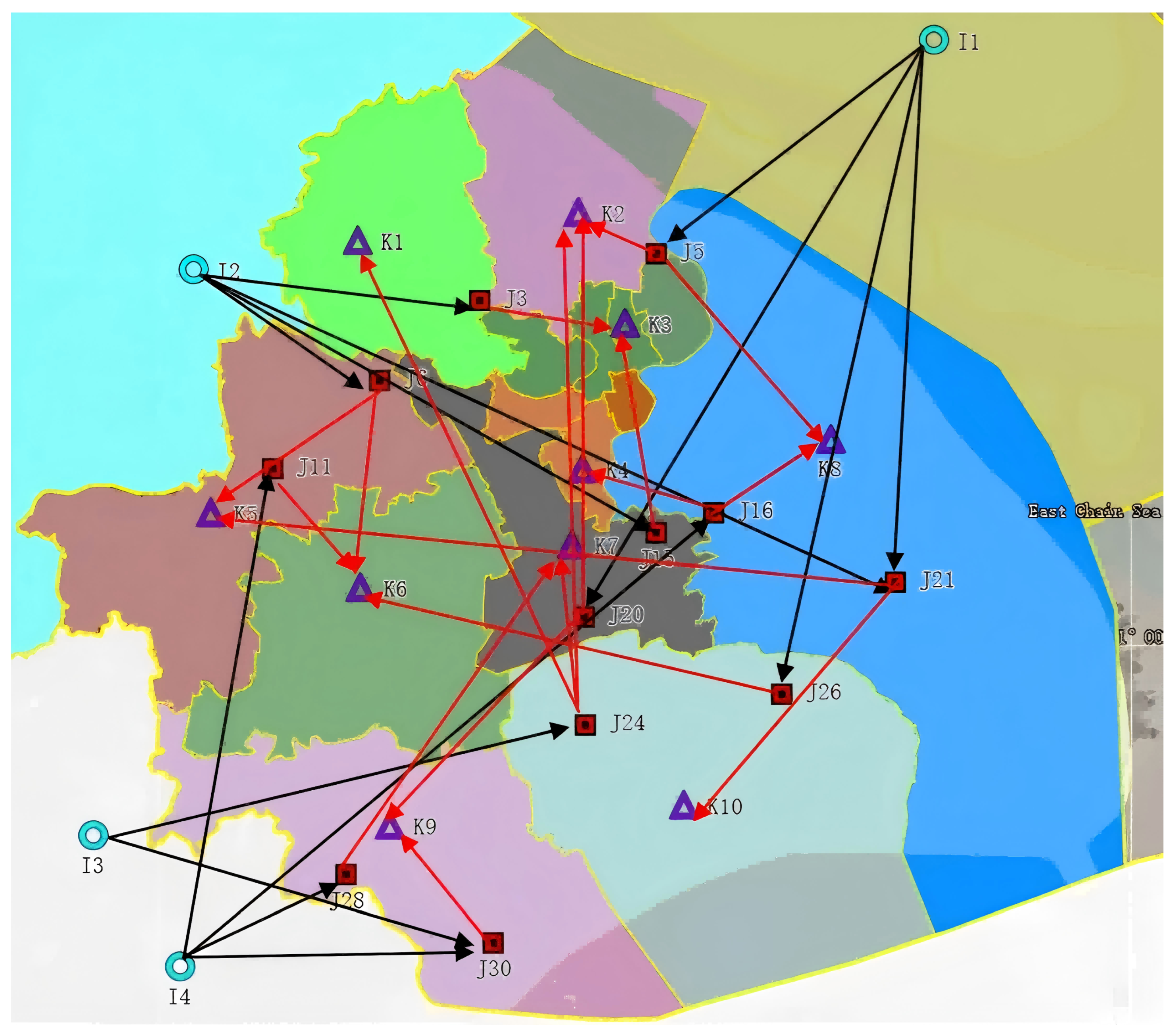
Figure 3 illustrates the supply chain network for location allocation, with detailed results presented in Table 5. To maximize customer satisfaction, the enterprise selects $J3$, $J5$, $J6$, $J11$, $J15$, $J16$, $J20$, $J21$, $J24$, $J26$, $J28$ and $J30$ as distribution centers to supply fresh products to customers. Under this configuration, the supply chain achieves a maximum profit of CNY $6.2228\times {10}^5$. The expected demand of demand area $K1$ is $E\left[K1\right]=8800-\varrho r=8680.00$, and the distribution is completed by distribution center $J24$. The expected demand of demand area $K2$ is $E\left[K2\right]=9000-\varrho r=8880.00$, which is provided by $J5$, $J20$ and $J24$, with $249.90$, $8020.10$ and $610.00$, respectively The expected demand of demand area $K3$ is $E\left[K3\right]=10000-\varrho r=9880.00$, which is provided by $J3$ and $J15$, with $9450.00$ and $430.00$, respectively. The expected demand of demand area $K4$ is $E\left[K4\right]=9800-\varrho r=9680.00$, and the distribution is completed by distribution center $J16$. The expected demand of demand area $K5$ is $E\left[K5\right]=9100-\varrho r=8980.00$, which is provided by $J6$ and $J21$, with $7860.00$ and $1120.00$, respectively. The expected demand of demand area $K6$ is $E\left[K6\right]=9500-\varrho r=9380.00$, which is provided by $J6$, $J11$ and $J26$, with $1630.00$, $3730.00$ and $4020.00$, respectively. The expected demand of demand area $K7$ is $E\left[K7\right]=9700-\varrho r=9580.00$, which is provided by $J24$ and $J28$, with $80.00$ and $9500.00$, respectively. The expected demand of demand area $K8$ is $E\left[K8\right]=9500-\varrho r=9380.00$, which is provided by $J5$ and $J16$, with $9260.10$ and $119.90$, respectively. The expected demand of demand area $K9$ is $E\left[K9\right]=8700-\varrho r=8580.00$, which is provided by $J20$ and $J30$, with $1579.90$ and $7000.10$, respectively. The expected demand of demand area $K10$ is $E\left[K10\right]=8500-\varrho r=8380.00$, and the distribution is completed by distribution center $J21$. At the same time, it can be seen from Figure 3 that the location of the selected distribution center is relatively close to the suppliers and demand areas, meeting the principle of nearby supply.

To further demonstrate the effectiveness of the DSHGA, we evaluate its stability by varying the number of iterations, population size and parameter settings. The numerical outcomes are presented in Table 6, with the final column indicating the relative error, defined as follows:

$$Error={\displaystyle \frac{OptimalPro-Pro}{OptimalPro}}\times 100\%.$$

As shown in Table 6, varying the iterations, population sizes and parameters in the DSHGA results in relative errors not exceeding $0.34\%$, demonstrating that the DSHGA exhibits strong parameter robustness and is capable of effectively addressing the two-stage distributionally robust mean semi-variance mixed-integer optimization problem. Furthermore, the observed relative error arises from the use of the Monte Carlo method for random simulation during the computational process.

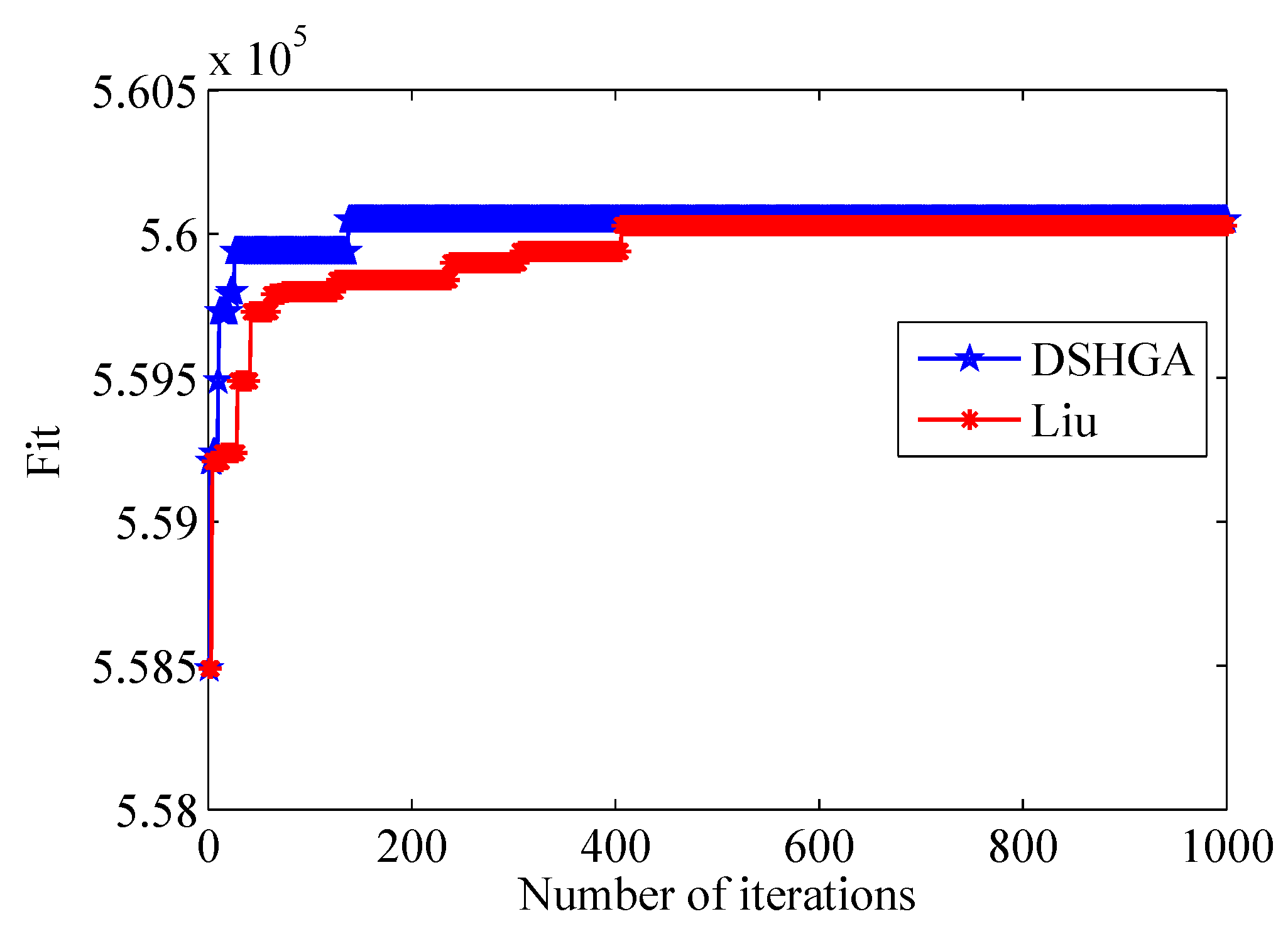
To further assess the efficacy of our proposed DSHGA, a comparative analysis is conducted against other discrete hybrid optimization techniques, including the GA developed by Liu [26]. The comparative performance metrics are presented in Table 7, while the corresponding graphical representation of the results is illustrated in Figure 4.

As demonstrated in Table 7, the implementation of two distinct algorithmic approaches for addressing the supply chain location allocation problem yields identical optimal solutions. Notably, the application of the DSHGA exhibits superior performance characteristics, achieving maximal supply chain profitability while concurrently demonstrating enhanced computational efficiency through reduced processing time. As can be seen from Figure 4, the algorithm proposed in this paper converges faster than the algorithm proposed by Liu [26], and it can be considered that the DSHGA is more suitable for solving this problem.

In Table 8, we compare the impact of three optimization models on decision-making and profit when modeling the supply chain. The examined models include (1) a two-stage distributionally robust mixed-integer optimization model $(\lambda =1)$, (2) a two-stage distributionally robust mean semi-variance mixed-integer optimization model and (3) a two-stage distributionally robust mean variance mixed-integer optimization model incorporating Value at Risk (VaR) as the risk measurement function. The computational results reveal distinct patterns in supply chain profitability under varying risk considerations. The baseline scenario, excluding risk factors, yields a supply chain profit of $6.2309\times {10}^5$. Incorporation of the SVaR metric results in a marginally reduced profit of $6.2228\times {10}^5$, demonstrating that risk-adjusted profitability metrics exhibit more conservative estimates compared to risk-neutral scenarios, aligning with empirical observations. Furthermore, the implementation of VaR as the risk measure generates a profit of $6.2179\times {10}^5$, representing a $0.08\%$ reduction relative to the SVaR-based model. This comparative analysis suggests that the SVaR metric provides a more accurate representation of risk perception than the conventional VaR approach. Regarding Model (1), sensitivity analysis indicates that the $\lambda$ exerts significant influence on decision-making outcomes. Strategic adjustment of the SVaR weighting coefficient enables decision-makers to achieve targeted benefit expectations. 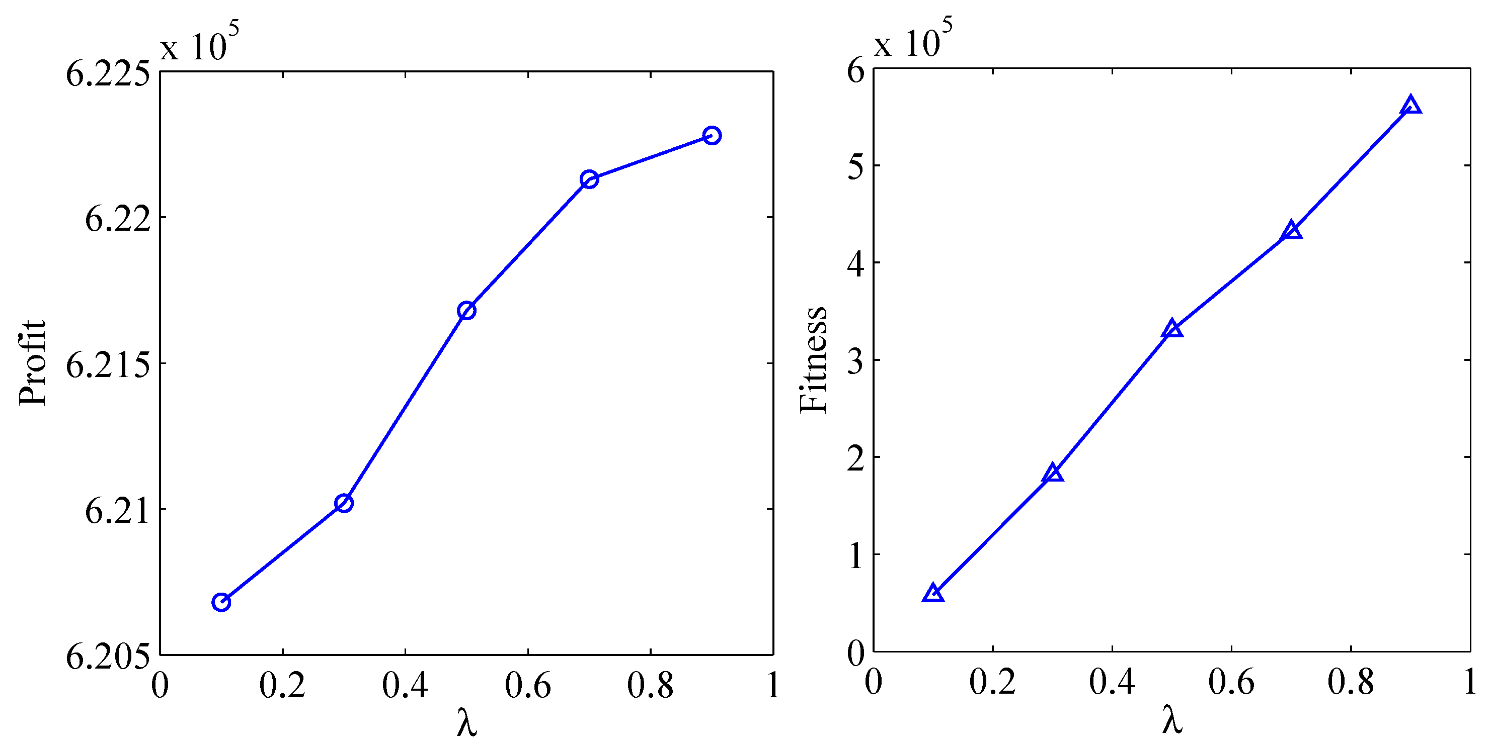The quantitative impact of $\lambda$ variations on both supply chain profitability and objective function values is systematically presented in Figure 5.

As can be seen from Figure 5, when $\lambda$ increases from $0.1$ to $0.9$, the corresponding risk weight $(1-\lambda )$ decreases from $0.9$ to $0.1$, the supply chain profit increases, the corresponding fitness function value increases and the function value Val = −Fit decreases. In other words, the greater the risk weight $(1-\lambda )$, the more conservative the decision will be. In the uncertain environment, the decision-maker can consider the corresponding risk weight according to the actual situation and make the optimal decision.

Table 9 shows the optimal location, profit and function values of the supply chain under the worst-case and expected scenarios. The computational results demonstrate significant divergence in optimal decision-making outcomes between these two scenario frameworks. In the worst-case scenario, the supply chain achieves a conservative profit margin of CNY $6.2228\times {10}^5$, accompanied by correspondingly conservative location decisions. This conservative configuration ensures solution feasibility across the entire uncertainty set, thereby demonstrating the model’s inherent robustness against parameter variations. Conversely, the expected scenario yields an enhanced profitability of CNY $6.2286\times {10}^5$. However, while this scenario presents superior expected returns compared to the robust optimization approach, it potentially overestimates achievable outcomes, presenting an optimistic bias that may not accurately reflect real-world operational conditions. The comparative analysis underscores the fundamental trade-off between solution robustness and optimality in supply chain optimization under uncertainty. Moreover, it is difficult to predict the exact probability distribution in practice. Therefore, in the absence of precise probabilistic information about uncertainty, the decision-maker can formulate a robust plan using a two-stage distributionally robust mixed-integer optimization model.

Management insights

This study develops a data-driven two-stage distributionally robust mean semi-variance mixed-integer optimization model with the following distinctive features:

(a)

Simultaneous consideration of transportation cost volatility and customer demand uncertainty;

(b)

Incorporation of SVaR as a risk measure for cost functions;

(c)

Application of distributionally robust mixed-integer programming to ensure implementable solutions.

Compared with traditional risk-neutral approaches, our risk-averse model demonstrates three key advantages:

(a)

It effectively captures volatility in uncertain outcomes;

(b)

It provides more reliable decision support in uncertain environments;

(c)

It enables flexible strategy adjustment based on risk preferences.

The data demonstrate that decision-makers can flexibly adjust the SVaR weighting parameter based on their risk preferences to achieve an optimal balance between expected returns and risk protection, as detailed in Table 8 and Figure 5.

Comparative analysis through the models shows the following:

(a)

The results of the distributionally robust model are relatively conservative, but ensure feasibility in all scenarios;

(b)

Although non-robust models show higher expected profits, there is a significant optimistic bias (see Table 9 for specific numerical comparisons).

Based on the above analysis, we derive some managerial insights. This method enables decision-makers in complex supply chain environments to carry out the following:

(a)

Quantitatively evaluate the risk–return characteristics of different strategies;

(b)

Avoid operational risks caused by over-optimistic estimations;

(c)

Obtain uncertainty-resilient decision solutions.

This study provides a new methodological tool for supply chain risk management, particularly suitable for the current highly volatile business environment. Decision-makers can find the optimal balance between the robustness of the plan and the expected returns based on their actual risk tolerance.

7. Conclusions

This study addresses the location allocation optimization problem under conditions of uncertain transportation costs and demand fluctuations through the development of a novel two-stage distributionally robust mean semi-variance mixed-integer optimization framework. The proposed model, constructed using a data-driven methodology, incorporates an uncertainty set encompassing all probability distribution functions that equal the first and second moments. Compared with the traditional stochastic optimization model, the model is more robust in numerical simulation. Considering the complexity of the model, a DSHGA is proposed to solve the model. Compared with other algorithms, the effectiveness of the algorithm is illustrated by the calculation time, iteration steps and convergence speed.

It is particularly noteworthy that the proposed model in this study exhibits significant versatility, being not only applicable to conventional location allocation problems but also extendable to complex joint optimization scenarios, including emergency resource distribution and integrated production–inventory–transportation systems. The construction of uncertainty sets is the key when employing distributionally robust optimization frameworks for supply chain optimization problems. Beyond the moment-based constraint approach adopted in this work, alternative uncertainty set formulations can be developed through statistical measurement theories. Specifically, the Wasserstein distance provides a robust metric for quantifying distributional differences between empirical and reference probability distributions. Such distributions can be effectively estimated through data-driven approaches incorporating nonparametric estimation techniques, representing a valuable direction for future research endeavors. This study also has some limitations. For instance, when constructing the uncertainty set, incomplete historical data or excessive noisy data may lead to an incomplete uncertainty set or data bias. In such cases, machine learning algorithms such as clustering algorithms, deep learning algorithms and statistical learning algorithms can be incorporated to construct the uncertainty set, which also provides a valuable direction for future research.