Abstract
The ground-based real aperture radar (GB-RAR), with its non-contact, high-precision, continuous monitoring capabilities, is widely used in bridge safety. To reduce noise interference in GB-RAR monitoring, a denoising method based on complementary ensemble empirical mode decomposition (CEEMD), wavelet threshold denoising (WTD), and principal component analysis (PCA) was applied to the safety monitoring of the East Lake High-tech Bridge in Wuhan. The method involved CECEEMD of GB-RAR data, WTD for high-frequency noise Intrinsic Mode Function (IMF) components, and PCA for low-frequency IMF power spectrum matrices to remove coloured noise. PCA shows a symmetric balance between noise removal and signal retention. The experimental results show that the proposed denoising method ensures the integrity of the reconstructed signal by symmetrically processing the IMF of high and low frequencies and improves the signal-to-noise ratio (SNR) of the three piers to 8.30, 19.87 and 15.06, respectively, and the Root Mean Square Errors (RMSE) are 0.10 mm, 0.06 mm and 0.09 mm, respectively. Noise removal reduced uncertainty by 42.3%, 35.8%, and 33.1%, demonstrating the method’s effectiveness in enhancing deformation monitoring precision.
1. Introduction
As transportation networks continue improving, connections between regions become increasingly intertwined. Transport infrastructure, such as bridges, bolsters economic, cultural, and social exchanges between shores or territories. The completion and utilization of the Hong Kong–Zhuhai–Macao Bridge (HZMB) has injected vigorous impetus into the take-off of the Guangdong–Hong Kong-Macao Greater Bay Area, and communication among the three places has become increasingly frequent.
However, due to lifespan, load effects, and geological activities, bridges inevitably face oxidation, wear, and degradation issues. These challenges can alter the structural stability of bridges, increasing the risk of incidents. Therefore, when designing bridges, it is essential to consider the environment being used and select durable materials, ensuring both the safety and longevity of the bridge. Moreover, once a bridge is operational, regularly monitoring its deformations is vital to understanding its dynamic characteristics, which is crucial for its construction and safe operation [1].
The deformation data monitoring methods used in bridges today include the Global Navigation Satellite System (GNSS) technique [2,3], sensor methods [4], and other techniques [5,6,7]. Ruijie Xi et al. used multi-GNSS observations with a high cutoff height and proposed a multi-GNSS integrated processing algorithm to achieve deformation monitoring of the Yangtze River Bridge in Wuhan Baishazhou. The results not only counterbalanced the problem observations of low satellite elevation angle but also extracted more accurate displacement and vibration signals of the bridge. Miguel A. Vicente et al. used a new laser and a video-based displacement sensor (LVBDT) to monitor displacement and rotation in the Loiola Station Bridge structure in the city of San Sebastián, Spain, and demonstrated the feasibility of the proposed method through laboratory experiments and field tests. Many current methods use contact sensors to monitor deformations at fixed characteristic points on bridges. While this allows for insight into local deformation patterns, it does not facilitate concurrent monitoring of the bridge’s overall state. Additionally, installing these monitoring systems is time-intensive, and each instrument is typically designed for a singular measurement task, limiting efficiency. The GB-RAR [8,9,10] represents a novel non-contact monitoring technology. With benefits such as high spatial and temporal resolution, ease of station setup, exceptional accuracy, and expansive coverage, GB-RAR has found extensive applications in the dynamic monitoring of buildings. Hu [11] used GB-RAR to monitor a bridge’s deflection changes and modal parameters. They combined GNSS with GB-RAR for resonance frequency monitors in bridge health monitoring, and the results of the two methods were highly consistent. Kuras [12] utilized GB-SAR to safely monitor a large-span tram overpass in Poland, demonstrating the portability and efficiency of GB-SAR monitoring compared to traditional measurement means. Gao [13] used a vector network analyzer to construct a ground-based interferometric radar system that transmits step-frequency continuous wave signals to monitor bridge deflection and then analyze the dynamic coefficient, deflection ratio, damping ratio, and other parameters. Finally, they compared and analyzed the simulation results with the measured results of the ground-based interferometric radar to prove the accuracy and effectiveness of the ground-based interferometric radar in bridge monitoring applications.
During bridge deformation monitoring via GB-RAR, external environmental factors and human observational influences can introduce noise into the monitoring data. This introduces uncertainties, manifested as data mutation and spikes, that hinder the extraction of vital monitoring information and subsequent deformation analysis. Analyses of monitoring data reveal the presence of not just white noise but also coloured noise. White noise refers to random noise whose power spectrum is uniformly distributed over all frequency ranges, usually caused by measurement errors or instrument electronic noise, and is mainly presented as high-frequency signals; while coloured noise is time-dependent, whose power spectrum varies with frequency, usually caused by environmental factors or structural influences, and is mainly presented as low-frequency signals. In bridge monitoring, white noise is often considered to be random interference, while colour noise may contain information related to changes in bridge structure. If coloured noise is mistreated as white noise, bridge deformation may be misassessed and the quality of monitoring data may be reduced [14]. The coloured noise is more likely to affect the bridge monitoring data due to its non-stationary and interrelated characteristics, as opposed to the white noise’s independent and uniformly distributed characteristics. In order to improve the reliability and rigour of the algorithm in this paper, a bridge deformation monitoring system capable of accurately identifying and filtering noise is established, so the effects of colour noise are also considered when dealing with white noise. As such, while addressing white noise, it is imperative to mitigate the effects of coloured noise [15,16,17]. Conventional denoising techniques for monitoring data encompass filtering methods [18], empirical mode decomposition (EMD), and wavelet thresholding denoising. Filtering methods enhance the signal-to-noise ratio (SNR) by targeting noise with specific traits. However, their efficacy demands information about the data or noise characteristics. As such, without detailed monitoring data characterization, these methods struggle with bridge data exhibiting non-smooth traits. EMD has good results in decomposing nonlinear non-smooth data. As an adaptive decomposition technique [19,20], EMD dissects data into Intrinsic Mode Function (IMF) [21], from high to low-frequency. This negates the need for defining the basis function or number of decomposition layers, providing time-frequency localization and adaptive decomposition. The EMD denoising approach emphasizes removing high-frequency noise from the IMF components, yet neglects coloured noise at low frequencies. Complementary ensemble empirical model decomposition (CEEMD) is an improved algorithm proposed by Yeh [22] based on EMD followed by EEMD [23,24,25]. CEEMD enhances the decomposition efficiency by adding an auxiliary white noise of the two original data with opposite numbers to each other, which cancels out during ensemble averaging and consequently cancels out the ensemble counts. However, CEEMD may produce some residual noise during the decomposition process, especially in high-order IMF, so it still can not achieve the ideal effect of denoising. Wavelet threshold denoising techniques [26,27] are capable of removing high-frequency noise while preserving critical deformation information, avoiding the issue of excessive signal smoothing, and are widely used in the processing of nonlinear, non-stationary signals. Still, WTD’s predominant focus is on the effects of white noise during wavelet decomposition, rendering them adept at eliminating high-frequency Gaussian white noise but less effective against low-frequency coloured noise. Ren Ankang [28] introduced a time-domain data extraction method for the GNSS displacement time series that accounts for coloured noise. Yet, before data processing, one must discern the optimal noise model for subsequent modelling, a labour-intensive task. Abdullah, H.A [29] used the CEEMD-WTD combinatorial algorithm to process the signal of the Impact-Type Sunflower Yield Sensor and successfully removed the non-smoothing random signal of the sensor’s output signal, demonstrating the superiority of CEEMD and WTD in comparison with other relevant denoise reduction algorithms. Liu Xianglei [30] applied a high-frequency denoising approach merged with the wavelet synchro-squeezing transform (WSST) method with the extreme point symmetric mode decomposition (ESMD) method to counteract the high-frequency noise in GB-SAR monitoring data. This method largely preserved high-frequency IMF information but overlooked low-frequency noise. Traditional wavelet or mean filtering methods, when dealing with low-frequency noise, often result in the loss of some signal components. In contrast, PCA, by performing principal component analysis on the power spectrum matrix, removes only the coloured noise components with minor contribution, which can effectively preserve the overall trend of the signal, making the denoised signal more consistent with the actual deformation characteristics. Based on this issue, Hamza Ahsan Abdullah and others used complete ensemble empirical mode decomposition with adaptive noise (CEEMDAN) to process the deformation data of a vibrating bridge, extracting Intrinsic Mode Functions (IMF) for signal reconstruction. After removing high-frequency noise through Empirical Wavelet Transform (EWT), they particularly introduced Kernel principal component analysis (KPCA) to effectively compress and project the spectral centroid feature matrix, further mitigating the impact of low-frequency noise and enhancing the quality of the monitoring data.
In summary, while considerable research has been undertaken on monitoring data denoising with numerous findings [31,32,33], there is a lack of studies on the coloured and white noise in the monitoring data of GB-RAR bridges monitoring data simultaneously. Therefore, this study applies the CEEMD-WTD method to denoise the GB-RAR bridge monitoring data and combines PCA to further optimize the removal of low-frequency coloured noise in order to improve monitoring accuracy and ensure the long-term reliability of the data. Compared to the existing CEEMD-WTD methods, the main innovations of this study include the following: (1) optimizing the denoising strategy for the noise characteristics of GB-RAR data, where after CEEMD signal decomposition, WTD is used to process high-frequency white noise, and PCA is combined to further remove low-frequency coloured noise, ensuring the integrity and precision of the signal; (2) calculating the power spectral matrix of the GB-RAR monitoring data through PCA, and based on the inverse Fourier transform, identifying and removing low-frequency coloured noise, addressing the issue that traditional methods struggle to separate low-frequency trend noise. Experimental outcomes affirm that the integrated CEEMD-WTD approach more adeptly retains data characteristics. Compared to the standalone WTD method [34,35], it exhibits improved SNR and reduced RMSE. Furthermore, PCA diminishes the deformation trend of low-frequency noise post central component removal, minimizing the coloured noise’s interference with monitoring data.
2. Methodology
2.1. Principles of the CEEMD Method
Due to the modal aliasing problem in EMD processing of monitoring data, it brings additional difficulties in interpretation. Wu [36] added white noise to the original data to overcome the problem of modal aliasing. However, the white noise will have a residual after the decomposition computation, indirectly increasing the calculation and error. CEEMD maintains the advantages of both while solving the problems of mode aliasing in EMD and significant reconstruction error in EEMD. The following are the steps of the CEEMD algorithm [37,38,39]:
Step 1: Two sets of Gaussian white noise, , with opposite signs added to the original signal, , resulting in two sets of noisy signals, represented as the following:
In the formula, represents the i-th set of Gaussian white noise, while and denote the signals after adding positive and negative noise, respectively.
Step 2: EMD was sequentially applied to the noisy signals and , and the j-th IMF component from each decomposition was obtained, denoted as and .
Step 3: The IMF components from all n groups were averaged to obtain the final expression of the j-th IMF component as follows:
In the formula, denotes the final averaged j-th IMF component.
Step 4: All IMF components are summed with the residual term to reconstruct the original signal :
2.2. Wavelet Thresholding Denoising
The wavelet threshold denoising method has good effects on the suppression of high-frequency white noise [40]. However, since the traditional wavelet denoising method is only designed for Gaussian white noise, and GB-RAR monitoring data contain both white noise and coloured noise, the sole use of the wavelet threshold denoising (WTD) method is difficult to effectively remove low-frequency coloured noise. Therefore, in this paper, after CEEMD, the WTD method is applied only to the high-frequency IMF components, ensuring that the main components of the signal are not mistakenly deleted.
The model for a one-dimensional noisy signal can be represented as follows:
where denotes the data containing noise; is the actual data; is the noise sequence; is the noise amplitude coefficient. By performing a discrete wavelet transform in Equation (6):
where is the wavelet coefficient, is the wavelet basis function. The Mallat algorithm calculates the following:
where and are the low-pass and high-pass filters, respectively. Then, the wavelet reconstruction formula is as follows:
where and are the reconstruction filters. The discrete wavelet coefficients are the following:
where is the wavelet coefficient of the true signal, and is the wavelet coefficient of the noise.
In summary, the wavelet transform separates the actual data in the noisy data according to the characteristic that the wavelet coefficients of the data differ from the wavelet coefficients of the noise [41,42].
2.3. CEEMD-WTD-Based Denoising Method
The CEEMD denoising method is based on decomposing the monitoring signal into adaptive IMF components with different frequencies and unequal bandwidths from high frequency to low frequency. Then, according to the characteristic that white noise is generally distributed in the high-frequency IMF component, the denoised bridge monitoring data are obtained by judging the demarcation point between the high-frequency IMF component and the low-frequency IMF component and reconstructing the low-frequency IMF and the trend term in addition to the high-frequency IMF component. However, the removal of all high-frequency IMF components may result in excessive denoising, ignoring the valuable data in the high-frequency noise, leading to different degrees of distortion of the original data, failing to retain the characteristic morphological information of the monitoring data, and, thus, affecting the subsequent data processing and analysis. When WTD is combined with CEEMD, it can accurately denoise high-frequency IMF components after CEEMD, effectively avoiding modal aliasing and improving denoising stability. The method proposed in this study is the CEEMD-WTD method, which denoises the noisy data by finding the demarcation point between the noise IMF components and the information IMF components through energy entropy. Energy entropy is concerned with the energy share of the monitoring data. In the CEEMD of the monitoring data to obtain multiple IMF components, each IMF component represents a different scale and frequency component of the signal, and the energy entropy describes the energy distribution of each layer of IMF in the monitoring data. As the energy entropy value of an IMF increases, it indicates a more dispersed energy distribution within that IMF component, leading to a lower energy proportion in the original monitoring data. Conversely, a smaller IMF component energy entropy value suggests a more concentrated energy distribution, resulting in a higher energy proportion within the original data. The CEEMD-WTD method is to overcome the disadvantages of single CEEMD and WTD but also maintain the advantages of both and improve the monitoring accuracy. The specific steps are as follows:
Step 1: The data with coloured noise removed is subjected to CEEMD to obtain the IMF components from high to low frequencies in order.
Step 2: For each IMF component , its energy was calculated, followed by the computation of its energy ratio and energy entropy . The specific formulas are as follows:
Component energy calculation:
where is the i-th IMF component, and is the total length of the signal.
Total energy calculation:
where is the total number of IMF components.
Energy ratio calculation:
where represents the proportion of the i-th IMF component in the total energy .
Energy entropy calculation:
Energy entropy reflects the complexity of the information carried by the IMF component and is commonly used to identify noise components.
Step 3: Wavelet threshold denoising was applied to the IMF components identified as noise.
Step 4: Reconstituting WTD denoised data with unprocessed IMF components into new denoised data.
2.4. Principal Component Analysis and Data Reconstruction
The CEEMD-WTD algorithm has been preliminarily implemented in previous signal processing and has achieved tremendous success. Although the algorithm greatly reduces high-frequency noise, it is unable to remove the low-frequency noise that remains in the residual signal, which is also a deficiency of the CEEMD-WTD algorithm. In view of this, this paper innovatively proposes the use of PCA to process and obtain the principal components of the coloured noise power spectrum, then, through inverse Fourier transform, obtain the coloured noise time series and remove it from the original monitoring data. Finally, reconstructing each IMF component results in the reconstructed denoised signal. When GB-RAR performs high-frequency pattern monitoring of bridges, the monitored displacement time series will contain not only white noise but may also contain time-correlated coloured noise. Whereas the two differ in their power spectrum, the power spectrum of coloured noise is a function of frequency and has different magnitudes of energy at different frequencies [43]. The power spectrum of white noise is constant and has equal energy at all frequencies. In this study, based on the differences in the power spectra between coloured noise and white noise, PCA is applied to process the power spectrum of the GB-RAR monitoring data to extract the principal components of the coloured noise power spectrum. By reconstructing the coloured noise sequence from these components, it can then be subtracted from the original monitoring data, effectively removing the coloured noise.
Step 1: Power spectrum calculation of the GB-RAR monitoring data for the three piers. The power spectrum curve changes smoothly by taking the logarithm of the frequency and power with a base of 10. Then, the logarithmic power spectrum of the three piers forms the matrix , , which is the logarithmic power spectrum of the displacement time series of piers 6, 7, and 8, respectively.
Step 2: Normalize the power spectrum. The composition of the power spectrum matrix is followed by the normalization of each power spectrum to prevent a power spectrum with too large a value from dominating the subsequent principal component analysis and thus neglecting the other principal components.
We normalized each power spectrum within the matrix to ensure that ranges with disproportionately large values do not overshadow subsequent principal component analyses, preserving the relevance of other main components.
where is the element in row , column of the power spectrum after normalization, , is the number of observations. is the number of bridge piers, where . is the row and column element of the matrix . and are the mean and standard deviation of the power spectrum of the b-th column of the matrix , respectively.
Step 3: Find the eigenvalues according to the power spectrum matrix, and with the eigenvector matrix , arrange the eigenvalues in descending order of numerical magnitude, and is the eigenvector corresponding to .
Step 4: Calculate the principal components and reconstruct the coloured noise power spectrum. The formula is as follows:
where , is the i-th principal component, and is the eigenvector matrix. The cumulative contribution is calculated to determine the principal component of coloured noise. GB-RAR monitoring data affected by coloured noise will have a higher proportion of coloured noise than white noise and, therefore, may contain coloured noise in the first and second principal components of the power spectrum obtained from principal component analysis.
After normalizing the power spectrum of the coloured noise, we reconstructed the data by taking the first and second principal components from the given equation.
where , is then inversely normalized to obtain the logarithmic power spectrum of the coloured noise at the three piers .
is the recovered power spectral value, and is an element in the reconstructed principal component matrix.
Step 5: Perform the Fourier inverse variation on the reconstructed coloured noise power spectrum. The Fourier inverse transform of the coloured noise power spectrum, without considering the phase information, directly leads to a time series with larger values at both ends. This phenomenon is due to the lack of phase information in the inverse process, which results in the inability to constrain the ends of the reconstructed time series. Therefore, the Fourier inverse of the coloured noise power spectrum should not be performed directly. Still, the phase of the original data at each frequency should be calculated before the inverse of the coloured noise power spectrum is performed, and then combined with Euler’s formula:
where represents the original signal phase information of the b-th bridge pier at each frequency point, and is the imaginary unit.
Then, the reconstructed logarithmic coloured noise power spectrum is combined with the phase information to obtain the complex spectrum representation:
Finally, the inverse Fourier transform (ifft) is applied to the complex spectrum to obtain the time-domain expression of the coloured noise:
where is the time series of the coloured noise at the b-th bridge pier and is the corresponding complex frequency spectrum.
Through the above steps, the monitoring time series containing coloured noise can be obtained.
In this study’s data processing procedure, GB-RAR monitoring data of the bridge piers were decomposed using CEEMD, yielding IMF components arranged from high to low frequencies. The energy entropy values of each IMF component were computed to find the boundary between noise and signal IMFs. Selected noise IMFs then underwent wavelet threshold denoising. To eliminate low-frequency coloured noise, we processed the power spectrum matrices composed of low-frequency IMFs from the three bridge piers using PCA. After processing with PCA, we selected the principal component representing the power spectrum of the coloured noise. We transformed it into a displacement time series of coloured noise via inverse Fourier transformation. Subsequently, this coloured noise displacement time series was subtracted from the original monitoring data, obtaining a low-frequency IMF component devoid of coloured noise. Finally, the monitoring data are reconstructed by combining the low-frequency IMF component with coloured noise removed, the unprocessed IMF components, and the noise IMFs denoised of white noise to obtain the GB-RAR bridge monitoring data with white noise and coloured noise removed. Figure 1 shows the data processing flowchart of this experiment.
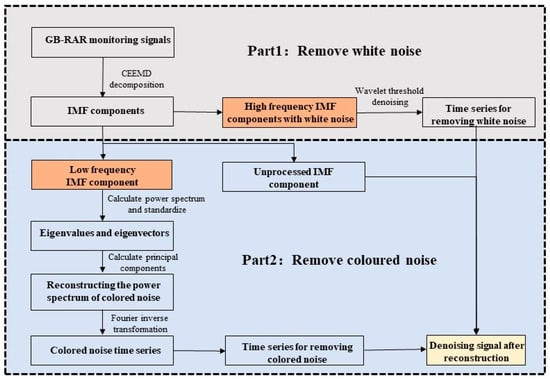
Figure 1.
Flowchart for denoising GB-RAR bridge pier monitoring data.
2.5. Evaluation of Denoising Effect
Monitoring data denoising is the use of denoising methods to remove noise from the original monitoring data and obtain more authentic and reliable monitoring data. For the quantification of denoising effect, Root Mean Square Error (RMSE) and SNR are usually used for evaluation [44].
- (1)
- RMSE
The RMSE indicates the mean square of the sum of the squares of the differences between the original monitoring data and the denoised monitoring data; the smaller the value, the better the denoising effect, which is calculated by the formula:
where is the signal length, is the original signal, and is the denoised signal.
- (2)
- SNR
The SNR is the ratio of signal power to noise signal power. The larger the value, the more significant the proportion of valuable signals and the better the denoising effect. The calculation formula is as follows:
3. Engineering Examples
3.1. Objects of Monitoring
The object of monitoring is the East Lake High-tech Bridge, located in the East Lake High-tech Development Zone of Wuhan City. It spans the Wuhan-Guangzhou high-speed railway, crossing subway line 11 and the High-tech Avenue. The bridge structure is a supported beam high-speed railway bridge spanning 32.6 m. The total length of the bridge is 293.4 m, and ten piers support it. Piers 6, 7, and 8 are each underpinned by eight bored piles with a diameter of 1 m, with lengths of 18 m, 18.5 m, and 19 m, respectively.
3.2. Overview of the Monitoring Program and Measurements
The deformation state of East Lake High-tech Bridge’s piers under regular usage was continuously monitored using the IBIS-S (Image by Interferometric System-Structures) ground-based interferometric radar system, developed collaboratively by the Italian IDS Company (Pisa) and the University of Florence (Florence). During the observation period, the IBIS-S system was placed in a smooth position at the base of Pier 5, enabling the surveillance of three distinct piers. Figure 2 offers a schematic representation of the IBIS-S system as it monitors the bridge. The monitoring utilized a persistent, uninterrupted mode for high-precision surveillance of the East Lake High-tech Bridge, with a maximum observation distance set at 200 m and a high-frequency data acquisition mode of 20 Hz. In Figure 2, the white arrow denotes the positions of the three piers of the East Lake High-tech Bridge in order of proximity: Pier 6, Pier 7, and Pier 8. Figure 3 shows the GB-RAR monitoring data of three piers.
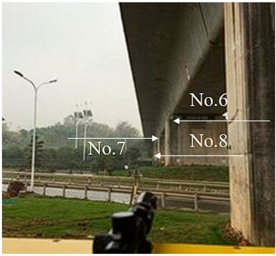
Figure 2.
View of the IBIS-S system monitoring bridges.
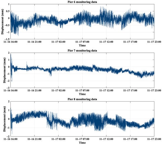
Figure 3.
Displacement time series of three piers.
Figure 3 shows the displacement time series of three bridge piers monitored by the IBIS-S system. It is evident from the graph that there are numerous spikes in the data from three piers, compromising the interpretation of the genuine deformation information. Within the monitoring timeframe, the deformation range for most of the three piers is predominantly within 1 mm. Pier 6 recorded a maximum deformation of 0.82 mm and a minimum deformation of −1.26 mm. For Pier 7, the maximum and minimum deformations were 1.81 mm and −2.11 mm, respectively. Pier 8 had a peak deformation of 1.27 mm and a trough of −1.73 mm. The deformation value of the displacement time series for Pier 7 reached its maximum within 40 min after monitoring commenced, exceeding 1 mm. After that, the deformation magnitude of Pier 7 stabilized, fluctuating within an approximate range of ±1 mm. Considering that the East Lake High-tech Bridge is a high-speed railway bridge, its deformation is influenced by the vibrations caused by passing high-speed trains. Furthermore, other environmental conditions and external factors can also have an impact on the monitoring data. Figure 4 shows the power spectrum density plots of the monitored data from the three piers. From the overall morphology, no distinct peaks or troughs stand out in the power spectrum of the three piers. Across both low and high frequencies, there is a slanting trend without any discontinuities. In the mid-to-low-frequency range, specifically from 10 to 5 Hz to 10−2 Hz, the power spectrum density escalates as the frequency decreases. By computing the spectral indices of the three power spectra, we determined that the indices for Piers 6, 7, and 8 were −0.96, −1.11, and −0.94, respectively. Thus, the bridge monitoring data were influenced by coloured and white noise. Consequently, upon acquiring pier monitoring data, it is imperative to mitigate the effects of noise, enhancing the accuracy of the data, which in turn will obtain the bridge’s authentic deformation data.
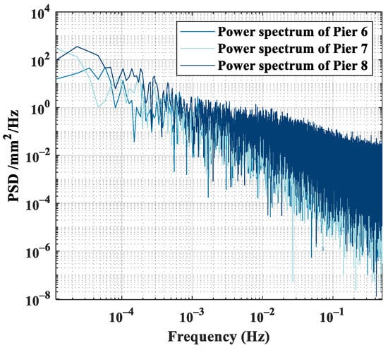
Figure 4.
Power spectrum of three piers monitoring data.
4. Experimental Results
4.1. A Denoising Method Based on CEEMD-WTD
After processing the monitoring data from the IBIS-S system of three bridge piers with CEEMD, the corresponding Intrinsic Mode Function (IMF) components are obtained. These IMF components represent the fundamental vibration patterns in the signal and can separate noise from the deformation data, thereby improving the signal-to-noise ratio of the data, as shown in the Figure 5, Figure 6 and Figure 7 below:
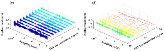
Figure 5.
(a) shows the IMF components from layer 1 to layer 10 obtained by CEEMD of the monitoring data from Pier 6. (b) shows the IMF components from layer 11 to layer 19 obtained by CEEMD of the monitoring data from Pier 6.
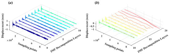
Figure 6.
(a) shows the IMF components from layer 1 to layer 10 obtained by CEEMD of the monitoring data from Pier 7. (b) shows the IMF components from layer 11 to layer 19 obtained by CEEMD of the monitoring data from Pier 7.
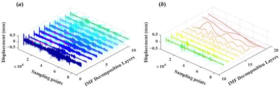
Figure 7.
(a) shows the IMF components from layer 1 to layer 10 obtained by CEEMD of the monitoring data from Pier 8. (b) shows the IMF components from layer 11 to layer 19 obtained by CEEMD of the monitoring data from Pier 8.
The decomposition of the monitoring data from the three piers using CEEMD yielded 19 IMF components in descending frequency order, with the final component representing the residual. Each IMF component represents an oscillation mode at different time scales within the signal, with frequencies arranged from high to low. The first few layers of the IMF are high-frequency IMF components, which typically correspond to high-frequency vibrations or noise in the bridge pier structure, including transient impacts from vehicles passing by and minute vibrations caused by wind loads, etc. The latter layers of the IMF are low-frequency IMF components, which usually correspond to low-frequency vibrations in the bridge pier structure caused by factors such as temperature changes, foundation settlements, and long-term load effects. These components reflect the overall deformation trends or long-term stability issues of the structure. The last layer of the IMF component is the residual term, which represents the long-term deformation, ageing, or cumulative effects of environmental factors on the bridge pier. Given the properties of CEEMD, summing all decomposed IMF components will reproduce the original monitoring data. As can be observed from Figure 5, Figure 6 and Figure 7, the first IMF component of the three piers is notably affected by white noise, with its deformation values significantly exceeding those of the subsequent IMF components. As the number of IMF decompositions increases, the deformation trend of the subsequent IMF components stabilizes. Therefore, it is essential to identify the boundary between the IMF components containing noise and those carrying the data, then process the determined white noise IMF components through the WTD method to remove the white noise.
In this study, we computed the energy entropy values of each IMF component to identify the boundary between noise and signal components. Following CEEMD of the monitoring data, we calculated the energy entropy value for each IMF component sequentially. The energy entropy values’ local minimum served as the demarcation between noise and signal IMF components. IMF components preceding this local minimum in energy entropy were classified as noise and subjected to WTD.
Figure 8 shows the line graph of the energy entropy values of each IMF component for the monitoring data of the three piers. For all three piers, the first local minimum of the energy entropy value corresponds to the second layer IMF component. For Pier 6, the second local minimum is at the seventh component IMF; for Pier 7, it is at the fifth layer IMF; and for Pier 8, it is at the fourth component IMF. Characteristics derived from the decomposition of monitoring data using the CEEMD method indicate that the initial high-frequency IMF component contains a higher proportion of noise. Their deformation values significantly exceed those of the subsequent low-frequency IMF component, thus classifying them as noise-related IMF components. Figure 6 demonstrates that the energy entropy minima for all three piers’ decomposed IMF components point to the second IMF component, suggesting the first IMF component is predominantly noise. However, merely processing the first IMF component does not entirely address the white noise present in the high-frequency IMF. The subsequent high-frequency IMF components may still contain white noise. Therefore, when the first minimum energy entropy value appears in the second IMF component, it becomes necessary to identify the second minimum energy entropy value as the demarcation between noise and signal IMF components. Accordingly, IMF components preceding this second minimum should be subjected to wavelet threshold denoising to remove white noise effectively.
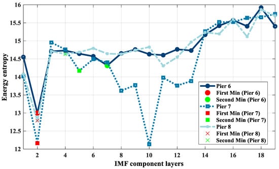
Figure 8.
Energy entropy values for each of the 19 layers of IMF components obtained from CEEMD of the monitoring data for the three piers.
In the process of using WTD to treat the monitoring data, different wavelet base functions and decomposition layers can affect the denoising results. This paper employs the soft threshold function and the Herature threshold algorithm using SNR and RMSE as evaluation criteria to comprehensively analyze the denoising effects of different wavelet base functions and decomposition layers. Firstly, we employed three commonly used wavelet families, Daubechies, Symlets, and Coiflets, to denoise the selected high-frequency noise IMF components. Table 1 compares the denoising effects of three wavelet systems. With the increase in the index of the wavelet basis function, the signal-to-noise ratio (SNR) first increases and then reaches a plateau. Among them, the SNR of the monitored data after processing with the sym9 wavelet is 8.3, which is the highest SNR value among the three wavelet systems after denoising. This indicates that sym9 has the best applicability in denoising GB-RAR monitoring data, as it can effectively remove noise while preserving the original features of the signal. Therefore, we select sym9 as the optimal wavelet basis function for this dataset. Furthermore, the denoising effect of the monitoring data with the sym9 wavelet function at different decomposition layers is as shown in Table 2.

Table 1.
Comparison of the denoising effect of three wavelet system decompositions with four layers.
Table 2.
Denoising effect of sym9 wavelet with different numbers of decomposition layers.
Direct WTD of the GB-RAR bridge monitoring data using the sym9 wavelet with different decomposition layers produces the results shown in Table 2. From Equations (22) and (23), it can be seen that the RMSE value is directly proportional to the () value in its definition, and as this part serves as the denominator in the SNR, it is inversely proportional to the SNR. As observed in Table 2, with the increase in the number of decomposition layers, the SNR of the monitoring data gradually decreases, and the RMSE gradually increases. This indicates that a lower number of decomposition layers will better preserve the original characteristics of the signal, but will also retain more noise from the original signal. In the wavelet threshold decomposition process, choosing a larger number of decomposition layers will remove the true signal components from the GB-RAR monitoring signal. Figure 9 and Figure 10 show the denoising effect on Pier 6 using 4-layer and 5-layer Sym9 wavelet decomposition, respectively. Comparing Figure 9 and Figure 10, it can be seen that the amount of information in the denoised signal when the decomposition layer is five is less than that when the decomposition layer is four, meaning that the best effect of WTD is achieved when the wavelet decomposition layer is 4. In summary, it can be concluded that the appropriate number of wavelet decomposition layers for processing the bridge monitoring data in this case is four.
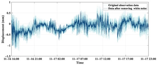
Figure 9.
The denoising results of Sym9 wavelet decomposition using a 4-layer decomposition for Pier 6.
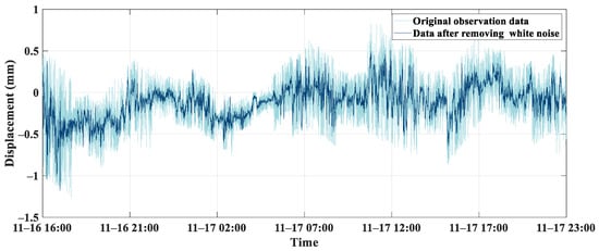
Figure 10.
The denoising results of Sym9 wavelet decomposition using a 5-layer decomposition for Pier 6.
After the above analysis, the Sym9 wavelet function and a decomposition level of four were determined to be appropriate for processing the current GB-RAR monitoring data. Each pier’s high-frequency IMF noise terms were denoised using WTD. The results are presented in the following Figure 11:
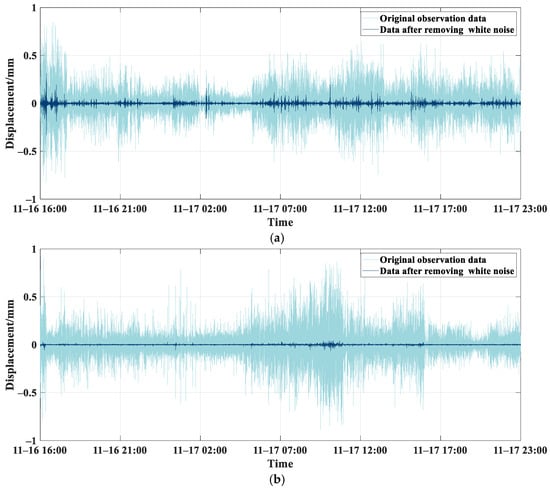
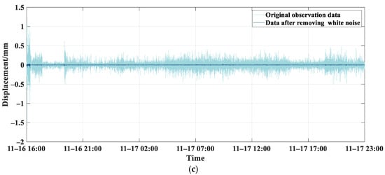
Figure 11.
CEEMD-WTD combination denoising results. (a) High frequency IMF components denoising results for Pier 6. (b) High frequency IMF components denoising results for Pier 7. (c) High frequency IMF components denoising results for Pier 8. (a) shows the WTD results of the high-frequency IMF component obtained by summing the IMF components from layer 1 to layer 6 of Pier 6 after CEEMD using Sym9 wavelet decomposition with 4 layers. (b) shows the WTD results of the high-frequency IMF component obtained by summing the IMF components from layer 1 to layer 4 of Pier 7 after CEEMD using Sym9 wavelet decomposition with 4 layers. (c) shows the WTD results of the high-frequency IMF component obtained by summing the IMF components from layer 1 to layer 3 of Pier 8 after CEEMD using Sym9 wavelet decomposition with 4 layers).
Traditional CEEMD denoising involves directly removing the selected high-frequency IMF component to achieve noise reduction. However, this approach may eliminate the signal details within the high-frequency IMF components, leading to distortion. Using wavelet threshold denoising on these high-frequency IMF components ensures the maximum retention of characteristic information within the high-frequency data. As shown in Figure 11, after WTD, the noise in the high-frequency IMF was eliminated while preserving a limited amount of characteristic information. We evaluated the post-denoising effect of CEEMD-WTD using two metrics: SNR and RMSE.
According to Table 3, the combined CEEMD-WTD approach improved over the standalone WTD method regarding SNR results. Specifically, the SNR for the three piers increased from 8.3 to 8.61, 16.67 to 19.87, and 11.17 to 15.06, respectively. Meanwhile, the RMSE of Pier 7 and Pier 8 are decreased by 0.02 mm and 0.06 mm. In summary, the CEEMD-WTD method performs better in eliminating white noise.
Table 3.
Comparison of SNR and RMSE among the three denoised methods.
4.2. Coloured Noise Removal Using PCA
The presence of coloured noise in the low-frequency power spectrum of the GB-RAR pier monitoring data indicates that coloured noise is typically allocated to principal components with smaller contribution degrees. By using the PCA algorithm and ignoring these principal components, a certain level of denoising can be achieved. Therefore, it is necessary to process the power spectrum of the low-frequency IMF vectors after CEEMD. We distinguish between low and high-frequency IMF vectors by counting the number of times each IMF component crosses zero. High-frequency IMF, with its intense fluctuations, crosses zero more frequently, while low-frequency IMF does so less often due to fewer fluctuations. Figure 12 shows the zero-crossing times for each IMF component of the three piers:
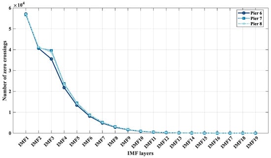
Figure 12.
Number of times each IMF component crosses zero for 19 layers of the IMF at three piers.
Based on Figure 12, as the number of decomposed IMF components increases, the zero-crossing occurrences of each IMF component diminish, aligning with the concept that the IMF frequencies decayed from CEEMD are arranged from high to low frequencies. Due to the decomposition of monitoring data from all three bridge piers into 19 layers of IMFs, this paper refers to the intuitive display of the severity of IMF layers for the bridge pier decomposed by CEEMD in Figure 7. Additionally, based on the quantitative representation in Figure 12, it is visually observed that starting from the 8th IMF layer, the vibration amplitude is smoother compared to the first seven IMF layers. Furthermore, there is a significant reduction in the number of zero-crossings of the IMF. This indicates that the IMFs beyond the eighth layer contain less white noise. In order to find the demarcation point between high-frequency IMFs and low-frequency IMFs, it is preliminarily considered that this point is around IMF8 and IMF9. Taking Pier No. 6 as an example, this paper calculates the slopes of the zero-crossing frequency curves of three sets of undetermined IMFs for this pier and selects the most appropriate demarcation point.
As shown in Table 4 above, by comparing the absolute values of the slopes of the zero-crossing frequency curves of IMF, it is found that the rate of decrease in the curve from IMF7 to IMF8 is more severe than that from IMF8 to IMF9. The number of zero crossings for the 19 IMF components of the three piers stabilizes after the eighth IMF component. Thus, this study designates the eighth IMF component as the boundary between high and low-frequency IMF for the GB-RAR monitoring data of the three bridge piers. Consequently, IMFs from layers 1 to 7 were classified as high-frequency components, while those from layers 8 to 19 were considered low-frequency. The low-frequency monitoring data, comprising IMFs from layers 8 to 19, was denoised using PCA. Initially, each pier’s low-frequency IMF trend component was removed from the monitoring data. Subsequently, the periodogram method was used to compute the power spectrum of each pier’s monitoring data. The power spectrum from the three piers was then aggregated into a matrix, which was subject to PCA to ascertain the contribution rate of each principal component. The computed principal components encompass the feature information of the three bridge piers. From Table 5, the contribution rate of each principal component varies and shows a decreasing trend. Table 5 indicates that the first and second principal components, after PCA of the power spectrum matrix, account for 89.3% of the feature information of the three piers. During monitoring, environmental factors, instrument system errors, or external interferences may introduce coloured noise, exhibiting time-correlated or periodic changes. Given that coloured noise primarily influences the monitoring data, the power spectrum derived from the first and second principal components will inherently include the characteristics of this coloured noise.
Table 4.
IMF zero-crossing frequency curve slope.
Table 5.
Contributions of the principal components of the low-frequency power spectrum.
In Section 2.4, Step 5, the power spectrum containing coloured noise in the first and second principal components was converted from the frequency domain to the time domain through inverse Fourier transformation. This obtained a displacement time series representing the coloured noise in the GB-RAR monitoring data. By subtracting this coloured noise displacement time series from the original monitoring displacement time series, we obtained the bridge pier monitoring data of the low-frequency IMF component without coloured noise. The final denoised monitoring data were reconstructed by combining the PCA denoised low-frequency IMF, WTD high-frequency components, and the original untreated IMF components. The low-frequency IMF component’s post-coloured noise removal was illustrated in Figure 13.
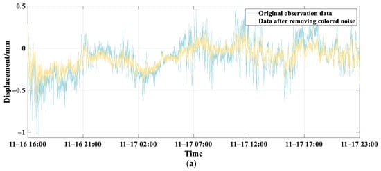
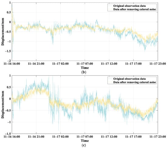
Figure 13.
Low-frequency IMF components of three bridge piers after removing coloured noise through PCA. (a) Low-frequency IMF component of Pier 6 after removing coloured noise through PCA. (b) Low-frequency IMF component of Pier 7 after removing coloured noise through PCA. (c) Low-frequency IMF component of Pier 8 after removing coloured noise through PCA.
Figure 13 shows that after removing the coloured noise, the three low-frequency IMF subcomponents retained their original deformation trends. The sudden spike deformations decreased in the data for all three piers, and the overall deformation trend became smoother. This is attributed to the dominant role of the non-stationary coloured noise in the original monitoring data. The data for Pier 7 from 17:00 to 23:00 on November 17th shows a reduction in the overall offset towards gravity direction. The monitoring data for Pier 8 showed a decrease in deformation values from 19:00 on November 16th to 12:00 on November 17th, with the deformation range narrowing to less than 0.5 mm.
Figure 14 shows that the original monitoring data exhibited significant deformation fluctuations before noise removal. After employing the combined denoising technique, the deformation amplitude of the GB-RAR monitoring data for the three bridge piers diminished. Notably, the peaks in deformation were reduced, and the overall deformation trend became more stable. Furthermore, the denoised data effectively retained the original monitoring data’s local deformation features while minimizing noise interference. This accurate identification of pier deformation ensures that the deformation monitoring data more closely reflects the actual state. Comparing the results from the combined denoising method with those from the standalone WTD approach, one can discern from the denoised data of Pier 6 in Figure 14 and Figure 9’s Pier 6 WTD denoised data that the combined method not only reduces sharp peak variations but also maximally preserves the deformation trend. It effectively tackles both the stationary white noise and the non-stationary coloured noise. Finally, the efficacy of the denoising is evaluated by calculating the uncertainty of the monitoring data, with results presented in Table 6.
Figure 14.
Monitoring data after denoising of three bridge piers. (a) Monitoring data after denoising of Pier 6. (b) Monitoring data after denoising of Pier 7. (c) Monitoring data after denoising of Pier 8.
Table 6.
Uncertainty of monitoring data before and after noise removal.
Upon comparing the uncertainty of the data post-denoising, it is evident that the uncertainty for each bridge pier decreased following the combined denoising process. The sample uncertainties for the three bridge piers were reduced by 43.2%, 35.8%, and 33.1%, respectively. This suggests that the post-denoise monitoring data more closely aligns with the actual deformation values, thus enhancing the accuracy of the monitoring data. The experimental results underscore that the combined CEEMD-WTD and PCA approach is a practical and pragmatic method for eliminating coloured and Gaussian white noise.
4.3. Comparative Experiment of CEEMD-WTD and PCA Denoising Methods
To demonstrate the superiority and reliability of the algorithm, this paper experimentally compares the combined CEEMD-WTD and PCA denoising method with the Kalman filter, Gaussian filter, moving average filter, and robust empirical mode decomposition (REMD) based on the uncertainty reduction rate before and after denoising. REMD, published in 2022 [45], is an improved empirical mode decomposition method based on the Soft Screening Stop Criterion (SSSC). The first three methods were chosen for comparison experiments mainly because they are commonly used denoising methods for deformation monitoring with mature technology and reliable results obtained, and REMD was chosen mainly because of its advancement. SSSC is an adaptive screening stopping criterion for automatically stopping the screening process of EMD. It automatically stops the screening process of EMD by extracting a set of single-component signals from the mixed signals, which reduces modal aliasing and improves the stability of the decomposition. It can cope with some problems that EMD cannot cope with, such as data that are too noisy or data with irregular outliers. Therefore, using REMD as a control experiment helps to objectively evaluate the validity of the method in this study. A comparison of the uncertainty reduction rates before and after denoising using these four methods is given in Table 7, where only the comparative plots for the Pier 8 filtering treatment, where the changes are relatively stable, are selected for display, as shown in Figure 15.
Table 7.
Comparison of the uncertainty reduction rate of each denoising algorithm.
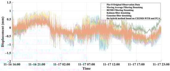
Figure 15.
Comparison of the filter processing of Pier 8.
By comparing the experimental results, it can be known that the uncertainty reduction rate of the CEEMD-WTD combined PCA denoising method is higher than that of the four denoising filters selected in this experiment because the proposed algorithm can decompose the signal into multiple scales of IMF. This allows it to pick up subtle changes in the signal that other traditional filtering methods cannot do, and this multi-scale decomposition capability gives CEEMD-WTD an advantage when dealing with complex monitoring data. In addition, compared with other methods, the CEEMD-WTD algorithm innovatively enhances its adaptability to various types of noise by introducing white noise, thus achieving lower error and higher uncertainty reduction rate in monitoring data.
It can be considered that the filtering algorithm of CEEMD-WTD combined PCA significantly reduces the uncertainty of state estimation. At the same time, the algorithm can extract useful signals accurately and reduce the influence of noise greatly, which also implies that the denoising effect of the improved filter is more stable.
5. Conclusions
Addressing the noise issues in GB-RAR bridge monitoring, we proposed a hybrid method based on CEEMD-WTD and PCA to eliminate both white and coloured noises, enhancing the precision of GB-RAR bridge monitoring data. Post CEEMD of the monitoring data, the high-frequency noise IMF components and the power spectrum of the low-frequency IMF component were treated with WTD and PCA, respectively. This facilitated the extraction of accurate bridge deformation information. The experimental results yield the following conclusions:
- (1)
- The CEEMD-WTD method, compared to WTD, is more proficient at extracting bridge deformation data against a background of white noise. After de-noising, the SNR for the three bridge piers were 8.61 dB, 19.87 dB, and 15.06 dB, respectively, with RMSE of 0.1 mm, 0.06 mm, and 0.09 mm. By harnessing the strengths of both denoising methods, this approach improves the SNR while retaining deformation characteristics, making it apt for bridge monitoring data denoising.
- (2)
- Using the low-frequency IMF component from three concurrently monitored adjacent bridge piers as input data and processing the CEEMD-decomposed power spectrum matrix composed of these components through PCA, we effectively removed the principal components of the coloured noise spectrum. This mitigated the effects of coloured noise and attenuated abrupt local deformation trends, showcasing its efficacy as a denoising method.
- (3)
- Upon employing the combined CEEMD-WTD and PCA method to remove white and coloured noises, the uncertainties for the three piers were 0.129, 0.212, and 0.303, respectively. These were reduced by 43.2%, 35.8%, and 33.1%. The reduction rates are high compared to other denoising methods, indicating that the combined denoising method reduces the effect of noise while retaining the real bridge deformation data.
Author Contributions
Conceptualization, Y.Y. and A.S.; Methodology, L.Z.; Software, P.L., Y.Y. and A.S.; Validation, Y.Y.; Formal analysis, W.Z.; Investigation, W.Z.; Resources, X.L. and J.M.; Data curation, P.L. and A.S.; Writing—original draft, L.Z.; Writing—review & editing, L.Z.; Visualization, P.L.; Supervision, X.L. and J.M.; Project administration, W.Z.; Funding acquisition, L.Z. and X.L. All authors have read and agreed to the published version of the manuscript.
Funding
This work was supported by the National Natural Science Foundation of China (Grant Nos. 42264004 and 42474026), the National Key Research and Development Program of China (Grant No. 2021YFB2600400), the Guangxi Key Technologies R&D Program (Grant No. GUIKE AB24010144), the Central Guidance for Local Scientific and Technological Development Funding Project (Grant No. GUIKE ZY24212008), the Open Fund of Technology Innovation Center for Geohazard Monitoring and Risk Early Warning, Ministry of Natural Resources (Grant No. TICGM-2024-07), the Open Fund of Hubei Luojia Laboratory (Grant No. 230100018).
Data Availability Statement
The original contributions presented in this study are included in the article.
Conflicts of Interest
Author Jun Ma was employed by China Railway Siyuan Survey and Design Group Co., Ltd. The remaining authors declare that the research was conducted in the absence of any commercial or financial relationships that could be construed as a potential conflict of interest. The funders had no role in the design of the study; in the collection, analyses, or interpretation of data; in the writing of the manuscript; or in the decision to publish the results.
References
- Stiros, S.; Psimoulis, P.; Moschas, F.; Saltogianni, V.; Tsantopoulos, E.; Triantafyllidis, P. Multi-sensor measurement of dynamic deflections and structural health monitoring of flexible and stiff bridges. Bridge Struct. 2019, 15, 43–51. [Google Scholar] [CrossRef]
- Xi, R.; He, Q.; Meng, X. Bridge monitoring using multi-GNSS observations with high cutoff elevations: A case study. Measurement 2021, 168, 108303. [Google Scholar] [CrossRef]
- Niu, Y.; Ye, Y.; Zhao, W.; Shu, J. Dynamic monitoring and data analysis of a long-span arch bridge based on high-rate GNSS-RTK measurement combining CF-CEEMD method. J. Civ. Struct. Health Monit. 2021, 11, 35–48. [Google Scholar] [CrossRef]
- Vicente, M.A.; Gonzalez, D.C.; Minguez, J.; Schumacher, T. A novel laser and video-based displacement transducer to monitor bridge deflections. Sensors 2018, 18, 970. [Google Scholar] [CrossRef] [PubMed]
- Farneti, E.; Cavalagli, N.; Costantini, M.; Trillo, F.; Minati, F.; Venanzi, I.; Ubertini, F. A method for structural monitoring of multispan bridges using satellite InSAR data with uncertainty quantification and its pre-collapse application to the Albiano-Magra Bridge in Italy. Struct. Health Monit. 2023, 22, 353–371. [Google Scholar] [CrossRef]
- Long, S.; Liu, W.; Ma, J.; Tong, A.; Wu, W.; Zhu, C. Health monitoring and safety evaluation of bridge dynamic load with a ground-based real aperture radar. Surv. Rev. 2022, 54, 172–186. [Google Scholar] [CrossRef]
- Pieraccini, M.; Miccinesi, L.; Abdorazzagh Nejad, A.; Naderi Nejad Fard, A. Experimental dynamic impact factor assessment of railway bridges through a radar interferometer. Remote Sens. 2019, 11, 2207. [Google Scholar] [CrossRef]
- Zhou, L.; Guo, J.; Wen, X.; Ma, J.; Yang, F.; Wang, C.; Zhang, D. Monitoring and analysis of dynamic characteristics of super high-rise buildings using GB-RAR: A case study of the WGC under construction, China. Appl. Sci. 2020, 10, 808. [Google Scholar] [CrossRef]
- Zhang, Z.; Suo, Z.; Tian, F.; Qi, L.; Tao, H.; Li, Z. A novel GB-SAR system based on TD-MIMO for high-precision bridge vibration monitoring. Remote Sens. 2022, 14, 6383. [Google Scholar] [CrossRef]
- Liu, X.; Zhao, S.; Wang, P.; Wang, R.; Huang, M. Improved data-driven stochastic subspace identification with autocorrelation matrix modal order estimation for bridge modal parameter extraction using GB-SAR Data. Buildings 2022, 12, 253. [Google Scholar] [CrossRef]
- Hu, J.; Guo, J.; Zhou, L.; Zhang, S.; Chen, M.; Hang, C. Dynamic vibration characteristics monitoring of high-rise buildings by interferometric real-aperture radar technique: Laboratory and full-scale tests. IEEE Sens. J. 2018, 18, 6423–6431. [Google Scholar] [CrossRef]
- Kuras, P.; Ortyl, Ł.; Owerko, T.; Salamak, M.; Łaziński, P. GB-SAR in the diagnosis of critical city infrastructure—A case study of a load test on the long tram extradosed bridge. Remote Sens. 2020, 12, 3361. [Google Scholar] [CrossRef]
- Gao, Z.; Di, H.; Zhuo, Y.; Jia, Y.; Liu, S.; Zhang, X. Rating for operational performance of high-speed railway bridges based on Ground-based Interferometry Radar. J. China Railw. Soc. 2023, 45, 153–160. [Google Scholar]
- Wang, C.; Zhou, L.; Ma, J.; Shi, A.; Li, X.; Liu, L.; Zhang, Z.; Zhang, D. GB-RAR Deformation Information Estimation of High-Speed Railway Bridge in Consideration of the Effects of Colored Noise. Appl. Sci. 2022, 12, 10504. [Google Scholar] [CrossRef]
- Hu, J.; Guo, J.; Xu, Y.; Zhou, L.; Zhang, S.; Fan, K. Differential ground-based radar interferometry for slope and civil structures monitoring: Two case studies of landslide and bridge. Remote Sens. 2019, 11, 2887. [Google Scholar] [CrossRef]
- Xiong, Q.; Xiong, H.; Yuan, C.; Kong, Q. A novel deep convolutional image-denoiser network for structural vibration signal denoising. Eng. Appl. Artif. Intell. 2023, 117, 105507. [Google Scholar] [CrossRef]
- Ke, L. Denoising GPS-Based Structure Monitoring Data Using Hybrid EMD and Wavelet Packet. Math. Probl. Eng. 2017, 2017, 4920809. [Google Scholar] [CrossRef]
- Zhang, D.; Wang, S.; Li, F.; Wang, J.; Sangaiah, A.K.; Sheng, V.S.; Ding, X. An ECG signal de-noising approach based on wavelet energy and sub-band smoothing filter. Appl. Sci. 2019, 9, 4968. [Google Scholar] [CrossRef]
- Chen, X.; Zhao, X.; Liang, Y.; Luan, X. Denoising Ocean Turbulence Microstructure Signals for Application in Estimating Turbulence Kinetic Energy Dissipation Rates Based on EMD-PCA. Sensors 2022, 22, 4413. [Google Scholar] [CrossRef]
- Huang, N.E.; Shen, Z.; Long, S.R.; Wu, M.C.; Shih, H.H.; Zheng, Q.; Yen, N.-C.; Tung, C.C.; Liu, H.H. The empirical mode decomposition and the Hilbert spectrum for nonlinear and non-stationary time series analysis. Proc. R. Soc. London Ser. A Math. Phys. Eng. Sci. 1998, 454, 903–995. [Google Scholar] [CrossRef]
- Chen, W.; Li, J.; Wang, Q.; Han, K. Fault feature extraction and diagnosis of rolling bearings based on wavelet thresholding denoising with CEEMDAN energy entropy and PSO-LSSVM. Measurement 2021, 172, 108901. [Google Scholar] [CrossRef]
- Yeh, J.-R.; Shieh, J.-S.; Huang, N.E. Complementary ensemble empirical mode decomposition: A novel noise enhanced data analysis method. Adv. Adapt. Data Anal. 2010, 2, 135–156. [Google Scholar] [CrossRef]
- Gaci, S. A new ensemble empirical mode decomposition (EEMD) denoising method for seismic signals. Energy Procedia 2016, 97, 84–91. [Google Scholar] [CrossRef]
- Cheng, X.; Mao, J.; Li, J.; Zhao, H.; Zhou, C.; Gong, X.; Rao, Z. An EEMD-SVD-LWT algorithm for denoising a lidar signal. Measurement 2021, 168, 108405. [Google Scholar] [CrossRef]
- Peng, K.; Guo, H.; Shang, X. EEMD and multiscale PCA-based signal denoising method and its application to seismic P-phase arrival picking. Sensors 2021, 21, 5271. [Google Scholar] [CrossRef]
- Huimin, C.; Ruimei, Z.; Yanli, H. Improved threshold denoising method based on wavelet transform. Phys. Procedia 2012, 33, 1354–1359. [Google Scholar] [CrossRef]
- Jiang, X.; Lang, Q.; Jing, Q.; Wang, H.; Chen, J.; Ai, Q. An improved wavelet threshold denoising method for health monitoring data: A case study of the Hong Kong-Zhuhai-Macao Bridge immersed tunnel. Appl. Sci. 2022, 12, 6743. [Google Scholar] [CrossRef]
- REN, A.; XU, K. Time domain signal extraction from GNSS time series with colored noise. Chin. J. Geophys. 2023, 66, 518–529. [Google Scholar]
- Abdullah, H.A.; Hanif, M.U.; Hassan, M.U.; Shahid, J.M.; Khan, S.A.; Ali, A. Improved damage assessment of bridges using advanced signal processing techniques of CEEMDAN-EWT and Kernal PCA. Eng. Struct. 2025, 329, 119774. [Google Scholar] [CrossRef]
- Liu, X.; Zhao, S.; Wang, R. ESMD-WSST high-frequency de-noising method for bridge dynamic deflection using GB-SAR. Electronics 2022, 12, 54. [Google Scholar] [CrossRef]
- Ma, J. BDS/GPS deformation analysis of a long-span cable-stayed bridge based on colored noise filtering. Geod. Geodyn. 2023, 14, 163–171. [Google Scholar] [CrossRef]
- Langbein, J. Noise in GPS displacement measurements from Southern California and Southern Nevada. J. Geophys. Res. Solid Earth 2008, 113. [Google Scholar] [CrossRef]
- Li, Y.; Chen, C.; Fang, R.; Yi, L. Accuracy enhancement of high-rate GNSS positions using a complete ensemble empirical mode decomposition-based multiscale multiway PCA. J. Asian Earth Sci. 2019, 169, 67–78. [Google Scholar] [CrossRef]
- Wang, M.; Shang, J. Denoising method of steel frame structure settlement data based on CEEMD and improved Wavelet Threshold method. J. Geod. Geodyn. 2022, 42, 1191–1195. [Google Scholar]
- Xue, Y.; Cao, J. Seismic attenuation analysis using ensemble empirical mode decomposition and wavelet transform. Oil Geophys. Prospect. 2016, 51, 1148–1155. [Google Scholar]
- Wu, Z.; Huang, N.E. Ensemble empirical mode decomposition: A noise-assisted data analysis method. Adv. Adapt. Data Anal. 2009, 1, 1–41. [Google Scholar] [CrossRef]
- Li, J.; Liu, C.; Zeng, Z.; Chen, L. GPR signal denoising and target extraction with the CEEMD method. IEEE Geosci. Remote Sens. Lett. 2015, 12, 1615–1619. [Google Scholar]
- Wang, J.; He, X.; Ferreira, V.G. Ocean wave separation using CEEMD-Wavelet in GPS wave measurement. Sensors 2015, 15, 19416–19428. [Google Scholar] [CrossRef]
- Wang, S.; Zhao, X.; Liu, W.; Du, J.; Zhao, D.; Yu, Z. Impact-Type Sunflower Yield Sensor Signal Denoising Method Based on CEEMD-WTD. Agriculture 2023, 13, 166. [Google Scholar] [CrossRef]
- Jing-Yi, L.; Hong, L.; Dong, Y.; Yan-Sheng, Z. A new wavelet threshold function and denoising application. Math. Probl. Eng. 2016, 2016, 3195492. [Google Scholar] [CrossRef]
- Wang, X.; Huang, S.; Kang, C.; Li, G.; Li, C. Integration of wavelet denoising and HHT applied to the analysis of bridge dynamic characteristics. Appl. Sci. 2020, 10, 3605. [Google Scholar] [CrossRef]
- WANG, H.; YE, R.; Du, W. A hybrid denoising method for bridge vibration signal based on EMD and wavelet threshold. Highway 2021, 66, 110–116. [Google Scholar]
- Huang, L.; Fu, Y. Noise analysis of GPS continuous observation stations. J. Earthq. 2007, 29, 197–202. [Google Scholar]
- Zhang, R.; Zhang, P.; Zhao, F. CEEMDAN-SG based blast shock wave denoising algorithm research. Foreign Electron. Meas. Technol. 2022, 41, 119–125. [Google Scholar]
- Liu, Z.; Peng, D.; Zuo, M.J.; Xia, J.; Qin, Y. Improved Hilbert–Huang transform with soft sifting stopping criterion and its application to fault diagnosis of wheelset bearings. ISA Trans. 2022, 125, 426–444. [Google Scholar] [CrossRef]
Disclaimer/Publisher’s Note: The statements, opinions and data contained in all publications are solely those of the individual author(s) and contributor(s) and not of MDPI and/or the editor(s). MDPI and/or the editor(s) disclaim responsibility for any injury to people or property resulting from any ideas, methods, instructions or products referred to in the content. |
© 2025 by the authors. Licensee MDPI, Basel, Switzerland. This article is an open access article distributed under the terms and conditions of the Creative Commons Attribution (CC BY) license (https://creativecommons.org/licenses/by/4.0/).