Two High-Accuracy Linear Finite Difference Schemes for Rosenau–KdV–RLW Equation

Abstract

Two numerical methods are investigated for the initial–boundary value problem of a nonlinear Rosenau–KdV–RLW equation with homogeneous boundary conditions. With the premise of achieving second-order theoretical accuracy in the temporal direction, two-level linearization discretization and three-level extrapolated linearization discretization are applied to nonlinear terms, respectively. To achieve a higher theoretical accuracy in the spatial direction, the Richardson extrapolation combination technique is employed; thereby, a two-level linearized difference scheme and a three-level linear difference scheme for the Rosenau–KdV–RLW equation are proposed, both with a theoretical accuracy of $O({\tau }^2+h^4)$. The two-level difference scheme also reasonably simulates the conservation property of the problem. The convergence and stability of the two schemes are proven using mathematical induction and discrete functional analysis methods. The numerical results demonstrate the effectiveness of both schemes.

1. Introduction

Nonlinear waves in nature are a vital research area of scientific inquiry, with many scholars dedicated to developing mathematical models to explain these phenomena. Korteweg and de Vries established a partial differential equation for shallow water waves that propagate unidirectionally when studying small-amplitude, long waves in shallow water, known as the Korteweg–de Vries (KdV) equation [1]

$$\begin{array}{c}\hfill u_t+u_x+u{u}_x-u_{xxx}=0\end{array}$$

(1)

which has plenty of applications in numerous fields of physics, such as magnetohydrodynamic waves in plasma and ion-sound waves. When investigating long-wave motions in shallow water, Peregrine [2] introduced the regularized long-wave (RLW) equation

$$\begin{array}{c}\hfill u_t+u_x+u{u}_x-u_{xxt}=0\end{array}$$

(2)

which can explain different scenarios involving nonlinear dispersive waves from another perspective and attracted more attention due to its ability to accurately simulate most applications of the KdV Equation (1). In further research, scholars discovered that the KdV equation cannot describe wave–wave and wave–wall interactions. To overcome this shortcoming, the Rosenau equation [3,4] was proposed

$$\begin{array}{c}\hfill u_t+u_{xxxxt}+u_x+u{u}_x=0\end{array}$$

(3)

and many numerical methods have been discussed [5,6,7]. To explore more complex nonlinear wave phenomena, the Rosenau–KdV–RLW equation [8,9] can be derived by adding the viscous terms $-u_{xxt}$ and $u_{xxx}$ to the Rosenau Equation (3):

$$\begin{array}{c}\hfill u_t-u_{xxt}+u_{xxxxt}+u_x+u_{xxx}+u{u}_x=0.\end{array}$$

(4)

The Rosenau–KdV–RLW Equation (4) provides a more reasonable description of the dynamic characteristics of dispersive shallow water waves. Razborova et al. [10,11] gave the constraint conditions for the existence of soliton solutions to the Rosenau–KdV–RLW Equation (4) through the Ansatz method and obtained exact soliton solutions. Furthermore, the conservation laws for the Rosenau–KdV–RLW equation have been analyzed using the Lie symmetry analysis method [12].

Numerous studies have investigated numerical methods for the Rosenau–KdV–RLW Equation (4), including the finite element method [13], the B-spline differential quadrature method [14], the meshless radial basis function (RBF) collocation method [15], the Runge–Kutta method [16,17], and the finite difference method [18,19,20,21,22,23]. Among the finite difference approaches, the two-level nonlinear scheme [22] necessitates iterative nonlinear solvers, leading to high computational costs. In contrast, the three-level linear scheme [19] avoids nonlinear iterations but requires additional storage and lacks self-starting capabilities. To enhance the numerical accuracy, Ghiloufi [20] developed fourth-order spatially accurate schemes for the Rosenau–KdV–RLW equation using Richardson extrapolation. For two-dimensional cases, Labidi et al. [21] proposed a linearized conservative finite difference scheme that preserved the mass, admitted a unique solution, and was unconditionally stable.

In this paper, we consider the following initial and boundary value problem:

$$\begin{array}{c}{u}_t-u_{xxt}+u_{xxxxt}+u_x+u_{xxx}+u{u}_x=0,x\in (x_L,x_R),t\in (0,T],\hfill \end{array}$$

(5)

$$\begin{array}{c}u(x,0)=u_0\left(x\right),x\in [x_L,x_R],\hfill \end{array}$$

(6)

$$\begin{array}{c}u(x_L,t)=u(x_R,t)=0,u_{xx}(x_L,t)=u_{xx}(x_R,t)=0,t\in [0,T]\hfill \end{array}$$

(7)

where $u_0\left(x\right)$ is a known smooth function. Problem (5)–(7) has the conservative quantity [13,23]

$$\begin{array}{c}\hfill Q\left(t\right)={\int }_{x_L}^{x_R}u(x,t)dx={\int }_{x_L}^{x_R}{u}_0\left(x\right)dx=Q\left(0\right)\end{array}$$

(8)

in which $Q\left(0\right)$ is a constant only related to the initial conditions.

The outline of this paper is as follows. In Section 2, we present a two-level linearized finite difference scheme which includes the following components: (i) a detailed Richardson extrapolation derived via Taylor expansion in Section 2.1, (ii) a difference scheme with a theoretical accuracy of $O({\tau }^2+h^4)$ and an analysis of its conservation law in Section 2.2, and (iii) a theoretical analysis of the convergence and stability in Section 2.3. Subsequently, in Section 3.1, we construct a three-level linear difference scheme that achieves the same theoretical accuracy, along with a corresponding convergence and stability analysis. Finally, in Section 4, we conduct extensive numerical experiments, including waveform simulations of the numerical solutions, accuracy tests, and comparisons with existing results in the literature, to validate the proposed schemes.

2. The First Method: A Two-Level Linearized Finite Difference Scheme

2.1. Preliminaries

For the domain $[x_L,x_R]\times [0,T]$, let $h=(x_R-x_L)/J$ be the step size of the spatial grid and $\tau$ be the step size of the temporal direction such that $x_j=x_L+jh\left(0\le j\le J\right)$, $t_n=n\tau$ ($n=0,1,2,\cdots ,N$, $N=\left[T/\tau \right]$). Denote $u_j^n=u(x_j,t_n)$ as the exact value of $u(x,t)$ and $U_j^n\approx u(x_j,t_n)$ as the approximation of $u(x,t)$ at point $(x_j,t_n)$, respectively. Define

$$\begin{array}{ccc}& & {\left(U_j^n\right)}_x={\displaystyle \frac{U_{j+1}^n-U_j^n}{h}},{\left(U_j^n\right)}_{\overline{x}}={\displaystyle \frac{U_j^n-U_{j-1}^n}{h}},{\left(U_j^n\right)}_{\widehat{x}}={\displaystyle \frac{U_{j+1}^n-U_{j-1}^n}{2h}},\hfill \\ & & {\left(U_j^n\right)}_{\ddot{x}}={\displaystyle \frac{U_{j+2}^n-U_{j-2}^n}{4h}},{\left(U_j^n\right)}_t={\displaystyle \frac{U_j^{n+1}-U_j^n}{\tau }},U_j^{n+{\displaystyle \frac{1}{2}}}={\displaystyle \frac{U_j^{n+1}+U_j^n}{2}},\hfill \\ & & \langle U^n,V^n\rangle =h\sum _{j=1}^{J-1}{U}_j^n{V}_j^n,\parallel U^n{\parallel }^2=\langle U^n,U^n\rangle ,\parallel U^n{\parallel }_{\infty }=\underset{1\le j\le J-1}{max}\left|U_j^n\right|\hfill \end{array}$$

and

$$\begin{array}{ccc}& & Z_h^0=\{U=\left(U_j\right)|U_{-2}=U_{-1}=U_0=U_J=U_{J+1}=U_{J+2}=0,\hfill \\ & & j=-2,-1,0,\cdots ,J,J+1,J+2\}.\hfill \end{array}$$

According to Taylor expansion, if $u(x,t)$ is smooth enough, the following results hold:

$$\begin{array}{c}{\left(u_j^n\right)}_t={\left({\displaystyle \frac{\partial u}{\partial t}}\right)}_j^{n+{\displaystyle \frac{1}{2}}}+O\left({\tau }^2\right),\hfill \end{array}$$

(9)

$$\begin{array}{c}{\left(u_j^{n+{\displaystyle \frac{1}{2}}}\right)}_{\widehat{x}}={\left({\displaystyle \frac{\partial u}{\partial x}}\right)}_j^{n+{\displaystyle \frac{1}{2}}}+{\displaystyle \frac{1}{6}}{h}^2{\left({\displaystyle \frac{{\partial }^{3}u}{\partial x^3}}\right)}_j^{n+{\displaystyle \frac{1}{2}}}+O\left(h^4\right),\hfill \end{array}$$

(10)

$$\begin{array}{c}{\left(u_j^{n+{\displaystyle \frac{1}{2}}}\right)}_{\ddot{x}}={\left({\displaystyle \frac{\partial u}{\partial x}}\right)}_j^{n+{\displaystyle \frac{1}{2}}}+{\displaystyle \frac{2}{3}}{h}^2{\left({\displaystyle \frac{{\partial }^{3}u}{\partial x^3}}\right)}_j^{n+{\displaystyle \frac{1}{2}}}+O\left(h^4\right).\hfill \end{array}$$

(11)

Then, the combination of (10) and (11) yields

$$\begin{array}{c}{\displaystyle \frac{4}{3}}{\left(u_j^{n+{\displaystyle \frac{1}{2}}}\right)}_{\widehat{x}}-{\displaystyle \frac{1}{3}}{\left(u_j^{n+{\displaystyle \frac{1}{2}}}\right)}_{\ddot{x}}={\left({\displaystyle \frac{\partial u}{\partial x}}\right)}_j^{n+{\displaystyle \frac{1}{2}}}+O\left(h^4\right).\hfill \end{array}$$

(12)

Similarly, according to

$$\begin{array}{ccc}& & {\left(u_j^{n+{\displaystyle \frac{1}{2}}}\right)}_{x\overline{x}}={\left({\displaystyle \frac{{\partial }^{2}u}{\partial x^2}}\right)}_j^{n+{\displaystyle \frac{1}{2}}}+{\displaystyle \frac{1}{12}}{h}^2{\left({\displaystyle \frac{{\partial }^{4}u}{\partial x^4}}\right)}_j^{n+{\displaystyle \frac{1}{2}}}+O\left(h^4\right),\hfill \\ & & {\left(u_j^{n+{\displaystyle \frac{1}{2}}}\right)}_{\widehat{x}\widehat{x}}={\left({\displaystyle \frac{{\partial }^{2}u}{\partial x^2}}\right)}_j^{n+{\displaystyle \frac{1}{2}}}+{\displaystyle \frac{1}{3}}{h}^2{\left({\displaystyle \frac{{\partial }^{4}u}{\partial x^4}}\right)}_j^{n+{\displaystyle \frac{1}{2}}}+O\left(h^4\right),\hfill \\ & & {\left(u_j^{n+{\displaystyle \frac{1}{2}}}\right)}_{x\overline{x}\widehat{x}}={\left({\displaystyle \frac{{\partial }^{3}u}{\partial x^3}}\right)}_j^{n+{\displaystyle \frac{1}{2}}}+{\displaystyle \frac{1}{4}}{h}^2{\left({\displaystyle \frac{{\partial }^{5}u}{\partial x^5}}\right)}_j^{n+{\displaystyle \frac{1}{2}}}+O\left(h^4\right),\hfill \\ & & {\left(u_j^{n+{\displaystyle \frac{1}{2}}}\right)}_{x\overline{x}\ddot{x}}={\left({\displaystyle \frac{{\partial }^{3}u}{\partial x^3}}\right)}_j^{n+{\displaystyle \frac{1}{2}}}+{\displaystyle \frac{3}{4}}{h}^2{\left({\displaystyle \frac{{\partial }^{5}u}{\partial x^5}}\right)}_j^{n+{\displaystyle \frac{1}{2}}}+O\left(h^4\right),\hfill \\ & & {\left(u_j^{n+{\displaystyle \frac{1}{2}}}\right)}_{xx\overline{x}\overline{x}}={\left({\displaystyle \frac{{\partial }^{4}u}{\partial x^4}}\right)}_j^{n+{\displaystyle \frac{1}{2}}}+{\displaystyle \frac{1}{6}}{h}^2{\left({\displaystyle \frac{{\partial }^{6}u}{\partial x^6}}\right)}_j^{n+{\displaystyle \frac{1}{2}}}+O\left(h^4\right),\hfill \\ & & {\left(u_j^{n+{\displaystyle \frac{1}{2}}}\right)}_{x\overline{x}\widehat{x}\widehat{x}}={\left({\displaystyle \frac{{\partial }^{4}u}{\partial x^4}}\right)}_j^{n+{\displaystyle \frac{1}{2}}}+{\displaystyle \frac{5}{12}}{h}^2{\left({\displaystyle \frac{{\partial }^{6}u}{\partial x^6}}\right)}_j^{n+{\displaystyle \frac{1}{2}}}+O\left(h^4\right),\hfill \end{array}$$

we also have

$$\begin{array}{ccc}& & {\displaystyle \frac{4}{3}}{\left(u_j^{n+{\displaystyle \frac{1}{2}}}\right)}_{x\overline{x}}-{\displaystyle \frac{1}{3}}{\left(u_j^{n+{\displaystyle \frac{1}{2}}}\right)}_{\widehat{x}\widehat{x}}={\left({\displaystyle \frac{{\partial }^{2}u}{\partial x^2}}\right)}_j^{n+{\displaystyle \frac{1}{2}}}+O\left(h^4\right),\hfill \end{array}$$

(13)

$$\begin{array}{ccc}& & {\displaystyle \frac{3}{2}}{\left(u_j^{n+{\displaystyle \frac{1}{2}}}\right)}_{x\overline{x}\widehat{x}}-{\displaystyle \frac{1}{2}}{\left(u_j^{n+{\displaystyle \frac{1}{2}}}\right)}_{x\overline{x}\ddot{x}}={\left({\displaystyle \frac{{\partial }^{3}u}{\partial x^3}}\right)}_j^{n+{\displaystyle \frac{1}{2}}}+O\left(h^4\right),\hfill \end{array}$$

(14)

$$\begin{array}{ccc}& & {\displaystyle \frac{5}{3}}{\left(u_j^{n+{\displaystyle \frac{1}{2}}}\right)}_{xx\overline{x}\overline{x}}-{\displaystyle \frac{2}{3}}{\left(u_j^{n+{\displaystyle \frac{1}{2}}}\right)}_{x\overline{x}\widehat{x}\widehat{x}}={\left({\displaystyle \frac{{\partial }^{4}u}{\partial x^4}}\right)}_j^{n+{\displaystyle \frac{1}{2}}}+O\left(h^4\right)\hfill \end{array}$$

(15)

for $\tau ,h\to 0$.

Lemma 1.

If $u(x,t)$ is smooth enough, then

$$\begin{array}{ccc}& & {\displaystyle \frac{2}{3}}\left[u_j^n{\left(u_j^{n+1}\right)}_{\widehat{x}}+u_j^{n+1}{\left(u_j^n\right)}_{\widehat{x}}\right]-{\displaystyle \frac{1}{6}}\left[u_j^n{\left(u_j^{n+1}\right)}_{\ddot{x}}+u_j^{n+1}{\left(u_j^n\right)}_{\ddot{x}}\right]\hfill \\ & & ={\left(u{\displaystyle \frac{\partial u}{\partial x}}\right)}_j^{n+{\displaystyle \frac{1}{2}}}+O({\tau }^2+h^4)\hfill \end{array}$$

(16)

holds for $\tau ,h\to 0$.

Proof of Lemma 1.

Since

$$\begin{array}{c}{u}_j^n=u_j^{n+{\displaystyle \frac{1}{2}}}-{\displaystyle \frac{\tau }{2}}·{\left({\displaystyle \frac{\partial u}{\partial t}}\right)}_j^{n+{\displaystyle \frac{1}{2}}}+O\left({\tau }^2\right),\hfill \end{array}$$

(17)

$$\begin{array}{c}{u}_j^{n+1}=u_j^{n+{\displaystyle \frac{1}{2}}}+{\displaystyle \frac{\tau }{2}}·{\left({\displaystyle \frac{\partial u}{\partial t}}\right)}_j^{n+{\displaystyle \frac{1}{2}}}+O\left({\tau }^2\right),\hfill \end{array}$$

(18)

$$\begin{array}{c}{\displaystyle \frac{4}{3}}{\left(u_j^{n+1}\right)}_{\widehat{x}}-{\displaystyle \frac{1}{3}}{\left(u_j^{n+1}\right)}_{\ddot{x}}={\left({\displaystyle \frac{\partial u}{\partial x}}\right)}_j^{n+{\displaystyle \frac{1}{2}}}+{\displaystyle \frac{\tau }{2}}·{\left({\displaystyle \frac{{\partial }^{2}u}{\partial x\partial t}}\right)}_j^{n+{\displaystyle \frac{1}{2}}}+O({\tau }^2+h^4),\hfill \end{array}$$

(19)

$$\begin{array}{c}{\displaystyle \frac{4}{3}}{\left(u_j^n\right)}_{\widehat{x}}-{\displaystyle \frac{1}{3}}{\left(u_j^n\right)}_{\ddot{x}}={\left({\displaystyle \frac{\partial u}{\partial x}}\right)}_j^{n+{\displaystyle \frac{1}{2}}}-{\displaystyle \frac{\tau }{2}}·{\left({\displaystyle \frac{{\partial }^{2}u}{\partial x\partial t}}\right)}_j^{n+{\displaystyle \frac{1}{2}}}+O({\tau }^2+h^4)\hfill \end{array}$$

(20)

from (17)–(20), we have

$$\begin{array}{cc}& {\displaystyle \frac{2}{3}}\left[u_j^n{\left(u_j^{n+1}\right)}_{\widehat{x}}+u_j^{n+1}{\left(u_j^n\right)}_{\widehat{x}}\right]-{\displaystyle \frac{1}{6}}\left[u_j^n{\left(u_j^{n+1}\right)}_{\ddot{x}}+u_j^{n+1}{\left(u_j^n\right)}_{\ddot{x}}\right]\\ & ={\displaystyle \frac{1}{2}}\left\{u_j^n\left[{\displaystyle \frac{4}{3}}{\left(u_j^{n+1}\right)}_{\widehat{x}}-{\displaystyle \frac{1}{3}}{\left(u_j^{n+1}\right)}_{\ddot{x}}\right]+u_j^{n+1}\left[{\displaystyle \frac{4}{3}}{\left(u_j^n\right)}_{\widehat{x}}-{\displaystyle \frac{1}{3}}{\left(u_j^n\right)}_{\ddot{x}}\right]\right\}\\ & ={\displaystyle \frac{1}{2}}(u_j^{n+{\displaystyle \frac{1}{2}}}-A\tau )·\left[{\left({\displaystyle \frac{\partial u}{\partial x}}\right)}_j^{n+{\displaystyle \frac{1}{2}}}+B\tau \right]+{\displaystyle \frac{1}{2}}(u_j^{n+{\displaystyle \frac{1}{2}}}+A\tau )·\left[{\left({\displaystyle \frac{\partial u}{\partial x}}\right)}_j^{n+{\displaystyle \frac{1}{2}}}-B\tau \right]+O({\tau }^2+h^4)\\ & =u_j^{n+{\displaystyle \frac{1}{2}}}·{\left({\displaystyle \frac{\partial u}{\partial x}}\right)}_j^{n+{\displaystyle \frac{1}{2}}}-AB{\tau }^2+O({\tau }^2+h^4)\\ & ={\left(u{\displaystyle \frac{\partial u}{\partial x}}\right)}_j^{n+{\displaystyle \frac{1}{2}}}+O({\tau }^2+h^4)\end{array}$$

where $A={\displaystyle \frac{1}{2}}\left({\displaystyle \frac{\partial u}{\partial t}}\right){|}_j^{n+{\displaystyle \frac{1}{2}}}$, $B={\displaystyle \frac{1}{2}}\left({\displaystyle \frac{{\partial }^{2}u}{\partial x\partial t}}\right){|}_j^{n+{\displaystyle \frac{1}{2}}}$. This completes the proof. □

2.2. The Two-Level Numerical Scheme and the Conservative Law

Next, we propose a finite difference scheme for the problem (5)–(7) as follows:

$$\begin{array}{c}{\left(U_j^n\right)}_t-{\displaystyle \frac{4}{3}}{\left(U_j^n\right)}_{x\overline{x}t}+{\displaystyle \frac{1}{3}}{\left(U_j^n\right)}_{\widehat{x}\widehat{x}t}+{\displaystyle \frac{5}{3}}{\left(U_j^n\right)}_{xx\overline{x}\overline{x}t}-{\displaystyle \frac{2}{3}}{\left(U_j^n\right)}_{x\overline{x}\widehat{x}\widehat{x}t}\hfill \\ +{\displaystyle \frac{4}{3}}{\left(U_j^{n+{\displaystyle \frac{1}{2}}}\right)}_{\widehat{x}}-{\displaystyle \frac{1}{3}}{\left(U_j^{n+{\displaystyle \frac{1}{2}}}\right)}_{\ddot{x}}+{\displaystyle \frac{3}{2}}{\left(U_j^{n+{\displaystyle \frac{1}{2}}}\right)}_{x\overline{x}\widehat{x}}-{\displaystyle \frac{1}{2}}{\left(U_j^{n+{\displaystyle \frac{1}{2}}}\right)}_{x\overline{x}\ddot{x}}+{\phi }_1(U_j^n,U_j^{n+1})\hfill \\ -{\phi }_2(U_j^n,U_j^{n+1})=0,j=1,2,\cdots ,J-1,n=1,2,\cdots ,N-1,\hfill \end{array}$$

(21)

$$\begin{array}{c}{U}_j^0=u_0\left(x_j\right),j=0,1,2,\cdots ,J-1,J,\hfill \end{array}$$

(22)

$$\begin{array}{c}{U}^n\in Z_h^0,n=0,1,2,\cdots ,N-1,N,\hfill \end{array}$$

(23)

where

$$\begin{array}{ccc}& & {\phi }_1(U_j^n,U_j^{n+1})={\displaystyle \frac{2}{3}}\left[U_j^n{\left(U_j^{n+1}\right)}_{\widehat{x}}+U_j^{n+1}{\left(U_j^n\right)}_{\widehat{x}}\right],\hfill \\ & & {\phi }_2(U_j^n,U_j^{n+1})={\displaystyle \frac{1}{6}}\left[U_j^n{\left(U_j^{n+1}\right)}_{\ddot{x}}+U_j^{n+1}{\left(U_j^n\right)}_{\ddot{x}}\right].\hfill \end{array}$$

The numerical simulation of the conservation law (8) based on the difference scheme (21)–(23) is given as follows.

Theorem 1.

Suppose $u_0\in H^2$; then, the scheme (21)–(23) has the discrete conservative quantity

$$\begin{array}{c}\hfill Q^n=h\sum _{j=1}^{J-1}{U}_j^n=Q^{n-1}=\cdots =Q^0,n=1,2,\cdots ,N.\end{array}$$

(24)

Proof of Theorem 1.

Through summation by parts [24], we obtain

$$\begin{array}{ccc}& & h\sum _{j=1}^{J-1}{\phi }_1(U_j^n,U_j^{n+1})={\displaystyle \frac{2h}{3}}\sum _{j=1}^{J-1}{U}_j^n{\left(U_j^{n+1}\right)}_{\widehat{x}}+{\displaystyle \frac{2h}{3}}\sum _{j=1}^{J-1}{U}_j^{n+1}{\left(U_j^n\right)}_{\widehat{x}}\hfill \\ & & ={\displaystyle \frac{2h}{3}}\sum _{j=1}^{J-1}{U}_j^n{\left(U_j^{n+1}\right)}_{\widehat{x}}-{\displaystyle \frac{2h}{3}}\sum _{j=1}^{J-1}{\left(U_j^{n+1}\right)}_{\widehat{x}}{U}_j^n=0.\hfill \end{array}$$

Similarly,

$$\begin{array}{c}\hfill h\sum _{j=1}^{J-1}{\phi }_2(U_j^n,U_j^{n+1})=0.\end{array}$$

Accordingly, multiplying (21) with h and summing up for j from 1 to $J-1$, we have

$$\begin{array}{c}\hfill h\sum _{j=1}^{J-1}{\left(U_j^n\right)}_t=0.\end{array}$$

(25)

According to the definition of $Q^n$, multiplying (25) by $\tau$ leads to (24). □

2.3. The Convergence and Stability of Scheme (21)–(23)

Lemma 2

([25]). For $\forall U\in Z_h^0$, we have

$$\begin{array}{c}\hfill \parallel U_{\ddot{x}}{\parallel }^2\le \parallel U_{\widehat{x}}{\parallel }^2\le {\parallel U_x\parallel }^2.\end{array}$$

Lemma 3

([24]). (The discrete Sobolev inequality) Suppose that $U=\left\{U_j\right|j=0,1,2,\cdots ,J\}$ is a mesh function defined on $[x_L,x_R]$; then,

$$\begin{array}{c}\hfill {\parallel U\parallel }_{\infty }\le C_0\sqrt{\parallel U\parallel }\sqrt{\parallel U_x\parallel +\parallel U\parallel }\end{array}$$

holds, where $C_0$ is a constant which is independent of U and the step size h.

Lemma 4

([24]). (The discrete Gronwall inequality) Suppose that $\left\{w^n\right|n=0,1,2,\cdots ,N;$ $N\tau \le T\}$ is a non-negative mesh function satisfying $w^n\le A+\tau {\sum }_{l=1}^n{B}_l{w}^l$, where A and $B_l$ ($l=0,1,2,\cdots ,N$) are non-negative constants; then,

$$\begin{array}{c}\hfill \underset{1\le n\le N}{max}\left|w^n\right|\le Aexp\left(2\tau \sum _{l=1}^N{B}_l\right)\end{array}$$

for $0\le n\le N$, where τ is sufficiently small such that $\tau ·\left({max}_{1\le n\le N}{B}_l\right)\le {\displaystyle \frac{1}{2}}$.

Lemma 5

([18]). Suppose that $u_0\in H^2$; then, the solution to problem (5)–(7) has the following estimations:

$$\begin{array}{c}\hfill {\parallel u\parallel }_{L_2}\le C,\parallel u_x{\parallel }_{L_2}\le C,\parallel u_{xx}{\parallel }_{L_2}\le C,{\parallel u\parallel }_{L_{\infty }}\le C.\end{array}$$

The truncation error of scheme (21)–(23) can be obtained as

$$\begin{array}{c}{r}_j^n={\left(u_j^n\right)}_t-{\displaystyle \frac{4}{3}}{\left(u_j^n\right)}_{x\overline{x}t}+{\displaystyle \frac{1}{3}}{\left(u_j^n\right)}_{\widehat{x}\widehat{x}t}+{\displaystyle \frac{5}{3}}{\left(u_j^n\right)}_{xx\overline{x}\overline{x}t}-{\displaystyle \frac{2}{3}}{\left(u_j^n\right)}_{x\overline{x}\widehat{x}\widehat{x}t}\hfill \\ +{\displaystyle \frac{4}{3}}{\left(u_j^{n+{\displaystyle \frac{1}{2}}}\right)}_{\widehat{x}}-{\displaystyle \frac{1}{3}}{\left(u_j^{n+{\displaystyle \frac{1}{2}}}\right)}_{\ddot{x}}+{\displaystyle \frac{3}{2}}{\left(u_j^{n+{\displaystyle \frac{1}{2}}}\right)}_{x\overline{x}\widehat{x}}-{\displaystyle \frac{1}{2}}{\left(u_j^{n+{\displaystyle \frac{1}{2}}}\right)}_{x\overline{x}\ddot{x}}+{\phi }_1(u_j^n,u_j^{n+1})\hfill \\ -{\phi }_2(u_j^n,u_j^{n+1}),j=1,2,·,J-1;n=1,2,\cdots ,N-1,\hfill \end{array}$$

(26)

$$\begin{array}{ccc}& & u_j^0=u_0\left(x_j\right),j=0,1,2,\cdots ,J-1,J,\hfill \end{array}$$

(27)

$$\begin{array}{ccc}& & u^n\in Z_h^0,n=0,1,2,\cdots ,N-1,N.\hfill \end{array}$$

(28)

According to (9), (12)–(15), and Lemma 1, when $\tau ,h\to 0$, the following fact holds:

$$\begin{array}{c}\hfill |r_j^n|=O({\tau }^2+h^4).\end{array}$$

(29)

Theorem 2.

Suppose that $u_0\in H^2$; then, the solution of scheme (21)–(23) converges to the solution to problem (5)–(7) of the order $O({\tau }^2+h^4)$ according to the norm ${\parallel ·\parallel }_{\infty }$, provided that both τ and h are sufficiently small.

Proof of Theorem 2.

Denote: $e_j^n=u_j^n-U_j^n$. Subtracting (26)–(28) from (21)–(23), we have

$$\begin{array}{c}{r}_j^n={\left(e_j^n\right)}_t-{\displaystyle \frac{4}{3}}{\left(e_j^n\right)}_{x\overline{x}t}+{\displaystyle \frac{1}{3}}{\left(e_j^n\right)}_{\widehat{x}\widehat{x}t}+{\displaystyle \frac{5}{3}}{\left(e_j^n\right)}_{xx\overline{x}\overline{x}t}-{\displaystyle \frac{2}{3}}{\left(e_j^n\right)}_{x\overline{x}\widehat{x}\widehat{x}t}+{\displaystyle \frac{4}{3}}{\left(e_j^{n+{\displaystyle \frac{1}{2}}}\right)}_{\widehat{x}}\hfill \\ -{\displaystyle \frac{1}{3}}{\left(e_j^{n+{\displaystyle \frac{1}{2}}}\right)}_{\ddot{x}}+{\displaystyle \frac{3}{2}}{\left(e_j^{n+{\displaystyle \frac{1}{2}}}\right)}_{x\overline{x}\widehat{x}}-{\displaystyle \frac{1}{2}}{\left(e_j^{n+{\displaystyle \frac{1}{2}}}\right)}_{x\overline{x}\ddot{x}}+{\phi }_1(u_j^n,u_j^{n+1})\hfill \\ -{\phi }_1(U_j^n,U_j^{n+1})-{\phi }_2(u_j^n,u_j^{n+1})+{\phi }_2(U_j^n,U_j^{n+1})\hfill \\ j=1,2,\cdots ,J-1,n=1,2,\cdots ,N-1,\hfill \end{array}$$

(30)

$$\begin{array}{ccc}& & e_j^0=0,j=0,1,2,\cdots ,J-1,J,\hfill \end{array}$$

(31)

$$\begin{array}{ccc}& & e^n\in Z_h^0,n=1,2,\cdots ,N-1,N.\hfill \end{array}$$

(32)

From Lemma 5 and (29), two constants $C_u$ and $C_r$ exist which are independent of $\tau$ and h such that

$$\begin{array}{c}\hfill \parallel u^n{\parallel }_{\infty }\le C_u,\parallel u_x^n{\parallel }_{\infty }\le C_u,{\parallel r^n\parallel }_{\infty }\le C_r({\tau }^2+h^4),n=1,2,\cdots ,N-1.\end{array}$$

(33)

It follows from (31) and (32) that

$$\begin{array}{c}\hfill \parallel e^0\parallel =0,\parallel U^0{\parallel }_{\infty }\le C_u.\end{array}$$

(34)

Assume that

$$\begin{array}{c}\hfill \parallel e^l\parallel +\parallel e_x^l\parallel +\parallel e_{xx}^l\parallel \le C_l({\tau }^2+h^4),l=1,2,\cdots ,n,\left(n\le N-1\right),\end{array}$$

(35)

where $C_l(l=1,2,\cdots ,n)$ is a constant which is also independent of $\tau$ and h. Then, from Lemma 3 and the Cauchy–Schwarz inequality, we obtain

$$\begin{array}{ccc}& & |e^l{\parallel }_{\infty }\le C_0\sqrt{\parallel e^l\parallel }\sqrt{\parallel e_x^l\parallel +\parallel e^l\parallel }\le {\displaystyle \frac{1}{2}}{C}_0(2\parallel e^l\parallel +\parallel e_x^l\parallel )\hfill \\ & & \le {\displaystyle \frac{3}{2}}{C}_0{C}_l({\tau }^2+h^4),l=1,2,\cdots ,n\hfill \end{array}$$

(36)

and

$$\begin{array}{c}\hfill \parallel U^l{\parallel }_{\infty }\le \parallel u^l{\parallel }_{\infty }+{\parallel e^l\parallel }_{\infty }\le C_u+{\displaystyle \frac{3}{2}}{C}_0{C}_l({\tau }^2+h^{4}t),l=1,2,\cdots ,n.\end{array}$$

(37)

Taking the inner product of (30) and $e^{n+{\displaystyle \frac{1}{2}}}$, from the boundary condition (32), through summation by parts [24], and with the following results,

$$\begin{array}{c}\hfill \langle e_{\widehat{x}}^{n+{\displaystyle \frac{1}{2}}},e^{n+{\displaystyle \frac{1}{2}}}\rangle =0,\langle e_{\ddot{x}}^{n+{\displaystyle \frac{1}{2}}},e^{n+{\displaystyle \frac{1}{2}}}\rangle =0,\langle e_{x\overline{x}\widehat{x}}^{n+{\displaystyle \frac{1}{2}}},e^{n+{\displaystyle \frac{1}{2}}}\rangle =0,\langle e_{x\overline{x}\ddot{x}}^{n+{\displaystyle \frac{1}{2}}},e^{n+{\displaystyle \frac{1}{2}}}\rangle =0,\end{array}$$

we have

$$\begin{array}{ccc}& & {\displaystyle \frac{1}{2}}\parallel e^n{\parallel }_t^2+{\displaystyle \frac{2}{3}}\parallel e_x^n{\parallel }_t^2-{\displaystyle \frac{1}{6}}\parallel e_{\widehat{x}}^n{\parallel }_t^2+{\displaystyle \frac{5}{6}}\parallel e_{xx}^n{\parallel }_t^2-{\displaystyle \frac{1}{3}}{\parallel e_{x\widehat{x}}^n\parallel }_t^2\hfill \\ & & =\langle r^n,e^{n+{\displaystyle \frac{1}{2}}}\rangle -\langle {\phi }_1(u^n,u^{n+1})-{\phi }_1(U^n,U^{n+1}),e^{n+{\displaystyle \frac{1}{2}}}\rangle \hfill \\ & & +\langle {\phi }_2(u^n,u^{n+1})-{\phi }_2(U^n,U^{n+1}),e^{n+{\displaystyle \frac{1}{2}}}\rangle .\hfill \end{array}$$

(38)

According to Lemma 5 and the Mean Value Theorem, one can obtain

$$\begin{array}{ccc}& & {\left(u_j^{n+1}\right)}_{\widehat{x}}={\displaystyle \frac{u(x_{j+1},t_{n+1})-u(x_{j-1},t_{n+1})}{2h}}={\displaystyle \frac{\partial }{\partial x}}u(x_{{\xi }_j},t_{n+1}),(x_{j-1}\le {\xi }_j\le x_{j+1}),\hfill \\ & & {\left(u_j^{n+1}\right)}_{\ddot{x}}={\displaystyle \frac{u(x_{j+2},t_{n+1})-u(x_{j-2},t_{n+1})}{4h}}={\displaystyle \frac{\partial }{\partial x}}u(x_{{\eta }_j},t_{n+1}),(x_{j-2}\le {\eta }_j\le x_{j+2}),\hfill \end{array}$$

that is,

$$\begin{array}{c}\hfill \parallel u_{\widehat{x}}^{n+1}{\parallel }_{\infty }\le C_u,{\parallel u_{\ddot{x}}^{n+1}\parallel }_{\infty }\le C_u.\end{array}$$

(39)

If $\tau$ and h are sufficiently small such that

$$\begin{array}{c}\hfill {\displaystyle \frac{3}{2}}{C}_0·\left(\underset{0\le l\le n}{max}{C}_l\right)({\tau }^2+h^4)\le 1\end{array}$$

(40)

from (37), (39) and (40), Lemma 2, and the Cauchy–Schwarz inequality, we obtain

$$\begin{array}{ccc}& & -\langle {\phi }_1(u^n,u^{n+1})-{\phi }_1(U^n,U^{n+1}),e^{n+{\displaystyle \frac{1}{2}}}\rangle \hfill \\ & & =-{\displaystyle \frac{2}{3}}h\sum _{j=1}^{J-1}[e_j^n{\left(u_j^{n+1}\right)}_{\widehat{x}}+U_j^n{\left(e_j^{n+1}\right)}_{\widehat{x}}]e_j^{n+{\displaystyle \frac{1}{2}}}-{\displaystyle \frac{2}{3}}h\sum _{j=1}^{J-1}[u_j^{n+1}{\left(e_j^n\right)}_{\widehat{x}}+e_j^{n+1}{\left(U_j^n\right)}_{\widehat{x}}]e_j^{n+{\displaystyle \frac{1}{2}}}\hfill \\ & & =-{\displaystyle \frac{2}{3}}h\sum _{j=1}^{J-1}[e_j^n{\left(u_j^{n+1}\right)}_{\widehat{x}}+U_j^n{\left(e_j^{n+1}\right)}_{\widehat{x}}]e_j^{n+{\displaystyle \frac{1}{2}}}-{\displaystyle \frac{2}{3}}h\sum _{j=1}^{J-1}{u}_j^{n+1}{\left(e_j^n\right)}_{\widehat{x}}{e}_j^{n+{\displaystyle \frac{1}{2}}}\hfill \\ & & +{\displaystyle \frac{2}{3}}h\sum _{j=1}^{J-1}{U}_j^n[{\left(e_j^{n+1}\right)}_{\widehat{x}}{e}_j^{n+{\displaystyle \frac{1}{2}}}+e_j^{n+1}{\left(e_j^{n+{\displaystyle \frac{1}{2}}}\right)}_{\widehat{x}}]\hfill \\ & & \le {\displaystyle \frac{1}{3}}{C}_u(\parallel e^n{\parallel }^2+\parallel e_x^n{\parallel }^2+2\parallel e^{n+{\displaystyle \frac{1}{2}}}{\parallel }^2)\hfill \\ & & +{\displaystyle \frac{1}{3}}(C_u+{\displaystyle \frac{3}{2}}{C}_0{C}_n({\tau }^2+h^4))(2\parallel e_x^{n+1}{\parallel }^2+2\parallel e^{n+{\displaystyle \frac{1}{2}}}{\parallel }^2+\parallel e^{n+1}{\parallel }^2+\parallel e_x^{n+{\displaystyle \frac{1}{2}}}{\parallel }^2)\hfill \\ & & \le {\displaystyle \frac{1}{3}}{C}_u(2\parallel e^n{\parallel }^2+\parallel e_x^n{\parallel }^2+\parallel e^{n+1}{\parallel }^2)\hfill \\ & & +{\displaystyle \frac{1}{6}}(C_u+1)(5\parallel e_x^{n+1}{\parallel }^2+\parallel e_x^n{\parallel }^2+4\parallel e^{n+1}{\parallel }^2+2\parallel e^n{\parallel }^2)\hfill \end{array}$$

(41)

in which we use the following identity:

$$\begin{array}{ccc}& & -h\sum _{j=1}^{J-1}{e}_j^{n+1}{\left(U_j^n\right)}_{\widehat{x}}{e}_j^{n+{\displaystyle \frac{1}{2}}}=-h\sum _{j=1}^{J-1}{e}_j^{n+1}{e}_j^{n+{\displaystyle \frac{1}{2}}}{\left(U_j^n\right)}_{\widehat{x}}=h\sum _{j=1}^{J-1}{U}_j^n{\left(e_j^{n+1}{e}_j^{n+{\displaystyle \frac{1}{2}}}\right)}_{\widehat{x}}\hfill \\ & & =h\sum _{j=1}^{J-1}{U}_j^n{\displaystyle \frac{e_{j+1}^{n+1}{e}_{j+1}^{n+\frac{1}{2}}-e_{j-1}^{n+1}{e}_{j-1}^{n+\frac{1}{2}}}{2h}}\hfill \\ & & =h\sum _{j=1}^{J-1}{U}_j^n{\displaystyle \frac{(e_{j+1}^{n+1}{e}_{j+1}^{n+\frac{1}{2}}-e_{j-1}^{n+1}{e}_{j+1}^{n+\frac{1}{2}})+(e_{j-1}^{n+1}{e}_{j+1}^{n+\frac{1}{2}}-e_{j-1}^{n+1}{e}_{j-1}^{n+\frac{1}{2}})}{2h}}\hfill \\ & & =h\sum _{j=1}^{J-1}{U}_j^n[{\left(e_j^{n+1}\right)}_{\widehat{x}}{e}_{j+1}^{n+{\displaystyle \frac{1}{2}}}+\left(e_{j-1}^{n+1}\right){\left(e_{j+1}^{n+{\displaystyle \frac{1}{2}}}\right)}_{\widehat{x}}].\hfill \end{array}$$

(42)

Again,

$$\begin{array}{ccc}& & \langle {\phi }_2(u^n,u^{n+1})-{\phi }_2(U^n,U^{n+1}),e^{n+{\displaystyle \frac{1}{2}}}\rangle \hfill \\ & & ={\displaystyle \frac{1}{6}}h\sum _{j=1}^{J-1}[e_j^n{\left(u_j^{n+1}\right)}_{\ddot{x}}+U_j^n{\left(e_j^{n+1}\right)}_{\ddot{x}}]e_j^{n+{\displaystyle \frac{1}{2}}}+{\displaystyle \frac{1}{6}}h\sum _{j=1}^{J-1}[u_j^{n+1}{\left(e_j^n\right)}_{\ddot{x}}+e_j^{n+1}{\left(U_j^n\right)}_{\ddot{x}}]e_j^{n+{\displaystyle \frac{1}{2}}}\hfill \\ & & ={\displaystyle \frac{1}{6}}h\sum _{j=1}^{J-1}[e_j^n{\left(u_j^{n+1}\right)}_{\ddot{x}}+U_j^n{\left(e_j^{n+1}\right)}_{\ddot{x}}]e_j^{n+{\displaystyle \frac{1}{2}}}+{\displaystyle \frac{1}{6}}h\sum _{j=1}^{J-1}{u}_j^{n+1}{\left(e_j^n\right)}_{\ddot{x}}{e}_j^{n+{\displaystyle \frac{1}{2}}}\hfill \\ & & -{\displaystyle \frac{1}{6}}h\sum _{j=1}^{J-1}{U}_j^n[{\left(e_j^{n+1}\right)}_{\ddot{x}}{e}_j^{n+{\displaystyle \frac{1}{2}}}+e_j^{n+1}{\left(e_j^{n+{\displaystyle \frac{1}{2}}}\right)}_{\ddot{x}}]\hfill \\ & & \le {\displaystyle \frac{1}{12}}{C}_u(\parallel e^n{\parallel }^2+\parallel e_x^n{\parallel }^2+2\parallel e^{n+{\displaystyle \frac{1}{2}}}{\parallel }^2)\hfill \\ & & +{\displaystyle \frac{1}{12}}(C_u+{\displaystyle \frac{3}{2}}{C}_0{C}_n({\tau }^2+h^4))(2\parallel e_x^{n+1}{\parallel }^2+2\parallel e^{n+{\displaystyle \frac{1}{2}}}{\parallel }^2+\parallel e^{n+1}{\parallel }^2+\parallel e_x^{n+{\displaystyle \frac{1}{2}}}{\parallel }^2)\hfill \\ & & \le {\displaystyle \frac{1}{12}}{C}_u(2\parallel e^n{\parallel }^2+\parallel e_x^n{\parallel }^2+\parallel e^{n+1}{\parallel }^2)\hfill \\ & & +{\displaystyle \frac{1}{24}}(C_u+1)(5\parallel e_x^{n+1}{\parallel }^2+\parallel e_x^n{\parallel }^2+4\parallel e^{n+1}{\parallel }^2+2\parallel e^n{\parallel }^2)\hfill \end{array}$$

(43)

in which

$$\begin{array}{c}\hfill h\sum _{j=1}^{J-1}{e}_j^{n+1}{\left(U_j^n\right)}_{\ddot{x}}{e}_j^{n+{\displaystyle \frac{1}{2}}}=-h\sum _{j=1}^{J-1}{U}_j^n[{\left(e_j^{n+1}\right)}_{\ddot{x}}{e}_{j+1}^{n+{\displaystyle \frac{1}{2}}}+\left(e_{j-1}^{n+1}\right){\left(e_{j+1}^{n+{\displaystyle \frac{1}{2}}}\right)}_{\ddot{x}}]\end{array}$$

(44)

is also used, and

$$\begin{array}{c}\hfill \langle r^n,e^{n+{\displaystyle \frac{1}{2}}}\rangle ={\displaystyle \frac{1}{2}}\langle r^n,e^{n+1}+e^n\rangle \le {\displaystyle \frac{1}{2}}\parallel r^n{\parallel }^2+{\displaystyle \frac{1}{4}}(\parallel e^{n+1}{\parallel }^2+\parallel e^n{\parallel }^2).\end{array}$$

(45)

Substituting (41)–(45) into (38) yields

$$\begin{array}{ccc}& & \parallel e^n{\parallel }_t^2+{\displaystyle \frac{4}{3}}\parallel e_x^n{\parallel }_t^2-{\displaystyle \frac{1}{3}}\parallel e_{\widehat{x}}^n{\parallel }_t^2+{\displaystyle \frac{5}{3}}\parallel e_{xx}^n{\parallel }_t^2-{\displaystyle \frac{2}{3}}{\parallel e_{x\widehat{x}}^n\parallel }_t^2\hfill \\ & & \le \parallel r^n{\parallel }^2+{\displaystyle \frac{1}{2}}(\parallel e^{n+1}{\parallel }^2+\parallel e^n{\parallel }^2)+{\displaystyle \frac{5}{6}}{C}_u(2\parallel e^n{\parallel }^2+\parallel e_x^n{\parallel }^2+\parallel e^{n+1}{\parallel }^2)\hfill \\ & & +{\displaystyle \frac{5}{12}}(C_u+1)(5\parallel e_x^{n+1}{\parallel }^2+\parallel e_x^n{\parallel }^2+4\parallel e^{n+1}{\parallel }^2+2\parallel e^n{\parallel }^2)\hfill \\ & & \le \parallel r^n{\parallel }^2+{\displaystyle \frac{5}{2}}(C_u+1)(\parallel e^{n+1}{\parallel }^2+\parallel e^n{\parallel }^2+\parallel e_x^{n+1}{\parallel }^2+\parallel e_x^n{\parallel }^2).\hfill \end{array}$$

(46)

Let

$$\begin{array}{c}\hfill B^n=\parallel e^n{\parallel }^2+{\displaystyle \frac{4}{3}}\parallel e_x^n{\parallel }^2-{\displaystyle \frac{1}{3}}\parallel e_{\widehat{x}}^n{\parallel }^2+{\displaystyle \frac{5}{3}}\parallel e_{xx}^n{\parallel }^2-{\displaystyle \frac{2}{3}}{\parallel e_{x\widehat{x}}^n\parallel }^2.\end{array}$$

Multiplying (46) by $\tau$ and summing from 1 to n, we have

$$\begin{array}{c}\hfill B^{n+1}\le B^1+\tau \sum _{k=1}^n\parallel r^k{\parallel }^2+5(C_u+1)\tau \sum _{k=1}^{n+1}(\parallel e^k{\parallel }^2+\parallel e_x^k{\parallel }^2+\parallel {e_{xx}^k\parallel }^2).\end{array}$$

(47)

Accordingly, it follows from (33) and (35) that

$$\begin{array}{c}\hfill \tau \sum _{k=1}^n\parallel r^k{\parallel }^2\le n\tau \underset{1\le k\le n}{max}{\parallel r^k\parallel }^2\le T{\left(C_r\right)}^2{({\tau }^2+h^4)}^2\end{array}$$

(48)

and

$$\begin{array}{c}\hfill B^1\le C_1^2{({\tau }^2+h^4)}^2.\end{array}$$

(49)

Choose a sufficiently small value of $\tau$ such that $\tau <{\displaystyle \frac{1}{10(C_u+1)}}$. Substituting (48) and (49) into (47), from Lemma 4, we obtain

$$\begin{array}{ccc}& & \parallel e^{n+1}{\parallel }^2+\parallel e_x^{n+1}{\parallel }^2+{\parallel e_{xx}^{n+1}\parallel }^2\le B^{n+1}\hfill \\ & & \le (T{\left(C_r\right)}^2+C_1^2){({\tau }^2+h^4)}^{2}exp\left(10T(C_u+1)\right)\hfill \\ & & \le {\left(C_{n+1}\right)}^2{({\tau }^2+h^4)}^2,\hfill \end{array}$$

where $C_{n+1}=(\sqrt{T}{C}_r+C_1)exp\left(5T(C_u+1)\right)$ is obviously a constant, which is independent of n. Through induction,

$$\begin{array}{c}\hfill \parallel e^n\parallel \le O({\tau }^2+h^4),\parallel e_x^n\parallel \le O({\tau }^2+h^4),\parallel e_{xx}^n\parallel \le O({\tau }^2+h^4)\end{array}$$

holds for $n=1,2,\cdots ,N-1$. Finally, according to Lemma 3, we have

$$\begin{array}{c}\hfill \parallel e^n{\parallel }_{\infty }\le O({\tau }^2+h^4),n=1,2,\cdots ,N-1.\end{array}$$

□

Theorem 3.

Suppose that $u_0\in H^2$; then, the solution of scheme (21)–(23) satisfies the following:

$$\begin{array}{c}\hfill \parallel U^n{\parallel }_{\infty }\le {\tilde{C}}_0,n=1,2,\cdots ,N,\end{array}$$

provided that both τ and h are sufficiently small, where ${\tilde{C}}_0$ is a constant unrelated to both τ and h.

Proof of Theorem 3.

For sufficiently small values of $\tau$ and h, from Theorem 2, we obtain

$$\begin{array}{c}\hfill \parallel U^n{\parallel }_{\infty }\le \parallel u^n{\parallel }_{\infty }+{\parallel e^n\parallel }_{\infty }\le {\tilde{C}}_0.\end{array}$$

□

From Theorems 2 and 3, we can directly obtain the results.

Theorem 4.

The solution $U^n$ to scheme (21)–(23) is stable in the norm ${\parallel ·\parallel }_{\infty }$.

3. The Second Method: The Three-Level Linear Finite Difference Scheme

3.1. The Numerical Scheme and the Truncation Error

Similar to the analysis in Section 2.1, we have

$$\begin{array}{ccc}& & u_j^{n-1}=u_j^{n+{\displaystyle \frac{1}{2}}}-{\displaystyle \frac{3\tau }{2}}·{\left({\displaystyle \frac{\partial u}{\partial t}}\right)}_j^{n+{\displaystyle \frac{1}{2}}}+O\left({\tau }^2\right),\hfill \end{array}$$

(50)

$$\begin{array}{ccc}& & u_j^n=u_j^{n+{\displaystyle \frac{1}{2}}}-{\displaystyle \frac{\tau }{2}}{\left({\displaystyle \frac{\partial u}{\partial t}}\right)}_j^{n+{\displaystyle \frac{1}{2}}}+O\left({\tau }^2\right)\hfill \end{array}$$

(51)

which imply

$$\begin{array}{c}\hfill {\displaystyle \frac{3}{2}}{u}_j^n-{\displaystyle \frac{1}{2}}{u}_j^{n-1}=u_j^{n+{\displaystyle \frac{1}{2}}}+O\left({\tau }^2\right).\end{array}$$

(52)

Therefore, we can construct the following three-level finite difference scheme for problem (5)–(7):

$$\begin{array}{c}{\left(U_j^n\right)}_t-{\displaystyle \frac{4}{3}}{\left(U_j^n\right)}_{x\overline{x}t}+{\displaystyle \frac{1}{3}}{\left(U_j^n\right)}_{\widehat{x}\widehat{x}t}+{\displaystyle \frac{5}{3}}{\left(U_j^n\right)}_{xx\overline{x}\overline{x}t}-{\displaystyle \frac{2}{3}}{\left(U_j^n\right)}_{x\overline{x}\widehat{x}\widehat{x}t}+{\displaystyle \frac{4}{3}}{\left(U_j^{n+{\displaystyle \frac{1}{2}}}\right)}_{\widehat{x}}\hfill \\ -{\displaystyle \frac{1}{3}}{\left(U_j^{n+{\displaystyle \frac{1}{2}}}\right)}_{\ddot{x}}+{\displaystyle \frac{3}{2}}{\left(U_j^{n+{\displaystyle \frac{1}{2}}}\right)}_{x\overline{x}\widehat{x}}-{\displaystyle \frac{1}{2}}{\left(U_j^{n+{\displaystyle \frac{1}{2}}}\right)}_{x\overline{x}\ddot{x}}+{\psi }_1(U_j^{n-1},U_j^n,U_j^{n+1})\hfill \\ -{\psi }_2(U_j^{n-1},U_j^n,U_j^{n+1})=0,j=1,2,\cdots ,J-1,n=1,2,\cdots ,N-1,\hfill \end{array}$$

(53)

$$\begin{array}{ccc}& & U_j^0=u_0\left(x_j\right),j=0,1,2,\cdots ,J-1,J,\hfill \end{array}$$

(54)

$$\begin{array}{ccc}& & U^n\in Z_h^0,n=0,1,2,\cdots ,N-1,N\hfill \end{array}$$

(55)

where

$$\begin{array}{ccc}& & {\psi }_1(U_j^{n-1},U_j^n,U_j^{n+1})={\displaystyle \frac{4}{3}}{U}_j^{n+{\displaystyle \frac{1}{2}}}{({\displaystyle \frac{3}{2}}{U}_j^n-{\displaystyle \frac{1}{2}}{U}_j^{n-1})}_{\widehat{x}},\hfill \\ & & {\psi }_2(U_j^{n-1},U_j^n,U_j^{n+1})={\displaystyle \frac{1}{3}}{U}_j^{n+{\displaystyle \frac{1}{2}}}{({\displaystyle \frac{3}{2}}{U}_j^n-{\displaystyle \frac{1}{2}}{U}_j^{n-1})}_{\ddot{x}}.\hfill \end{array}$$

Remark 1.

The difference scheme (53)–(55) is not self-starting, so the two-level difference scheme (21)–(23) can be used to compute the initial value $U^1$.

The corresponding truncation error for scheme (53)–(55) is obtained as follows:

$$\begin{array}{c}{r}_j^n={\left(u_j^n\right)}_t-{\displaystyle \frac{4}{3}}{\left(u_j^n\right)}_{x\overline{x}t}+{\displaystyle \frac{1}{3}}{\left(u_j^n\right)}_{\widehat{x}\widehat{x}t}+{\displaystyle \frac{5}{3}}{\left(u_j^n\right)}_{xx\overline{x}\overline{x}t}-{\displaystyle \frac{2}{3}}{\left(u_j^n\right)}_{x\overline{x}\widehat{x}\widehat{x}t}+{\displaystyle \frac{4}{3}}{\left(u_j^{n+{\displaystyle \frac{1}{2}}}\right)}_{\widehat{x}}\hfill \\ -{\displaystyle \frac{1}{3}}{\left(u_j^{n+{\displaystyle \frac{1}{2}}}\right)}_{\ddot{x}}+{\displaystyle \frac{3}{2}}{\left(u_j^{n+{\displaystyle \frac{1}{2}}}\right)}_{x\overline{x}\widehat{x}}-{\displaystyle \frac{1}{2}}{\left(u_j^{n+{\displaystyle \frac{1}{2}}}\right)}_{x\overline{x}\ddot{x}}+{\psi }_1(u_j^{n-1},u_j^n,u_j^{n+1})\hfill \\ -{\psi }_2(u_j^{n-1},u_j^n,u_j^{n+1}),j=1,2,\cdots ,J-1,n=1,2,\cdots ,N-1,\hfill \end{array}$$

(56)

$$\begin{array}{ccc}& & u_j^0=u_0\left(x_j\right),j=0,1,2,\cdots ,J-1,J,\hfill \end{array}$$

(57)

$$\begin{array}{ccc}& & u^n\in Z_h^0,n=0,1,2,\cdots ,N-1,N.\hfill \end{array}$$

(58)

Consequently, it follows from (12)–(14) and (52) that

$$\begin{array}{c}\hfill |r_j^n|=O({\tau }^2+h^4).\end{array}$$

(59)

Remark 2.

Compared with the scheme (21)–(23), the scheme (53)–(55) has the same truncation error, and both numerical schemes are linear. From this perspective, the scheme (53)–(55) does not have any advantages. In fact, the advantage of scheme (53)–(55) is that it can be applied to generalized models; that is,

$$\begin{array}{c}\hfill u_t-u_{xxt}+u_{xxxxt}+u_x+u_{xxx}+{\left(u^p\right)}_x=0.\end{array}$$

(60)

Moreover, the generalized Rosenau–KdV–RLW equation (60) has also been studied in many works in the literature [23,26,27,28,29,30]. Therefore, a three-level linear scheme for the generalized case is one of our future works.

3.2. The Convergence and Stability of Scheme (53)–(55)

Next, we can obtain the following result, which is similar to Theorem 2. Here, we only present the convergence of this scheme and omit the details of the proof and the other results.

Theorem 5.

Suppose that $u_0\in H^2$; then, the solution for scheme (53)–(55) converges to the solution of problem (5)–(7) of the order $O({\tau }^2+h^4)$ according to the norm ${\parallel ·\parallel }_{\infty }$ provided that both τ and h are sufficiently small.

Proof of Theorem 5.

Subtracting (56)–(58) from (53)–(55) leads to

$$\begin{array}{c}{r}_j^n={\left(e_j^n\right)}_t-{\displaystyle \frac{4}{3}}{\left(e_j^n\right)}_{x\overline{x}t}+{\displaystyle \frac{1}{3}}{\left(e_j^n\right)}_{\widehat{x}\widehat{x}t}+{\displaystyle \frac{5}{3}}{\left(e_j^n\right)}_{xx\overline{x}\overline{x}t}-{\displaystyle \frac{2}{3}}{\left(e_j^n\right)}_{x\overline{x}\widehat{x}\widehat{x}t}+{\displaystyle \frac{4}{3}}{\left(e_j^{n+{\displaystyle \frac{1}{2}}}\right)}_{\widehat{x}}\hfill \\ -{\displaystyle \frac{1}{3}}{\left(e_j^{n+{\displaystyle \frac{1}{2}}}\right)}_{\ddot{x}}+{\displaystyle \frac{3}{2}}{\left(e_j^{n+{\displaystyle \frac{1}{2}}}\right)}_{x\overline{x}\widehat{x}}-{\displaystyle \frac{1}{2}}{\left(e_j^{n+{\displaystyle \frac{1}{2}}}\right)}_{x\overline{x}\ddot{x}}+{\psi }_1(u_j^{n-1},u_j^n,u_j^{n+1})\hfill \\ -{\psi }_1(U_j^{n-1},U_j^n,U_j^{n+1})-{\psi }_2(u_j^{n-1},u_j^n,u_j^{n+1})+{\psi }_2(U_j^{n-1},U_j^n,U_j^{n+1}),\hfill \\ j=1,2,\cdots ,J-1,n=1,2,\cdots ,N-1,\hfill \end{array}$$

(61)

$$\begin{array}{ccc}& & e_j^0=0,j=0,1,2,\cdots ,J-1,J,\hfill \end{array}$$

(62)

$$\begin{array}{ccc}& & e^n\in Z_h^0,n=0,1,2,\cdots ,N-1,N.\hfill \end{array}$$

(63)

From Lemma 5 and (59), two constants $C_u$ and $C_r$ exist such that

$$\begin{array}{c}\hfill \parallel u^n{\parallel }_{\infty }\le C_u,\parallel u_x^n{\parallel }_{\infty }\le C_u,{\parallel r^n\parallel }_{\infty }\le C_r({\tau }^2+h^4),n=1,2,\cdots ,N-1.\end{array}$$

(64)

According to (62) and (54), one can obtain

$$\begin{array}{c}\hfill \parallel e^0\parallel =0,\parallel U^0{\parallel }_{\infty }\le C_u.\end{array}$$

(65)

For $U^1$ computed using scheme (21)–(23), we derive

$$\begin{array}{c}\hfill \parallel e^1\parallel + \parallel e_x^1\parallel + \parallel e_{xx}^1\parallel \le C_1({\tau }^2+h^4)\end{array}$$

(66)

where $C_1$ is independent of $\tau$ and h.

Suppose that

$$\begin{array}{c}\hfill \parallel e^l\parallel + \parallel e_x^l\parallel + \parallel e_{xx}^l\parallel \le C_l({\tau }^2+h^4),l=2,3,\cdots ,n,(n\le N-1)\end{array}$$

(67)

in which $C_l(l=2,3,\cdots ,n)$ is a constant, which also is independent of $\tau$ and h. The application of Lemma 3 and the Cauchy–Schwarz inequality yields

$$\begin{array}{ccc}& & \parallel e^l{\parallel }_{\infty }\le C_0\sqrt{\parallel e^l\parallel }\sqrt{\parallel e_x^l\parallel + \parallel e^l\parallel }\hfill \\ & & \le {\displaystyle \frac{1}{2}}{C}_0(2\parallel e^l\parallel + \parallel e_x^l\parallel )\le {\displaystyle \frac{3}{2}}{C}_0{C}_l({\tau }^2+h^4),\hfill \end{array}$$

(68)

$$\begin{array}{ccc}& & \parallel U^l{\parallel }_{\infty }\le \parallel u^l{\parallel }_{\infty }+ {\parallel e^l\parallel }_{\infty }\le C_u+{\displaystyle \frac{3}{2}}{C}_0{C}_l({\tau }^2+h^4),l=1,2,\cdots ,n.\hfill \end{array}$$

(69)

Taking the inner product of (22) with $e^{n+{\displaystyle \frac{1}{2}}}$ and noticing that

$$\begin{array}{ccc}& & \langle e_{\widehat{x}}^{n+{\displaystyle \frac{1}{2}}},e^{n+{\displaystyle \frac{1}{2}}}\rangle =0,\langle e_{\ddot{x}}^{n+{\displaystyle \frac{1}{2}}},e^{n+{\displaystyle \frac{1}{2}}}\rangle =0,\hfill \\ & & \langle e_{x\overline{x}\widehat{x}}^{n+{\displaystyle \frac{1}{2}}},e^{n+{\displaystyle \frac{1}{2}}}\rangle =0,\langle e_{x\overline{x}\ddot{x}}^{n+{\displaystyle \frac{1}{2}}},e^{n+{\displaystyle \frac{1}{2}}}\rangle =0,\hfill \end{array}$$

according to condition (63) and summation by parts [24], we obtain

$$\begin{array}{ccc}& & {\displaystyle \frac{1}{2}}\parallel e^n{\parallel }_t^2+{\displaystyle \frac{2}{3}}\parallel e_x^n{\parallel }_t^2-{\displaystyle \frac{1}{6}}\parallel e_{\widehat{x}}^n{\parallel }_t^2+{\displaystyle \frac{5}{6}}\parallel e_{xx}^n{\parallel }_t^2-{\displaystyle \frac{1}{3}}{\parallel e_{x\widehat{x}}^n\parallel }_t^2\hfill \\ & & =\langle r^n,e^{n+{\displaystyle \frac{1}{2}}}\rangle -\langle {\psi }_1(u_j^{n-1},u_j^n,u_j^{n+1})-{\psi }_1(U_j^{n-1},U_j^n,U_j^{n+1}),e^{n+{\displaystyle \frac{1}{2}}}\rangle \hfill \\ & & +\langle {\psi }_2(u_j^{n-1},u_j^n,u_j^{n+1})-{\psi }_2(U_j^{n-1},U_j^n,U_j^{n+1}),e^{n+{\displaystyle \frac{1}{2}}}\rangle .\hfill \end{array}$$

(70)

Choose sufficiently small values for $\tau$ and h such that

$$\begin{array}{c}\hfill {\displaystyle \frac{3}{2}}{C}_0·\left(\underset{0\le l\le n}{max}{C}_l\right)({\tau }^2+h^4)\le 1.\end{array}$$

(71)

Then, combining (69) and (71) and applying Lemma 5 and the Cauchy–Schwarz inequality leads to

$$\begin{array}{ccc}& & -\langle {\psi }_1(u_j^{n-1},u_j^n,u_j^{n+1})-{\psi }_1(U_j^{n-1},U_j^n,U_j^{n+1}),e^{n+{\displaystyle \frac{1}{2}}}\rangle \hfill \\ & & =-{\displaystyle \frac{4}{3}}h\sum _{j=1}^{J-1}{u}_j^{n+{\displaystyle \frac{1}{2}}}{({\displaystyle \frac{3}{2}}{u}_j^n-{\displaystyle \frac{1}{2}}{u}_j^{n-1})}_{\widehat{x}}{e}_j^{n+{\displaystyle \frac{1}{2}}}+{\displaystyle \frac{4}{3}}h\sum _{j=1}^{J-1}{U}_j^{n+{\displaystyle \frac{1}{2}}}{({\displaystyle \frac{3}{2}}{U}_j^n-{\displaystyle \frac{1}{2}}{U}_j^{n-1})}_{\widehat{x}}{e}_j^{n+{\displaystyle \frac{1}{2}}}\hfill \\ & & =-{\displaystyle \frac{4}{3}}h\sum _{j=1}^{J-1}{u}_j^{n+{\displaystyle \frac{1}{2}}}{({\displaystyle \frac{3}{2}}{e}_j^n-{\displaystyle \frac{1}{2}}{e}_j^{n-1})}_{\widehat{x}}{e}_j^{n+{\displaystyle \frac{1}{2}}}-{\displaystyle \frac{4}{3}}h\sum _{j=1}^{J-1}{e}_j^{n+{\displaystyle \frac{1}{2}}}{({\displaystyle \frac{3}{2}}{U}_j^n-{\displaystyle \frac{1}{2}}{U}_j^{n-1})}_{\widehat{x}}{e}_j^{n+{\displaystyle \frac{1}{2}}}\hfill \\ & & =-{\displaystyle \frac{4}{3}}h\sum _{j=1}^{J-1}{u}_j^{n+{\displaystyle \frac{1}{2}}}{({\displaystyle \frac{3}{2}}{e}_j^n-{\displaystyle \frac{1}{2}}{e}_j^{n-1})}_{\widehat{x}}{e}_j^{n+{\displaystyle \frac{1}{2}}}+{\displaystyle \frac{4}{3}}h\sum _{j=1}^{J-1}({\displaystyle \frac{3}{2}}{U}_j^n-{\displaystyle \frac{1}{2}}{U}_j^{n-1}){\left(e_j^{n+{\displaystyle \frac{1}{2}}}\right)}_{\widehat{x}}(e_{j+1}^{n+{\displaystyle \frac{1}{2}}}+e_{j-1}^{n+{\displaystyle \frac{1}{2}}})\hfill \\ & & \le {\displaystyle \frac{2}{3}}{C}_{u}h\sum _{j=1}^{J-1}\left(3\right|{\left(e_j^n\right)}_{\widehat{x}}|+|{\left(e_j^{n-1}\right)}_{\widehat{x}}\left|\right)·\left|e_j^{n+{\displaystyle \frac{1}{2}}}\right|\hfill \\ & & +{\displaystyle \frac{2}{3}}h\sum _{j=1}^{J-1}\left(3\right|U_j^n|+|U_j^{n-1}\left|\right)·|{\left(e_j^{n+{\displaystyle \frac{1}{2}}}\right)}_{\widehat{x}}|·\left(\right|e_{j+1}^{n+{\displaystyle \frac{1}{2}}}|+|e_{j-1}^{n+{\displaystyle \frac{1}{2}}}\left|\right)\hfill \\ & & \le C_u(\parallel e_{\widehat{x}}^n{\parallel }^2+\parallel e^{n+{\displaystyle \frac{1}{2}}}{\parallel }^2)+{\displaystyle \frac{1}{3}}{C}_u(\parallel e_{\widehat{x}}^{n-1}{\parallel }^2+\parallel e^{n+{\displaystyle \frac{1}{2}}}{\parallel }^2)\hfill \\ & & +{\displaystyle \frac{8}{3}}\left[C_u+{\displaystyle \frac{3}{2}}{C}_0·max(C_{n-1},C_n)({\tau }^2+h^4)\right]·h\sum _{j=1}^{J-1}|{\left(e_j^{n+{\displaystyle \frac{1}{2}}}\right)}_{\widehat{x}}|·(|e_{j+1}^{n+{\displaystyle \frac{1}{2}}}|+|e_{j-1}^{n+{\displaystyle \frac{1}{2}}}|)\hfill \\ & & \le {\displaystyle \frac{1}{3}}{C}_u(3\parallel e_x^n{\parallel }^2+\parallel e_x^{n-1}{\parallel }^2+2\parallel e^{n+1}{\parallel }^2+2\parallel e^n{\parallel }^2)\hfill \\ & & +{\displaystyle \frac{4}{3}}(C_u+1)(\parallel e_x^{n+1}{\parallel }^2+\parallel e_x^n{\parallel }^2+\parallel e^{n+1}{\parallel }^2+\parallel e^n{\parallel }^2)\hfill \end{array}$$

(72)

in which a result similar to (42) is applied:

$$\begin{array}{ccc}& & -h\sum _{j=1}^{J-1}{e}_j^{n+{\displaystyle \frac{1}{2}}}{({\displaystyle \frac{3}{2}}{U}_j^n-{\displaystyle \frac{1}{2}}{U}_j^{n-1})}_{\widehat{x}}{e}_j^{n+{\displaystyle \frac{1}{2}}}=h\sum _{j=1}^{J-1}({\displaystyle \frac{3}{2}}{U}_j^n-{\displaystyle \frac{1}{2}}{U}_j^{n-1}){\left(e_j^{n+{\displaystyle \frac{1}{2}}}{e}_j^{n+{\displaystyle \frac{1}{2}}}\right)}_{\widehat{x}}\hfill \\ & & =h\sum _{j=1}^{J-1}({\displaystyle \frac{3}{2}}{U}_j^n-{\displaystyle \frac{1}{2}}{U}_j^{n-1}){\displaystyle \frac{e_{j+1}^{n+\frac{1}{2}}{e}_{j+1}^{n+\frac{1}{2}}-e_{j-1}^{n+\frac{1}{2}}{e}_{j-1}^{n+\frac{1}{2}}}{2h}}\hfill \\ & & =h\sum _{j=1}^{J-1}({\displaystyle \frac{3}{2}}{U}_j^n-{\displaystyle \frac{1}{2}}{U}_j^{n-1}){\displaystyle \frac{(e_{j+1}^{n+\frac{1}{2}}{e}_{j+1}^{n+\frac{1}{2}}-e_{j-1}^{n+\frac{1}{2}}{e}_{j+1}^{n+\frac{1}{2}})+(e_{j-1}^{n+\frac{1}{2}}{e}_{j+1}^{n+\frac{1}{2}}-e_{j-1}^{n+\frac{1}{2}}{e}_{j-1}^{n+\frac{1}{2}})}{2h}}\hfill \\ & & =h\sum _{j=1}^{J-1}({\displaystyle \frac{3}{2}}{U}_j^n-{\displaystyle \frac{1}{2}}{U}_j^{n-1}){\left(e_j^{n+{\displaystyle \frac{1}{2}}}\right)}_{\widehat{x}}(e_{j+1}^{n+{\displaystyle \frac{1}{2}}}+e_{j-1}^{n+{\displaystyle \frac{1}{2}}}).\hfill \end{array}$$

(73)

Additionally,

$$\begin{array}{ccc}& & \langle {\psi }_2(u_j^{n-1},u_j^n,u_j^{n+1})-{\psi }_2(U_j^{n-1},U_j^n,U_j^{n+1}),e^{n+{\displaystyle \frac{1}{2}}}\rangle \hfill \\ & & ={\displaystyle \frac{1}{3}}h\sum _{j=1}^{J-1}{u}_j^{n+{\displaystyle \frac{1}{2}}}{({\displaystyle \frac{3}{2}}{u}_j^n-{\displaystyle \frac{1}{2}}{u}_j^{n-1})}_{\ddot{x}}{e}_j^{n+{\displaystyle \frac{1}{2}}}-{\displaystyle \frac{1}{3}}h\sum _{j=1}^{J-1}{U}_j^{n+{\displaystyle \frac{1}{2}}}{({\displaystyle \frac{3}{2}}{U}_j^n-{\displaystyle \frac{1}{2}}{U}_j^{n-1})}_{\ddot{x}}{e}_j^{n+{\displaystyle \frac{1}{2}}}\hfill \\ & & ={\displaystyle \frac{1}{3}}h\sum _{j=1}^{J-1}{u}_j^{n+{\displaystyle \frac{1}{2}}}{({\displaystyle \frac{3}{2}}{e}_j^n-{\displaystyle \frac{1}{2}}{e}_j^{n-1})}_{\ddot{x}}{e}_j^{n+{\displaystyle \frac{1}{2}}}+{\displaystyle \frac{1}{3}}h\sum _{j=1}^{J-1}{e}_j^{n+{\displaystyle \frac{1}{2}}}{({\displaystyle \frac{3}{2}}{U}_j^n-{\displaystyle \frac{1}{2}}{U}_j^{n-1})}_{\ddot{x}}{e}_j^{n+{\displaystyle \frac{1}{2}}}\hfill \\ & & ={\displaystyle \frac{1}{3}}h\sum _{j=1}^{J-1}{u}_j^{n+{\displaystyle \frac{1}{2}}}{({\displaystyle \frac{3}{2}}{e}_j^n-{\displaystyle \frac{1}{2}}{e}_j^{n-1})}_{\ddot{x}}{e}_j^{n+{\displaystyle \frac{1}{2}}}-{\displaystyle \frac{1}{3}}h\sum _{j=1}^{J-1}({\displaystyle \frac{3}{2}}{U}_j^n-{\displaystyle \frac{1}{2}}{U}_j^{n-1}){\left(e_j^{n+{\displaystyle \frac{1}{2}}}\right)}_{\ddot{x}}(e_{j+1}^{n+{\displaystyle \frac{1}{2}}}+e_{j-1}^{n+{\displaystyle \frac{1}{2}}})\hfill \\ & & \le {\displaystyle \frac{1}{6}}{C}_{u}h\sum _{j=1}^{J-1}\left(3\right|{\left(e_j^n\right)}_{\ddot{x}}|+|{\left(e_j^{n-1}\right)}_{\ddot{x}}t\left|\right)·\left|e_j^{n+{\displaystyle \frac{1}{2}}}\right|\hfill \\ & & +{\displaystyle \frac{1}{6}}h\sum _{j=1}^{J-1}\left(3\right|U_j^n|+|U_j^{n-1}\left|\right)·|{\left(e_j^{n+{\displaystyle \frac{1}{2}}}\right)}_{\ddot{x}}|·\left(\right|e_{j+1}^{n+{\displaystyle \frac{1}{2}}}|+t|e_{j-1}^{n+{\displaystyle \frac{1}{2}}}\left|\right)\hfill \\ & & \le {\displaystyle \frac{1}{4}}{C}_u(\parallel e_{\ddot{x}}^n{\parallel }^2+\parallel e^{n+{\displaystyle \frac{1}{2}}}{\parallel }^2)+{\displaystyle \frac{1}{12}}{C}_u(\parallel e_{\ddot{x}}^{n-1}{\parallel }^2+\parallel e^{n+{\displaystyle \frac{1}{2}}}{\parallel }^2)\hfill \\ & & +{\displaystyle \frac{2}{3}}\left[C_u+{\displaystyle \frac{3}{2}}{C}_0·max(C_{n-1},C_n)({\tau }^2+h^4)\right]·h\sum _{j=1}^{J-1}|{\left(e_j^{n+{\displaystyle \frac{1}{2}}}\right)}_{\ddot{x}}|·(|e_{j+1}^{n+{\displaystyle \frac{1}{2}}}|+|e_{j-1}^{n+{\displaystyle \frac{1}{2}}}|)\hfill \\ & & \le {\displaystyle \frac{1}{12}}{C}_u(3\parallel e_x^n{\parallel }^2+\parallel e_x^{n-1}{\parallel }^2+2\parallel e^{n+1}{\parallel }^2+2\parallel e^n{\parallel }^2)\hfill \\ & & +{\displaystyle \frac{1}{3}}(C_u+1)(\parallel e_x^{n+1}{\parallel }^2+\parallel e_x^n{\parallel }^2+\parallel e^{n+1}{\parallel }^2+\parallel e^n{\parallel }^2)\hfill \end{array}$$

(74)

and

$$\begin{array}{c}\hfill \langle r^n,e^{n+{\displaystyle \frac{1}{2}}}\rangle ={\displaystyle \frac{1}{2}}\langle r^n,e^{n+1}+e^n\rangle \le {\displaystyle \frac{1}{2}}\parallel r^n{\parallel }^2+ {\displaystyle \frac{1}{4}}(\parallel e^{n+1}{\parallel }^2+ \parallel e^n{\parallel }^2).\end{array}$$

(75)

Substituting (72)–(75) into (70), we obtain

$$\begin{array}{ccc}& & \parallel e^n{\parallel }_t^2+ {\displaystyle \frac{4}{3}}\parallel e_x^n{\parallel }_t^2- {\displaystyle \frac{1}{3}}\parallel e_{\widehat{x}}^n{\parallel }_t^2+ {\displaystyle \frac{5}{3}}\parallel e_{xx}^n{\parallel }_t^2- {\displaystyle \frac{2}{3}}{\parallel e_{x\widehat{x}}^n\parallel }_t^2\hfill \\ & & \le \parallel r^n{\parallel }^2+ {\displaystyle \frac{1}{2}}(\parallel e^{n+1}{\parallel }^2+ \parallel e^n{\parallel }^2)+ {\displaystyle \frac{5}{12}}{C}_u(3\parallel e_x^n{\parallel }^2+ \parallel e_x^{n-1}{\parallel }^2+ 2\parallel e^{n+1}{\parallel }^2+ 2\parallel e^n{\parallel }^2)\hfill \\ & & +{\displaystyle \frac{5}{3}}(C_u+1)(\parallel e_x^{n+1}{\parallel }^2+ \parallel e_x^n{\parallel }^2+ \parallel e^{n+1}{\parallel }^2+ \parallel e^n{\parallel }^2)\hfill \\ & & \le \parallel r^n{\parallel }^2+ {\displaystyle \frac{10}{3}}(C_u+1)(\parallel e^{n+1}{\parallel }^2+ \parallel e^n{\parallel }^2+ \parallel e_x^{n+1}{\parallel }^2+ \parallel e_x^n{\parallel }^2+ \parallel e_x^{n-1}{\parallel }^2).\hfill \end{array}$$

(76)

Let

$$\begin{array}{c}\hfill B^n= \parallel e^n{\parallel }^2+ {\displaystyle \frac{4}{3}}\parallel e_x^n{\parallel }^2- {\displaystyle \frac{1}{3}}\parallel e_{\widehat{x}}^n{\parallel }^2+ {\displaystyle \frac{5}{3}}\parallel e_{xx}^n{\parallel }^2- {\displaystyle \frac{2}{3}}{\parallel e_{x\widehat{x}}^n\parallel }^2.\end{array}$$

Multiplying (76) by $\tau$ and summing up from 1 to n, from Lemma 2, we have

$$\begin{array}{ccc}& & \parallel e^{n+1}{\parallel }^2+ \parallel e_x^{n+1}{\parallel }^2+ {\parallel e_{xx}^{n+1}\parallel }^2\le B^{n+1}\hfill \\ & & \le B^1+\tau \sum _{k=1}^n\parallel r^k{\parallel }^2+ 10\tau \sum _{k=0}^{n+1}(C_u+1)(\parallel e^k{\parallel }^2+ \parallel e_x^k{\parallel }^2+ \parallel e_{xx}^k{\parallel }^2).\hfill \end{array}$$

(77)

Therefore, it follows from (64) and (66) that

$$\begin{array}{ccc}& & \tau \sum \_{k=1}^n{\parallel r^k\parallel }^2\le n\tau \underset{1\le k\le n}{max}\parallel r^k{\parallel }^2\le T{\left(C_r\right)}^2{({\tau }^2+h^4)}^2,\hfill \\ & & B^1=C_1^2{({\tau }^2+h^4)}^2.\hfill \end{array}$$

If $\tau$ is small enough such that $\tau <{\displaystyle \frac{1}{20(C_u+1)}}$, from Lemma 4 and (77), we obtain

$$\begin{array}{c}\hfill \parallel e^{n+1}{\parallel }^2+ \parallel e_x^{n+1}{\parallel }^2+ {\parallel e_{xx}^{n+1}\parallel }^2\le (T{\left(C_r\right)}^2+C_1^2){({\tau }^2+h^4)}^{2}exp\left(20T(C_u+1)\right)\\ \hfill \le {\left(C_{n+1}\right)}^2{({\tau }^2+h^4)}^2,n=1,2,\cdots ,N-1\end{array}$$

where

$$\begin{array}{c}\hfill C_{n+1}=(\sqrt{T}{C}_r+C_1)exp\left(10T(C_u+1)\right).\end{array}$$

Through induction, it is obvious that the following results hold:

$$\begin{array}{c}\hfill \parallel e^n\parallel \le O({\tau }^2+h^4),\parallel e_x^n\parallel \le O({\tau }^2+h^4),\parallel e_{xx}^n\parallel \le O({\tau }^2+h^4).\end{array}$$

Finally, according to Lemma 3, we obtain $\parallel e^n{\parallel }_{\infty }\le O({\tau }^2+h^4),n=1,2,\cdots ,N-1.$ □

4. Numerical Experiments

The solitary-wave solution to the Rosenau–KdV–RLW Equation (4) is

$$\begin{array}{c}\hfill u(x,t)={\displaystyle \frac{35(313-13\sqrt{457})}{12(13\sqrt{457}-241)}}\times sec{h}^4[{\displaystyle \frac{\sqrt{2\sqrt{457}-26}}{24}}\times (x-{\displaystyle \frac{72}{13\sqrt{457}-241}}t)]\end{array}$$

and the corresponding initial function is

$$\begin{array}{c}\hfill u_0\left(x\right)=u(x,0)={\displaystyle \frac{35(313-13\sqrt{457})}{12(13\sqrt{457}-241)}}\times sec{h}^4[{\displaystyle \frac{\sqrt{2\sqrt{457}-26}}{24}}\times x].\end{array}$$

Fix $x_L=-30$, $x_R=120$ and $T=40$. Define

$$\begin{array}{ccc}& & order{l}_2={log}_2(\parallel e^n(h,\tau )\parallel /\parallel e^{4n}({\displaystyle \frac{h}{2}},{\displaystyle \frac{\tau }{4}})\parallel ),\hfill \\ & & order{l}_{\infty }={log}_2(\parallel e^n{(h,\tau )\parallel }_{\infty }/\parallel e^{4n}({\displaystyle \frac{h}{2}},{\displaystyle \frac{\tau }{4}}){\parallel }_{\infty }).\hfill \end{array}$$

4.1. The Numerical Results of Scheme (21)–(23)

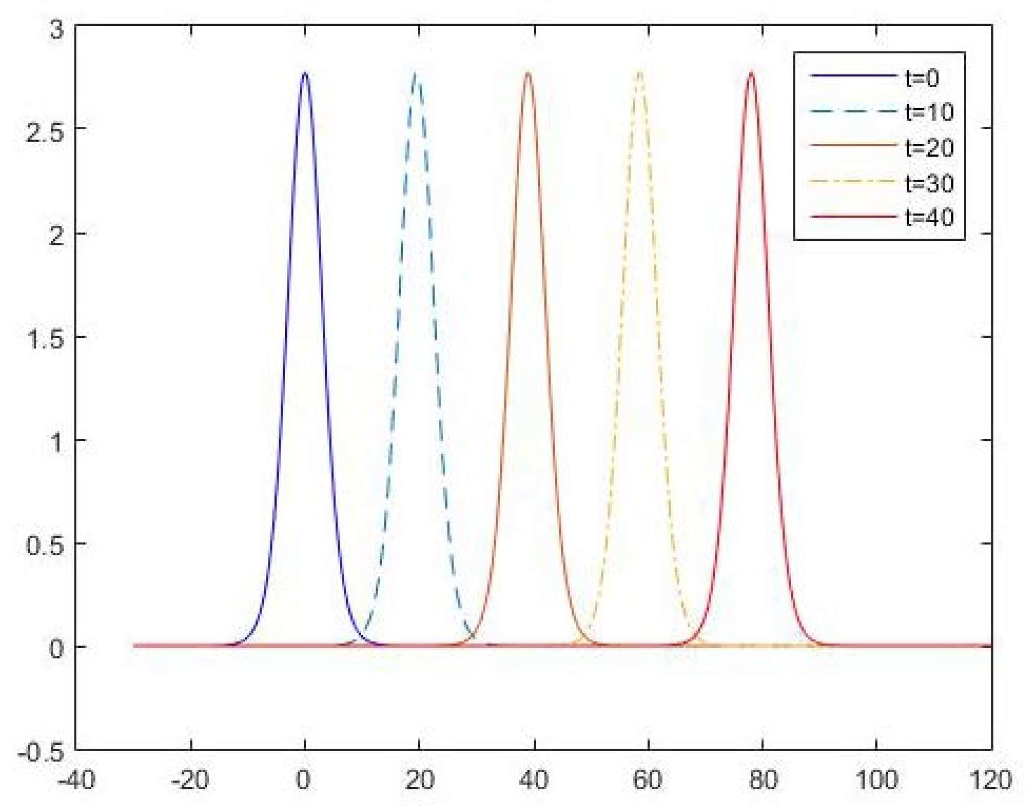
For the two-level difference scheme (21)–(23), the changes in the numerical solution $U_j^n$ at different times t when $\tau =0.05$ and $h=0.05$ are exhibited in Figure 1. It can be seen from Figure 1 that the solitary wave has not changed in shape with time t.

For various values of $\tau$ and h,

Table 1. The error estimates of the numerical solutions for scheme (21)–(23).

	${\mathbf{\parallel }\mathit{e}\mathbf{\parallel }}_{\mathsf{\infty }}$			$\mathbf{\parallel }\mathit{e}\mathbf{\parallel }$
	$\mathit{\tau }=0.2$	$\mathit{\tau }=0.05$	$\mathit{\tau }=0.0125$	$\mathit{\tau }=0.2$	$\mathit{\tau }=0.05$	$\mathit{\tau }=0.0125$
	$\mathit{h}=0.1$	$\mathit{h}=0.05$	$\mathit{h}=0.025$	$\mathit{h}=0.1$	$\mathit{h}=0.05$	$\mathit{h}=0.125$
t = 10	2.63467 × 10−2	1.65735 × 10−3	9.94049 × 10−5	7.00687 × 10−2	4.40715 × 10−3	2.54754 × 10−4
t = 20	5.05143 × 10−2	3.17890 × 10−3	1.75745 × 10−4	1.35375 × 10−1	8.51817 × 10−3	4.51715 × 10−4
t = 30	7.45117 × 10−2	4.69031 × 10−3	2.37401 × 10−4	2.00088 × 10−1	1.25923 × 10−2	6.08385 × 10−4
t = 40	9.84930 × 10−2	6.20064 × 10−3	2.84942 × 10−4	2.64761 × 10−1	1.66644 × 10−2	7.27054 × 10−4

,

Table 2. Numerical verification of the theoretical accuracy for scheme (21)–(23).

	${\mathit{orderl}}_2$			${\mathit{orderl}}_{\mathbf{\infty }}$
	$\mathit{\tau }=0.2$	$\mathit{\tau }=0.05$	$\mathit{\tau }=0.0125$	$\mathit{\tau }=0.2$	$\mathit{\tau }=0.05$	$\mathit{\tau }=0.0125$
	$\mathit{h}=0.1$	$\mathit{h}=0.05$	$\mathit{h}=0.025$	$\mathit{h}=0.1$	$\mathit{h}=0.05$	$\mathit{h}=0.125$
t = 10	–	3.99067	4.05942	–	3.99085	4.11267
t = 20	–	3.99009	4.17697	–	3.99027	4.23706
t = 30	–	3.98971	4.30429	–	3.99002	4.37191
t = 40	–	3.98953	4.44368	–	3.98985	4.51856

and

Table 3. Conservative quantity (24) for scheme (21)–(23).

	$\mathit{\tau }=0.2$	$\mathit{\tau }=0.05$	$\mathit{\tau }=0.0125$
	$\mathit{h}=0.1$	$\mathit{h}=0.05$	$\mathit{h}=0.025$
t = 0	21.67925836181	21.67925836040	21.67925835969
t = 10	21.67925803228	21.67925803744	21.67931092312
t = 20	21.67925095503	21.67925849815	21.67936576362
t = 30	21.67900791772	21.67924382931	21.67941983441
t = 40	21.67952193450	21.67927604434	21.67947672631

present the errors in the numerical solution, the results of the accuracy tests, and the discrete conserved quantities at different time levels, respectively. It is worth noting that Table 2 specifically focuses on verifying the order of spatial accuracy. Indeed, the definitions of the error norms $order{l}_2$ and $order{l}_{\infty }$ demonstrate that confirming the fourth-order spatial accuracy inherently validates the second-order temporal accuracy as well.

Remark 3.

When we consider numerical verification of the theoretical accuracy for both schemes, the order is obtained through pairwise comparison. Since there are no comparable data in the first column, there are blank values in Table 2.

4.2. The Numerical Results of Scheme (53)–(55)

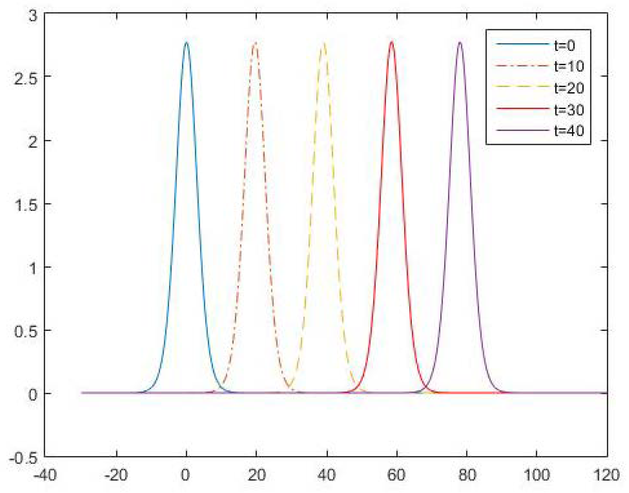
Similarly, to verify the effectiveness of the numerical scheme (53)–(55), we also plotted waveforms of the numerical solution based on (53)–(55) at different times t when $\tau =0.05$ and $h=0.05$, as in Figure 2.

The errors in the numerical solutions and the accuracy tests for the three-level difference scheme (53)–(55) at various times are shown in

Table 4. The error estimates of the numerical solutions for scheme (53)–(55).

	${\mathbf{\parallel }\mathit{e}\mathbf{\parallel }}_{\mathsf{\infty }}$			$\mathbf{\parallel }\mathit{e}\mathbf{\parallel }$
	$\mathit{\tau }=0.2$	$\mathit{\tau }=0.05$	$\mathit{\tau }=0.0125$	$\mathit{\tau }=0.2$	$\mathit{\tau }=0.05$	$\mathit{\tau }=0.0125$
	$\mathit{h}=0.1$	$\mathit{h}=0.05$	$\mathit{h}=0.025$	$\mathit{h}=0.1$	$\mathit{h}=0.05$	$\mathit{h}=0.125$
t = 10	9.35198 × 10−2	5.35165 × 10−3	3.35914 × 10−4	2.49529 × 10−1	1.36134 × 10−2	8.49912 × 10−4
t = 20	2.20014 × 10−1	1.00773 × 10−2	6.24682 × 10−4	5.68603 × 10−1	2.66997 × 10−2	1.64330 × 10−3
t = 30	3.84552 × 10−1	1.52808 × 10−2	9.34444 × 10−4	9.87308 × 10−1	4.10605 × 10−2	2.49280 × 10−3
t = 40	5.86758 × 10−1	2.10901 × 10−2	1.26603 × 10−3	1.50784 × 100	5.67519 × 10−2	3.40179 × 10−3

and

Table 5. Numerical verification of the theoretical accuracy for scheme (53)–(55).

	${\mathit{orderl}}_2$			${\mathit{orderl}}_{\mathbf{\infty }}$
	$\mathit{\tau }=0.2$	$\mathit{\tau }=0.05$	$\mathit{\tau }=0.0125$	$\mathit{\tau }=0.2$	$\mathit{\tau }=0.05$	$\mathit{\tau }=0.0125$
	$\mathit{h}=0.1$	$\mathit{h}=0.05$	$\mathit{h}=0.025$	$\mathit{h}=0.1$	$\mathit{h}=0.05$	$\mathit{h}=0.125$
t = 10	–	4.12722	3.99382	–	4.19611	4.00157
t = 20	–	4.44841	4.01184	–	4.41253	4.02216
t = 30	–	4.65339	4.03147	–	4.58752	4.04191
t = 40	–	4.79813	4.05818	–	4.73167	4.06030

. Similar to Table 2, there are blank values in Table 5 because there are no comparable data in the first column.

4.3. Comparison of the Numerical Solutions

From Table 1 and Table 4, it can be seen that although both numerical schemes are linear, scheme (21)–(23) is more efficient in its computation than scheme (53)–(55) because the absolute error in the numerical solution based on scheme (21)–(23) is smaller. The reason for this is that the three-level scheme introduces more truncation errors when extrapolating. However, as stated in Remark 2, scheme (21)–(23) cannot be used for the more complex generalized Rosenau–KdV–RLW Equation (60).

In [20], Ghilouf et al. presented four different finite difference schemes with the same accuracy as the numerical scheme presented in this paper. Choose the two-level nonlinear scheme (Scheme A in [20]) and the three-level linearized compact scheme (Scheme D in [20]) and compare them with scheme (21)–(23) in this paper. Fix the time step $\tau =0.002$ and the final time $T=1$. The ${\parallel ·\parallel }_{\infty }$ norms for the corresponding absolute error when $h=0.1,0.05$, and $0.025$ are listed in

Table 6. Comparison of errors for Scheme (21)–(23), Scheme A, and Scheme D in [20] when $\tau =0.002$.

	$\mathit{h}=0.1$	$\mathit{h}=0.05$	$\mathit{h}=0.025$
Scheme (21)–(23)	9.710410 × 10−4	6.111019 × 10−5	3.814381 × 10−6
Scheme A in [20]	2.794741 × 10−3	1.817251 × 10−4	1.137030 × 10−5
Scheme D in [20]	8.370764 × 10−4	5.160025 × 10−5	3.174356 × 10−6

. From the results in Table 6, it can be seen that the two-level linearized scheme (21)–(23) in this paper is superior to the two-level nonlinear scheme (Scheme A in [20]) but slightly inferior to the three-level compact difference scheme (Scheme D in [20]) because Scheme D in [20] requires greater computational costs.

5. Conclusions

In this paper, the two difference schemes proposed for solving the initial–boundary value problem of the nonlinear Rosenau–KdV–RLW Equations (5)–(7) demonstrate satisfactory theoretical accuracy, as confirmed by various numerical experiments. The two-level scheme in particular accurately preserves conservative quantity (8). As linear schemes, both formulations offer computational advantages by eliminating the need for nonlinear iterations, thereby significantly reducing the computational costs. Moreover, the numerical methodology and the analytical techniques developed in this study, when combined with other novel analysis technology [31], can be extended to investigating more complex equations, including the generalized Rosenau–KdV–RLW equation and the Rosenau–Kawahara–RLW equation.

References

1. Korteweg, D.J.; de Vires, G. On the change of form of long waves advancing in a rectangular canal, and on a new type of long stationary waves. Philos. Mag. 1895, 39, 422–443. [Google Scholar] [CrossRef]
2. Peregrine, D.H. Calculations of the development of an undular bore. J. Fluid Mech. 1966, 25, 321–330. [Google Scholar]
3. Rosenau, P. A quasi-continuous description of a nonlinear transmission line. Phys. Scr. 1986, 34, 827–829. [Google Scholar]
4. Rosenau, P. Dynamics of dense discrete systems: High order effects. Prog. Theor. Phys. 1988, 79, 1028–1042. [Google Scholar]
5. Kim, Y.D.; Lee, H.Y. The convergence of finite element Galerkin solution for the Rosenau equation. Korean J. Comput. Appl. Math. 1998, 5, 171–180. [Google Scholar]
6. Chung, S.K.; Pani, A.K. Numerical methods for the Rosenau equation. Appl. Anal. 2001, 77, 351–369. [Google Scholar]
7. Hu, J.S.; Zheng, K.L. Two conservative difference schemes for the generalized Rosenau equation. Bound. Value Probl. 2010, 2010, 543503. [Google Scholar] [CrossRef]
8. Özer, S. Numerical solution of the Rosenau-KdV-RLW equation by operator splitting techniques based on B-spline collocation method. Numer. Methods Partial Differ. Equ. 2019, 35, 1928–1943. [Google Scholar]
9. Özer, S. Two efficient numerical methods for solving Rosenau-KdV-RLW equation. Kuwait J. Sci. 2021, 48, 14–24. [Google Scholar]
10. Razborova, P.; Moraru, L.; Biswas, A. Perturbation of dispersive shallow water waves with Rosenau-KdV-RLW equation and power law nonlinearity. Rom. J. Phys. 2014, 59, 658–676. [Google Scholar]
11. Razborova, P.; Ahmed, B.; Biswas, A. Solitons, shock waves and conservation laws of Rosenau-KdV-RLW equation with power law nonlinearity. Appl. Math. Inform. Sci. 2014, 8, 485–491. [Google Scholar]
12. Razborova, P.; Kara, A.H.; Biswas, A. Additional conservation laws for Rosenau-KdV-RLW equation with power law nonlinearity by Lie symmetry. Nonlin. Dyn. 2015, 79, 743–748. [Google Scholar]
13. Ak, T.; Karakoc, S.B.G.; Biswas, A. Numerical scheme to dispersive shallow water waves. J. Comput. Theor. Nanos. 2016, 13, 7084–7092. [Google Scholar]
14. Kaur, A.; Kanwar, V.; Ramos, H. A conservative algorithm based on a hybrid block method and tension B-spline differential quadrature method for Rosenau–KdV–RLW equation. Math. Meth. Appl. Sci. 2024, 47, 8638–8650. [Google Scholar]
15. Korkmaz, B.; Dereli, Y. Numerical solution of the Rosenau-KdV-RLW equation by using RBFs collocation method. Int. J. Mod. Phys. C 2016, 27, 1650117. [Google Scholar]
16. Ahmat, M.; Qiu, J. Compact ETDRK scheme for nonlinear dispersive wave equations. Comput. Appl. Math. 2021, 40, 286. [Google Scholar]
17. Shallu; Kukreja, V.K. An efficient collocation algorithm with SSP-RK43 scheme to solve Rosenau-KdV-RLW equation. Int. J. Appl. Comput. Math. 2021, 7, 161. [Google Scholar]
18. Pan, X.T.; Wang, Y.J.; Zhang, L.M. Numerical analysis of a pseudo-compact C-N conservative scheme for the Rosenau-KdV equation coupling with the Rosenau-RLW equation. Bound. Value Probl. 2015, 2015, 65. [Google Scholar]
19. Wongsaijai, B.; Poochinapan, K. A three-level average implicit finite difference scheme to solve equation obtained by coupling the Rosenau-KdV equation and the Rosenau-RLW equation. Appl. Math. Comput. 2014, 245, 289–304. [Google Scholar]
20. Ghiloufi, A.; Omrani, K. New conservative difference schemes with fourth-order accuracy for some model equation for nonlinear dispersive waves. Numer. Methods Partial. Differ. Equ. 2018, 34, 451–500. [Google Scholar]
21. Labidi, S.; Rahmeni, M.; Omrani, K. Numerical approach of dispersive shallow water waves with Rosenau-KdV-RLW equation in (2 + 1)-dimensions. Discret. Cont. Dyn.-S 2023, 16, 2157–2176. [Google Scholar] [CrossRef]
22. Wang, X.F.; Dai, W.Z. A three-level linear implicit conservative scheme for the Rosenau-KdV-RLW equation. J. Comput. Appl. Math. 2018, 330, 295–306. [Google Scholar]
23. Verma, A.K.; Rawani, M.K. Numerical solutions of generalized Rosenau-KDV-RLW equation by using Haar wavelet collocation approach coupled with nonstandard finite difference scheme and quasilinearization. Numer. Methods Partial Differ. Equ. 2023, 39, 1085–1107. [Google Scholar] [CrossRef]
24. Zhou, Y.L. Application of Discrete Functional Analysis to the Finite Difference Method; International Academic Publishers: Beijing, China, 1990. [Google Scholar]
25. Zheng, K.L.; Hu, J.S. High-order conservative Crank-Nicolson scheme for regularized long wave equation. Adv. Differ. Equ. 2013, 2013, 287. [Google Scholar]
26. Shumoua, F.A.; Fatimah, A.A.; Hany, N.H. An efficient numerical technique for investigating the generalized Rosenau-KDV-RLW equation by using the Fourier spectral method. AIMS Math. 2024, 9, 8661–8688. [Google Scholar]
27. Li, S.; Kravchenko, O.V.; Qu, K. On the L convergence of a novel fourth-order compact and conservative difference scheme for the generalized Rosenau-KdV-RLW equation. Numer. Algorithms 2023, 94, 789–816. [Google Scholar] [CrossRef]
28. Aydin, A. A convergent two-level linear scheme for the generalized Rosenau-KdV-RLW equation. Turk. J. Math. 2019, 43, 2226–2245. [Google Scholar] [CrossRef]
29. Cai, J.X.; Hong, Q.; Yang, B. Local structure-preserving methods for the generalized Rosenau-RLW-KdV equation with power law nonlinearity. Chin. Phys. B 2017, 26, 100202. [Google Scholar]
30. Wang, X.F.; Dai, W.Z. A new conservative finite difference scheme for the generalized Rosenau-KdV-RLW equation. Comput. Appl. Math. 2020, 39, 237. [Google Scholar]
31. Nas, M.; Yalçın, S.; Bayram, H. A class of analytic functions defined by a second order differential inequality and error function. Int. J. Appl. Comput. Math. 2024, 10, 42. [Google Scholar] [CrossRef]
Figure 1. Numerical solutions of u ( x , t ) according to scheme (21)–(23) with τ = 0.05 , h = 0.05 .
Symmetry 17 00566 g001
Figure 2. Numerical solutions of u ( x , t ) according to scheme (53)–(55) with τ = 0.05 , h = 0.05 .
Symmetry 17 00566 g002