Characteristic Analysis of Local Wave Solutions for the (21)-Dimensional Asymmetric Nizhnik–Novikov–Veselov Equation

Abstract

This study investigates the (2+1)-dimensional asymmetric Nizhnik–Novikov–Veselov (ANNV) equation, a significant model in nonlinear science, using the Kadomtsev–Petviashvili (KP) hierarchy reduction method. Despite the extensive research on the ANNV equation, a comprehensive exploration of its solutions using the KP hierarchy reduction method is lacking. This gap is addressed by identifying constraint conditions that transform a specific KP hierarchy equation into the ANNV equation, thereby enabling the derivation of its Gram determinant solutions. By selecting appropriate $\tau$ functions, we obtain breather solutions and analyze their dynamic behavior during wave oscillations. Additionally, lump solutions are derived through long-wave limit analysis, revealing their unique characteristics. This study further explores hybrid solutions that combine breathers and lumps, providing new insights to the interaction between these localized wave phenomena. Our findings enhance the understanding of the ANNV equation’s dynamics and contribute to the broader field of nonlinear wave theory.

1. Introduction

Nonlinear science, an interdisciplinary domain, has garnered growing interest in modern research. Advances in technology and science have highlighted the complexity and dynamic nature of natural phenomena, emphasizing the importance of nonlinear systems. Theoretical and methodological developments in nonlinear science offer precise and detailed frameworks for the analysis of diverse phenomena, such as water waves, nonlinear optics, plasma physics, and biological processes. Addressing nonlinear systems poses substantial challenges, yet integrable systems stand out due to their solvability. Prominent integrable equations include the Korteweg–de Vries (KdV) equation [1], Kadomtsev–Petviashvili (KP) equation [2], Camassa–Holm equation [3], Benjamin–Ono equation [4], and Davey–Stewartson (DS) system [5]. These equations serve as foundational models in understanding nonlinear dynamics and find application across various scientific and engineering disciplines.

Localized wave solutions are pivotal in the study of integrable systems, with solitons, breathers, and lumps being the most common types. These solutions are essential in understanding complex dynamics in nonlinear systems. Solitons are stable waves that retain their form and energy as they travel through a medium. Breathers are periodic waves localized in time or space, while lumps are localized waves that diminish in all directions. To solve integrable systems, researchers have developed several methods, such as the inverse scattering transform (IST) [6,7], Bäcklund transformation (BT) [8,9,10], Darboux transformation (DT) [11,12], Riemann–Hilbert approach [13,14], Hirota bilinear method (HBM) [15,16,17], and KP hierarchy reduction method (KPHRM) [18].

This study examines the (2+1)-dimensional integrable asymmetrical Nizhnik–Novikov–Veselov (ANNV) equation [19]

$$\begin{array}{c}\hfill u_t+u_{xxx}+3{(u\int u_x\mathrm{d}y)}_x=0,\end{array}$$

(1)

where u is a function of the spatial coordinates $x,y$ and time t, with the subscripts denoting partial derivatives. By applying the transformation

$$\begin{array}{c}\hfill u=u_0+2{(lnf)}_{xy},\end{array}$$

(2)

with $u_0=-1$, (1) is converted into

$$\begin{array}{c}\hfill (D_y{D}_t+D_x^3{D}_y-3D_x^2)f·f=0,\end{array}$$

(3)

where the operator D [15] is given by

$$\begin{array}{c}\hfill D_x^m{D}_y^n{D}_t^p(a·b)={({\partial }_x-{\partial }_{x^{\prime }})}^m{({\partial }_y-{\partial }_{y^{\prime }})}^n{({\partial }_t-{\partial }_{t^{\prime }})}^{p}a(x,y,t)b(x^{\prime },y^{\prime },t^{\prime }){|}_{x=x^{\prime },y=y^{\prime },t=t^{\prime }}.\end{array}$$

(4)

The ANNV equation, proposed by Boiti et al. [20], is a mathematical model for incompressible fluid dynamics and is derived from the symmetry constraint of the KP equation [21]. Extensive research has been conducted on the exact solutions of (1). For instance, Zhao et al. [22] used the HBM and the long-wave limit method to construct resonance Y-type solitons and hybrid solutions. Liu and Wen [23] derived soliton, breather, and lump solutions using the HBM. Guo et al. [24] obtained rational and semi-rational solutions via the binary DT. Wu and Guo [25] explored exact solutions using the extended Jacobian elliptic function expansion method. Guo et al. [26] constructed localized solutions in both time and space using the binary DT. Zhang and Liu [27] derived various localized wave solutions by obtaining the BT for (1) and applying the extended homogeneous balance method.

Our research has identified a notable gap in the literature: no previous studies have applied the KPHRM to construct exact solutions for (1). This method, originally developed in the 1980s by Mikio Sato and colleagues from the Kyoto school within the context of KP theory [28,29,30], is designed to derive localized wave solutions for nonlinear evolution equations. It capitalizes on the connection between soliton solutions of the KP hierarchy and those of the target equations. By treating the target equation as a special reduction of integrable equations within the KP hierarchy, this method uses $\tau$-function solutions to construct exact solutions for various nonlinear models. Significant progress has been made in applying the KPHRM to a variety of equations. For example, Ohta et al. [31] have used it to study dark soliton interactions in the focusing–defocusing NLS equation. Ohta and Yang have explored higher-order rogue wave solutions of the NLS [32] and line rogue wave solutions of the DS equation [33,34]. Similarly, the Tian team [35,36,37] has obtained solitary wave, periodic wave, and rogue wave solutions for variable coefficient equations using this method. Additionally, solutions for (3+1)-dimensional nonlinear evolution equations, including multiple dark solitons and semi-rational solutions, have been successfully constructed [38,39] Given these advancements, the primary objective of our paper is to apply the KPHRM to solve (1), with a particular focus on deriving breather, lump, and hybrid solutions.

This paper is organized as follows. In Section 2, the KPHRM is introduced, which transforms specific equations from the KP hierarchy into the bilinear form of the ANNV equation. This section lays the groundwork for the derivation of various localized wave solutions. In Section 3, the localized wave solutions of the ANNV equation are investigated, including soliton, breather, lump, and hybrid solutions. These solutions are derived using the Gram determinant method and the KPHRM. In Section 4, a modulation stability analysis of the ANNV equation is conducted, demonstrating that it does not support rogue wave solutions. This analysis provides insights into the stability properties of the equation. In Section 5, the study is concluded by summarizing the key findings and contributions, highlighting the significance of the results in the broader context of nonlinear wave theory.

2. KP Hierarchy Reduction Method

The core idea of the KPHRM is to reduce a certain equation in the KP hierarchy to a specific nonlinear partial differential equation by appropriate constraints. This approach takes advantage of the integrability of the KP hierarchy to represent the solution via the $\tau$ function. The function $\tau$ is a key object in the KP hierarchy, which satisfies a sequence of bilinear equations. Various local wave solutions, such as soliton, breathing wave, and lump solutions, can be constructed by choosing an appropriate $\tau$ function. The following are the specific steps required to apply the KPHRM to the ANNV equation.

First, a suitable KP hierarchy equation is chosen as a starting point. For example, consider the second equation in the KP hierarchy,

$$(D_{x_1}^3{D}_{x_2}+2D_{x_3}{D}_{x_2}-3D_{x_1}{D}_{x_4}){\tau }_n·{\tau }_n=0,$$

(5)

where D denotes the Hirota bilinear operator.

Next, the constraint conditions that transform the KP hierarchy equation into (1) are established. These conditions typically involve variable transformations and specific conditions for dimensionality reduction. For example, by choosing appropriate constraint conditions,

$$\begin{array}{c}\hfill ({\partial }_{x_1}+{\partial }_{x_4})\tau =c\tau ,x_1=\mathrm{I}x,x_2=\mathrm{I}y,x_3=-2\mathrm{I}t,\end{array}$$

(6)

or

$$\begin{array}{c}\hfill ({\partial }_{x_1}-{\partial }_{x_4})\tau =c\tau ,x_1=x,x_2=y,x_3=2t,\end{array}$$

(7)

where ${\mathrm{I}}^2=-1$. When ${\tau }_0=f$, the KP hierarchy Equation (5) reduces to (3).

Construct $\tau$ functions that satisfy the above constraints. The $\tau$ function is represented as a Gram determinant,

$${\tau }_n=\underset{1⩽i,j⩽N}{det}\left(G_{ij}^{\left(n\right)}\right),$$

(8)

where $G_{ij}^{\left(n\right)}$ satisfies the relations

$$\begin{array}{cc}\hfill & {\partial }_{x_1}{G}_{ij}^{\left(n\right)}=a_i^{\left(n\right)}{b}_j^{\left(n\right)},\hfill \\ \hfill & {\partial }_{x_2}{G}_{ij}^{\left(n\right)}=a_i^{(n+1)}{b}_j^{\left(n\right)}+a_i^{\left(n\right)}{b}_j^{(n-1)},\hfill \\ \hfill & {\partial }_{x_3}{G}_{ij}^{\left(n\right)}=a_i^{(n+2)}{b}_j^{\left(n\right)}+a_i^{(n+1)}{b}_j^{(n-1)}+a_i^{\left(n\right)}{b}_j^{(n-2)},\hfill \\ \hfill & {\partial }_{x_4}{G}_{ij}^{\left(n\right)}=a_i^{(n+3)}{b}_j^{\left(n\right)}+a_i^{(n+2)}{b}_j^{(n-1)}+a_i^{(n+1)}{b}_j^{(n-2)}+a_i^{\left(n\right)}{b}_j^{(n-3)},\hfill \\ \hfill & G_{ij}^{(n+1)}=G_{ij}^{\left(n\right)}+a_i^{\left(n\right)}{b}_j^{(n+1)},\hfill \\ \hfill & {\partial }_{x_k}{a}_i^{\left(n\right)}=a_i^{(n+k)},{\partial }_{x_k}{b}_j^{\left(n\right)}=-b_j^{(n-k)},k=1,2,3,4,\hfill \end{array}$$

(9)

where $a_i^{\left(n\right)}$ and $b_j^{\left(n\right)}$ are functions of $x_1$, $x_2$, $x_3$ and $x_4$. The proof for the Gram determinant solution of Equation (5) is detailed in ref. [40]. In the proof process, several key expressions are utilized to derive the necessary results. Firstly, we consider the partial derivative of the determinant with respect to x,

$${\partial }_x\underset{1⩽i,j⩽N}{det}\left(m_{ij}\right)={\Sigma }_{i,j=1}^N{\Delta }_{ij}{\partial }_x{a}_{ij},$$

(10)

and we employ the bordered determinant, which is defined as

$${\tau }_n=\underset{1⩽i,j⩽N}{det}\left(G_{ij}^{\left(n\right)}\right),$$

(11)

where ${\Delta }_{ij}$ denotes the algebraic cofactor of the element $a_{ij}$ in the matrix. These expressions play a crucial role in the proof, providing a systematic approach to verifying that the $\tau$-function satisfies the required bilinear equations.

Various local wave solutions of (1) can be derived by choosing an appropriate $\tau$ function. For example, by choosing an appropriate $\tau$ function, soliton solutions, breather solutions, lump solutions, and their hybrid solutions can be obtained. The dynamic behavior of these solutions can be investigated by numerical simulations and theoretical analysis.

3. Local Wave Solutions

Local wave solutions hold a pivotal position in nonlinear science and are broadly applicable in fluid dynamics, nonlinear optics, and plasma physics. The analysis of the dynamics of these solutions is crucial in understanding the underlying mechanisms and behaviors of nonlinear systems [41,42,43]. This section will meticulously examine the local wave solutions of (1), encompassing soliton, breather, and lump solutions and their hybrid configurations.

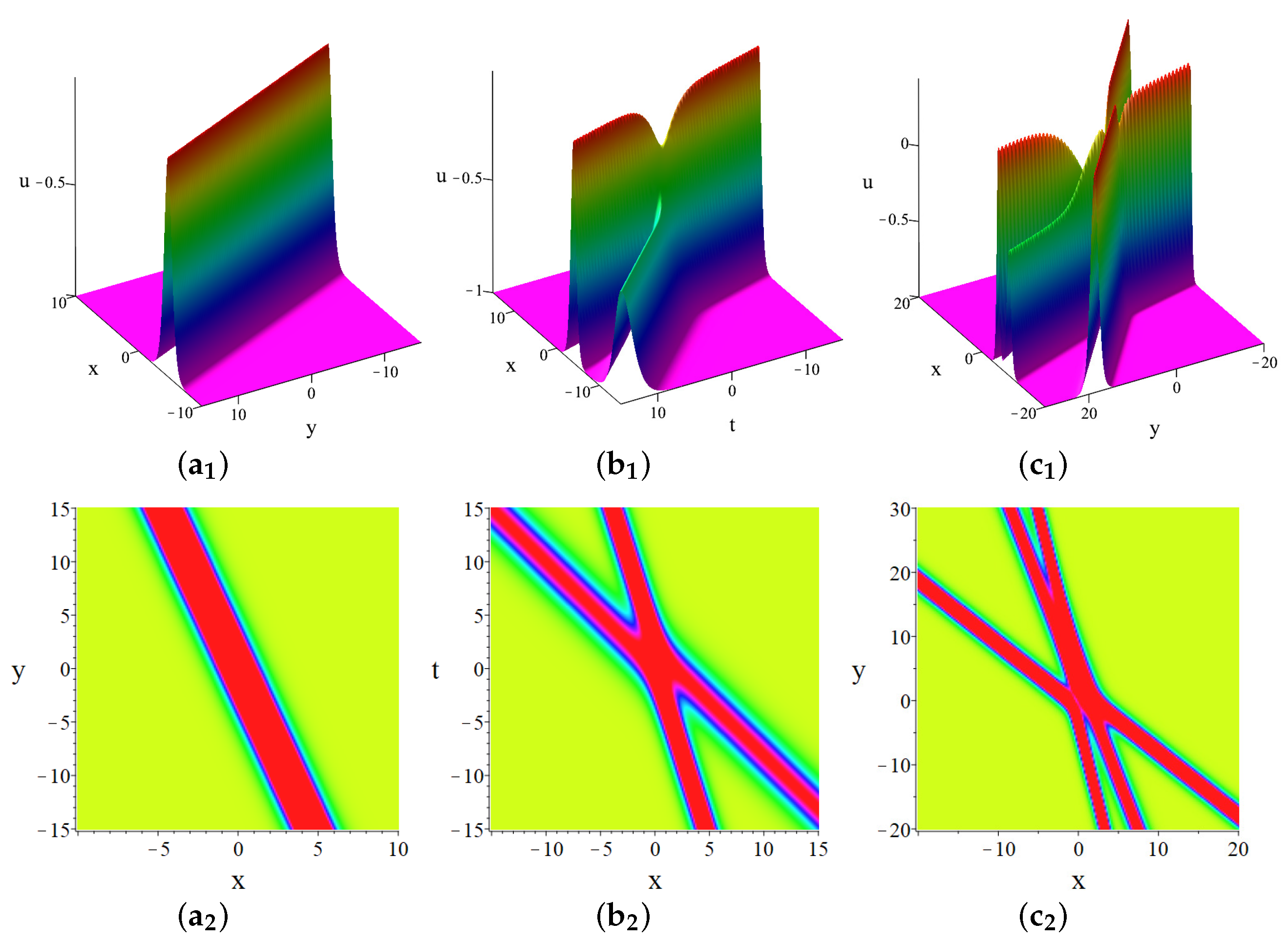
3.1. Soliton Solutions

To investigate the multi-soliton solutions of (1), we select specific functions $G_{ij}^{\left(n\right)}$, $a_i^{\left(n\right)}$ and $b_j^{\left(n\right)}$ as follows:

$$\begin{array}{cc}\hfill & G_{ij}^{\left(n\right)}={\gamma }_{ij}+{\displaystyle \frac{1}{{\mu }_i+{\nu }_j}}{a}_i^{\left(n\right)}{b}_j^{\left(n\right)},\hfill \\ \hfill & a_i^{\left(n\right)}={\mu }_i^n({\mu }_i+{\nu }_i){\mathrm{e}}^{{\xi }_i},\hfill \\ \hfill & b_j^{\left(n\right)}={(-\frac{1}{{\nu }_j})}^{\left(n\right)}{\mathrm{e}}^{{\eta }_j},\hfill \end{array}$$

(12)

with

$$\begin{array}{cc}\hfill & {\xi }_i={\mu }_i{x}_1+{\mu }_i^2{x}_2+{\mu }_i^3{x}_3+{\mu }_i^4{x}_4+{\xi }_i^0,\hfill \\ \hfill & {\eta }_j={\nu }_j{x}_1-{\nu }_j^2{x}_2+{\nu }_j^3{x}_3-{\nu }_j^4{x}_4+{\eta }_j^0,\hfill \end{array}$$

(13)

where ${\mu }_i$, ${\nu }_j$ are constants, and ${\xi }_i^0,{\eta }_j^0$ are real constants. The parameter ${\gamma }_{ij}$ is defined to be 1 when $i=j$ and 0 otherwise. With these definitions and (7), the determinant f can be expressed as

$$f={\tau }_0={\left|{\gamma }_{ij}+{\displaystyle \frac{{\mu }_i+{\nu }_i}{{\mu }_i+{\nu }_j}}{\mathrm{e}}^{{\xi }_i+{\eta }_j}\right|}_{N\times N},$$

(14)

with

$$\begin{array}{cc}\hfill & {\xi }_i={\mu }_{i}x+{\mu }_i^{2}y+2{\mu }_i^{3}t+{\xi }_i^0,\hfill \\ \hfill & {\eta }_j={\nu }_{j}x-{\nu }_j^{2}y+2{\nu }_j^{3}t+{\eta }_j^0,\hfill \end{array}$$

(15)

where the condition $({\mu }_i+{\nu }_j)-({\mu }_i^4-{\nu }_j^4)=0$ must be satisfied. By applying the logarithmic transformation

$$u=-1+2{(lnf)}_{xy},$$

(16)

we can derive the multi-soliton solutions u of (1).

For $N=1$, the solution corresponds to a single soliton:

$$f=1+{\mathrm{e}}^{{\xi }_1+{\eta }_1},$$

(17)

with

$$\begin{array}{cc}\hfill & {\xi }_1={\mu }_{1}x+{\mu }_1^{2}y+2{\mu }_1^{3}t+{\xi }_1^0,\hfill \\ \hfill & {\eta }_1={\nu }_{1}x-{\nu }_1^{2}y+2{\nu }_1^{3}t+{\eta }_1^0.\hfill \end{array}$$

(18)

Here, ${\mu }_1$ is an arbitrary constant, while ${\xi }_1^0$ and ${\eta }_1^0$ are real constants representing initial phases. The parameter ${\gamma }_{11}$ is set to be 1. Additionally, setting ${\mu }_1=\sqrt{2}$, the value of ${\nu }_1$ is determined by the condition $({\mu }_1+{\nu }_1)-({\mu }_1^4-{\nu }_1^4)=0$, which yields ${\displaystyle \frac{1}{6}}{\left(160\sqrt{2}-108+12\sqrt{465-240\sqrt{2}}\right)}^{{\displaystyle \frac{1}{3}}}-{\displaystyle \frac{8}{3{\left(160\sqrt{2}-108+12\sqrt{465-240\sqrt{2}}\right)}^{\frac{1}{3}}}}+{\displaystyle \frac{1}{3}}\sqrt{2}$. Substituting f into (16), we obtain the one-soliton solution for (1):

$$u=-1+{\displaystyle \frac{{({\mu }_1+{\nu }_1)}^2({\mu }_1-{\nu }_1)}{2}}{\mathrm{sech}}^2{\displaystyle \frac{1}{2}}({\xi }_1+{\eta }_1).$$

(19)

This solution describes a localized wave that propagates without changing its shape. A graphical representation of this solution (19) is shown in Figure 1${\mathrm{a}}_1$,${\mathrm{a}}_2$. It exhibits distinct physical properties in both the x- and y-directions. In the x-direction, the soliton has an amplitude of ${\displaystyle \frac{{({\mu }_1+{\nu }_1)}^2({\mu }_1-{\nu }_1)}{2}}$, a width of ${\displaystyle \frac{2}{{\mu }_1+{\nu }_1}}$, and a velocity of ${\displaystyle \frac{4({\mu }_1^3+{\nu }_1^3)}{{\mu }_1+{\nu }_1}}$. Its wave number is ${\displaystyle \frac{{\mu }_1+{\nu }_1}{2}}$, and the primary phase is ${\xi }_1^0+{\eta }_1^0$. In the y-direction, the amplitude remains ${\displaystyle \frac{{({\mu }_1+{\nu }_1)}^2({\mu }_1-{\nu }_1)}{2}}$, but the width changes to ${\displaystyle \frac{2}{{\mu }_1+{\nu }_1}}$ and the velocity to ${\displaystyle \frac{4({\mu }^3+{\nu }_1^3)}{{\mu }_1+{\nu }_1}}$. The wave number in this direction is ${\displaystyle \frac{{\mu }_1+{\nu }_1}{2}}$, with the same primary phase ${\xi }_1^0+{\eta }_1^0$. These properties highlight the key characteristics of the one-soliton solution, demonstrating its stability and propagation behavior in different spatial directions.

For $N=2$, the two-soliton solution is formulated via the Gram determinant:

$$\begin{array}{cc}\hfill f& =\left|\begin{array}{cc}1+{\mathrm{e}}^{{\xi }_1+{\eta }_1}& {\displaystyle \frac{{\mu }_1+{\nu }_1}{{\mu }_1+{\nu }_2}}{\mathrm{e}}^{{\xi }_1+{\eta }_2}\\ {\displaystyle \frac{{\mu }_2+{\nu }_2}{{\mu }_2+{\nu }_1}}{\mathrm{e}}^{{\xi }_2+{\eta }_1}& 1+{\mathrm{e}}^{{\xi }_2+{\eta }_2}\end{array}\right|.\hfill \end{array}$$

(20)

Expanding this determinant, we obtain

$$\begin{array}{c}\hfill f=1+{\mathrm{e}}^{{\xi }_1+{\eta }_1}+{\mathrm{e}}^{{\xi }_2+{\eta }_2}+\left(1-{\displaystyle \frac{{\mu }_1+{\nu }_1}{{\mu }_1+{\nu }_2}}{\displaystyle \frac{{\mu }_2+{\nu }_2}{{\mu }_2+{\nu }_1}}\right){\mathrm{e}}^{{\xi }_1+{\eta }_1+{\xi }_2+{\eta }_2},\end{array}$$

(21)

with

$$\begin{array}{cc}\hfill & {\xi }_i={\mu }_{i}x+{\mu }_i^{2}y+2{\mu }_i^{3}t+{\xi }_i^0,\hfill \\ \hfill & {\eta }_i={\nu }_{i}x-{\nu }_i^{2}y+2{\nu }_i^{3}t+{\eta }_i^0,i=1,2.\hfill \end{array}$$

(22)

Here, ${\mu }_1$, ${\mu }_2$, ${\nu }_1$, ${\nu }_2$, ${\xi }_1^0$, ${\xi }_2^0$, ${\eta }_1^0$, ${\eta }_2^0$ are real constants. The two-soliton solution u can be visually observed in Figure 1${\mathrm{b}}_1$,${\mathrm{b}}_2$.

To verify the elasticity of the soliton collision, we analyze the dynamical behavior of the solution in the asymptotic limits of large positive and negative times. Consider the scenario where the soliton velocity is ${\displaystyle \frac{4({\mu }_1^3+{\nu }_1^3)}{{\mu }_1+{\nu }_1}}$ and ${\xi }_1+{\eta }_1$ is held constant. As $t\to +\infty$, ${\xi }_2+{\eta }_2\to +\infty$, leading to $e^{{\xi }_2+{\eta }_2}\to +\infty$. Consequently, f behaves as

$$f\sim e^{{\xi }_2+{\eta }_2}+\left(1-{\displaystyle \frac{{\mu }_1+{\nu }_1}{{\mu }_1+{\nu }_2}}{\displaystyle \frac{{\mu }_2+{\nu }_2}{{\mu }_2+{\nu }_1}}\right)e^{{\xi }_1+{\eta }_1+{\xi }_2+{\eta }_2}.$$

Under this condition, the two-soliton solution approximates to

$$u\sim -1+{\displaystyle \frac{{({\mu }_1+{\nu }_1)}^2({\mu }_1-{\nu }_1)}{2}}{\mathrm{sech}}^2\left({\displaystyle \frac{1}{2}}\left({\xi }_1+{\eta }_1+ln\left(1-{\displaystyle \frac{{\mu }_1+{\nu }_1}{{\mu }_1+{\nu }_2}}{\displaystyle \frac{{\mu }_2+{\nu }_2}{{\mu }_2+{\nu }_1}}\right)\right)\right).$$

Similarly, as $t\to -\infty$, ${\xi }_2+{\eta }_2\to -\infty$, causing $e^{{\xi }_2+{\eta }_2}\to 0$. Thus, we have

$$f\sim 1+e^{{\xi }_1+{\eta }_1}.$$

In this scenario, the two-soliton solution converges to

$$u\sim -1+{\displaystyle \frac{{({\mu }_1+{\nu }_1)}^2({\mu }_1-{\nu }_1)}{2}}{\mathrm{sech}}^2\left({\displaystyle \frac{1}{2}}({\xi }_1+{\eta }_1)\right).$$

Next, consider the coordinate system where the soliton velocity is ${\displaystyle \frac{4({\mu }_2^3+{\nu }_2^3)}{{\mu }_2+{\nu }_2}}$ and ${\xi }_2+{\eta }_2$ is held constant. As $t\to +\infty$, ${\xi }_1+{\eta }_1\to -\infty$, leading to $e^{{\xi }_1+{\eta }_1}\to 0$. Thus, we have

$$f\sim 1+e^{{\xi }_2+{\eta }_2}.$$

Here, the two-soliton solution approximates to

$$u\sim -1+{\displaystyle \frac{{({\mu }_2+{\nu }_2)}^2({\mu }_2-{\nu }_2)}{2}}{\mathrm{sech}}^2\left({\displaystyle \frac{1}{2}}({\xi }_2+{\eta }_2)\right).$$

Finally, as $t\to -\infty$, ${\xi }_1+{\eta }_1\to +\infty$, causing $e^{{\xi }_1+{\eta }_1}\to +\infty$. Thus, we have

$$f\sim e^{{\xi }_1+{\eta }_1}+\left(1-{\displaystyle \frac{{\mu }_1+{\nu }_1}{{\mu }_1+{\nu }_2}}{\displaystyle \frac{{\mu }_2+{\nu }_2}{{\mu }_2+{\nu }_1}}\right)e^{{\xi }_1+{\eta }_1+{\xi }_2+{\eta }_2}.$$

Thus, the two-soliton solution tends to

$$u\sim -1+{\displaystyle \frac{{({\mu }_2+{\nu }_2)}^2({\mu }_2-{\nu }_2)}{2}}{\mathrm{sech}}^2\left({\displaystyle \frac{1}{2}}\left({\xi }_2+{\eta }_2+ln\left(1-{\displaystyle \frac{{\mu }_1+{\nu }_1}{{\mu }_1+{\nu }_2}}{\displaystyle \frac{{\mu }_2+{\nu }_2}{{\mu }_2+{\nu }_1}}\right)\right)\right).$$

In conclusion, the interaction between the two solitons results in the solitons retaining their speeds and amplitudes, albeit with a phase shift of $ln\left(1+{\displaystyle \frac{{\mu }_1+{\nu }_1}{{\mu }_1+{\nu }_2}}{\displaystyle \frac{{\mu }_2+{\nu }_2}{{\mu }_2+{\nu }_1}}\right)$. This confirms that the collision is elastic.

For $N=3$, the three-soliton solution is

$$\begin{array}{cc}\hfill f& =\left|\begin{array}{ccc}1+{\mathrm{e}}^{{\xi }_1+{\eta }_1}& {\displaystyle \frac{{\mu }_1+{\nu }_1}{{\mu }_1+{\nu }_2}}{\mathrm{e}}^{{\xi }_1+{\eta }_2}& {\displaystyle \frac{{\mu }_1+{\nu }_1}{{\mu }_1+{\nu }_3}}{\mathrm{e}}^{{\xi }_1+{\eta }_3}\\ {\displaystyle \frac{{\mu }_2+{\nu }_2}{{\mu }_2+{\nu }_1}}{\mathrm{e}}^{{\xi }_2+{\eta }_1}& 1+{\mathrm{e}}^{{\xi }_2+{\eta }_2}& {\displaystyle \frac{{\mu }_2+{\nu }_2}{{\mu }_2+{\nu }_3}}{\mathrm{e}}^{{\xi }_2+{\eta }_3}\\ {\displaystyle \frac{{\mu }_3+{\nu }_3}{{\mu }_3+{\nu }_1}}{\mathrm{e}}^{{\xi }_3+{\eta }_1}& {\displaystyle \frac{{\mu }_3+{\nu }_3}{{\mu }_3+{\nu }_2}}{\mathrm{e}}^{{\xi }_3+{\eta }_2}& 1+{\mathrm{e}}^{{\xi }_3+{\eta }_3}\end{array}\right|.\hfill \end{array}$$

(23)

Expanding this determinant, we obtain

$$\begin{array}{cc}\hfill f=& 1+{\mathrm{e}}^{{\xi }_1+{\eta }_1}+{\mathrm{e}}^{{\xi }_2+{\eta }_2}+{\mathrm{e}}^{{\xi }_3+{\eta }_3}+\left(1-{\displaystyle \frac{{\mu }_2+{\nu }_2}{{\mu }_2+{\nu }_1}}{\displaystyle \frac{{\mu }_1+{\nu }_1}{{\mu }_1+{\nu }_2}}\right){\mathrm{e}}^{{\xi }_1+{\eta }_1+{\xi }_2+{\eta }_2}\hfill \\ \hfill & +\left(1-{\displaystyle \frac{{\mu }_1+{\nu }_1}{{\mu }_1+{\nu }_3}}{\displaystyle \frac{{\mu }_3+{\nu }_3}{{\mu }_3+{\nu }_1}}\right){\mathrm{e}}^{{\xi }_1+{\eta }_1+{\xi }_3+{\eta }_3}+\left(1-{\displaystyle \frac{{\mu }_2+{\nu }_2}{{\mu }_2+{\nu }_3}}{\displaystyle \frac{{\mu }_3+{\nu }_3}{{\mu }_3+{\nu }_2}}\right){\mathrm{e}}^{{\xi }_2+{\eta }_2+{\xi }_3+{\eta }_3}\hfill \\ \hfill & +\left(1-{\displaystyle \frac{{\mu }_2+{\nu }_2}{{\mu }_2+{\nu }_1}}{\displaystyle \frac{{\mu }_1+{\nu }_1}{{\mu }_1+{\nu }_2}}-{\displaystyle \frac{{\mu }_1+{\nu }_1}{{\mu }_1+{\nu }_3}}{\displaystyle \frac{{\mu }_3+{\nu }_3}{{\mu }_3+{\nu }_1}}-{\displaystyle \frac{{\mu }_2+{\nu }_2}{{\mu }_2+{\nu }_3}}{\displaystyle \frac{{\mu }_3+{\nu }_3}{{\mu }_3+{\nu }_2}}\right.\hfill \\ \hfill & \left.+{\displaystyle \frac{{\mu }_1+{\nu }_1}{{\mu }_1+{\nu }_3}}{\displaystyle \frac{{\mu }_2+{\nu }_2}{{\mu }_2+{\nu }_1}}{\displaystyle \frac{{\mu }_3+{\nu }_3}{{\mu }_3+{\nu }_2}}+{\displaystyle \frac{{\mu }_1+{\nu }_1}{{\mu }_1+{\nu }_2}}{\displaystyle \frac{{\mu }_3+{\nu }_3}{{\mu }_3+{\nu }_1}}{\displaystyle \frac{{\mu }_2+{\nu }_2}{{\mu }_2+{\nu }_3}}\right){\mathrm{e}}^{{\xi }_1+{\eta }_1+{\xi }_2+{\eta }_2+{\xi }_3+{\eta }_3},\hfill \end{array}$$

(24)

where

$$\begin{array}{cc}\hfill & {\xi }_i={\mu }_{i}x+{\mu }_i^{2}y+2{\mu }_i^{3}t+{\xi }_i^0,\hfill \\ \hfill & {\eta }_i={\nu }_{i}x-{\nu }_i^{2}y+2{\nu }_i^{3}t+{\eta }_i^0,i=1,2,3.\hfill \end{array}$$

(25)

The three-soliton solution u can be visually observed in Figure 1${\mathrm{c}}_1$,${\mathrm{c}}_2$.

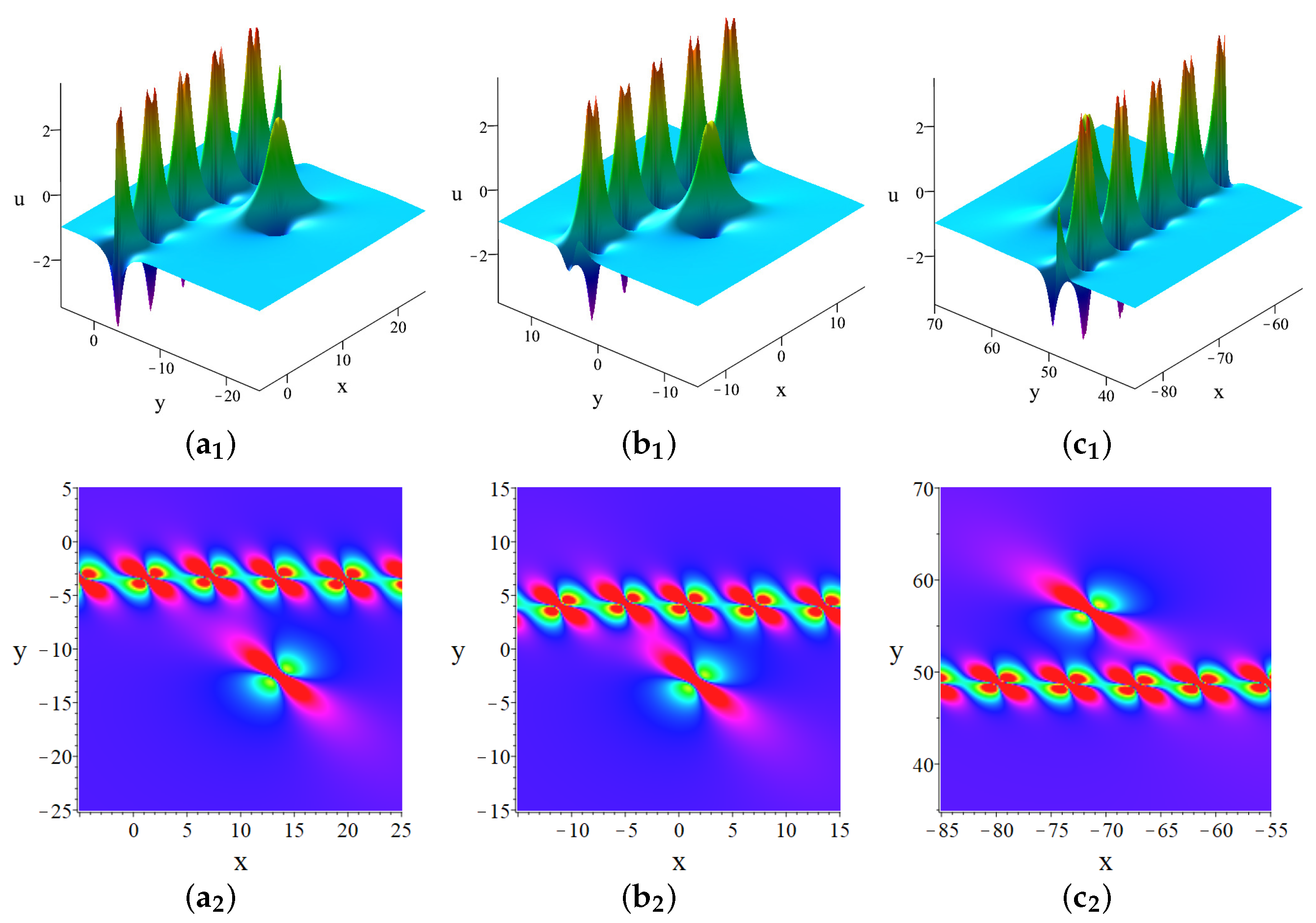
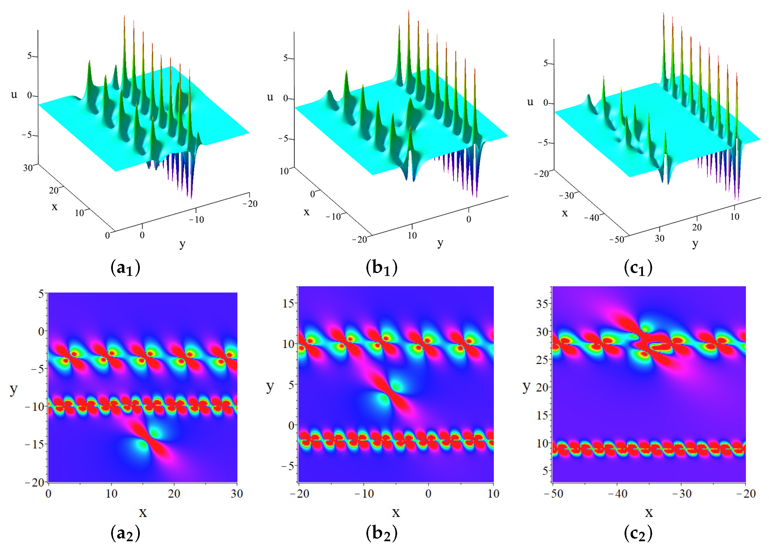
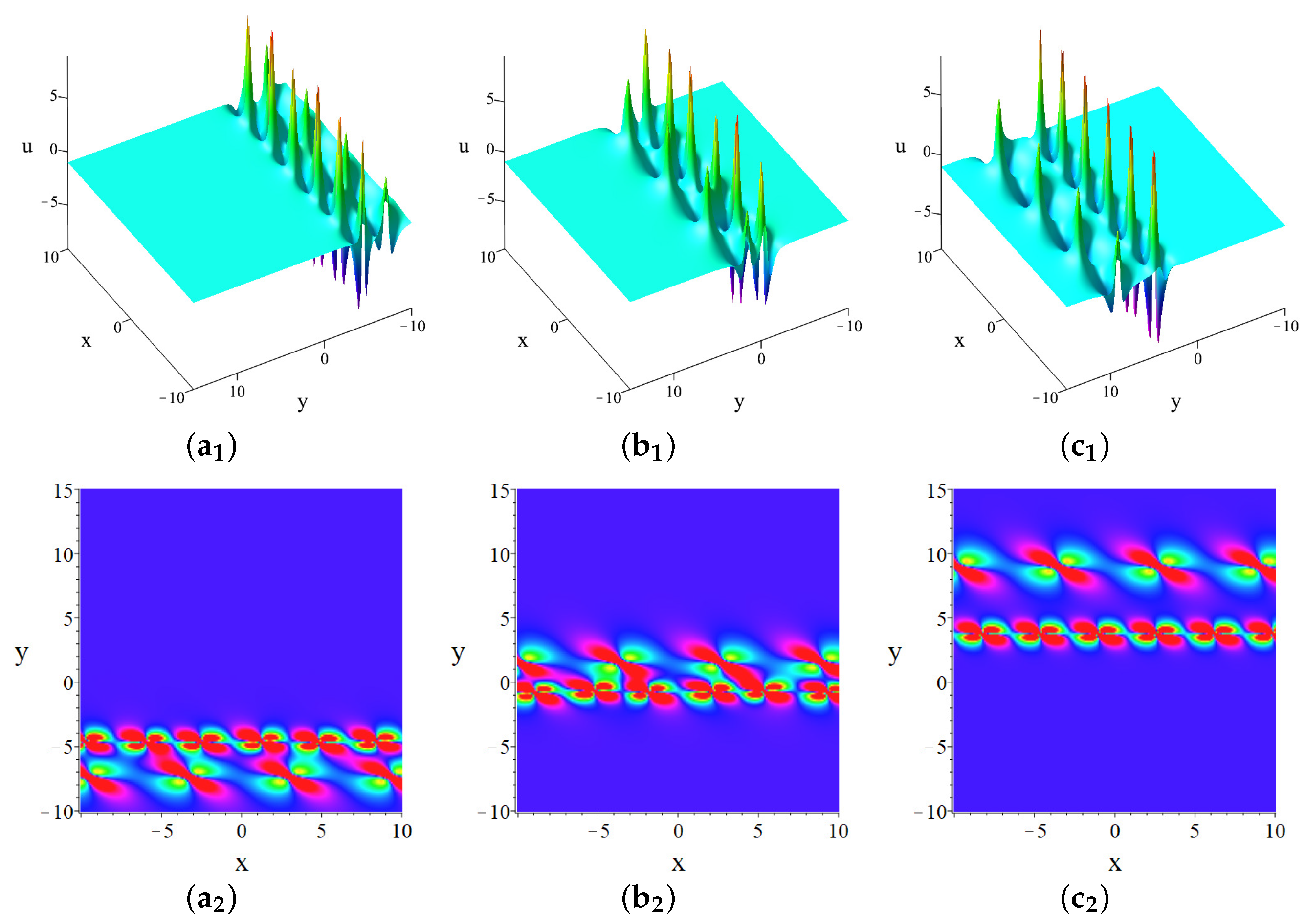
3.2. Breather Solutions

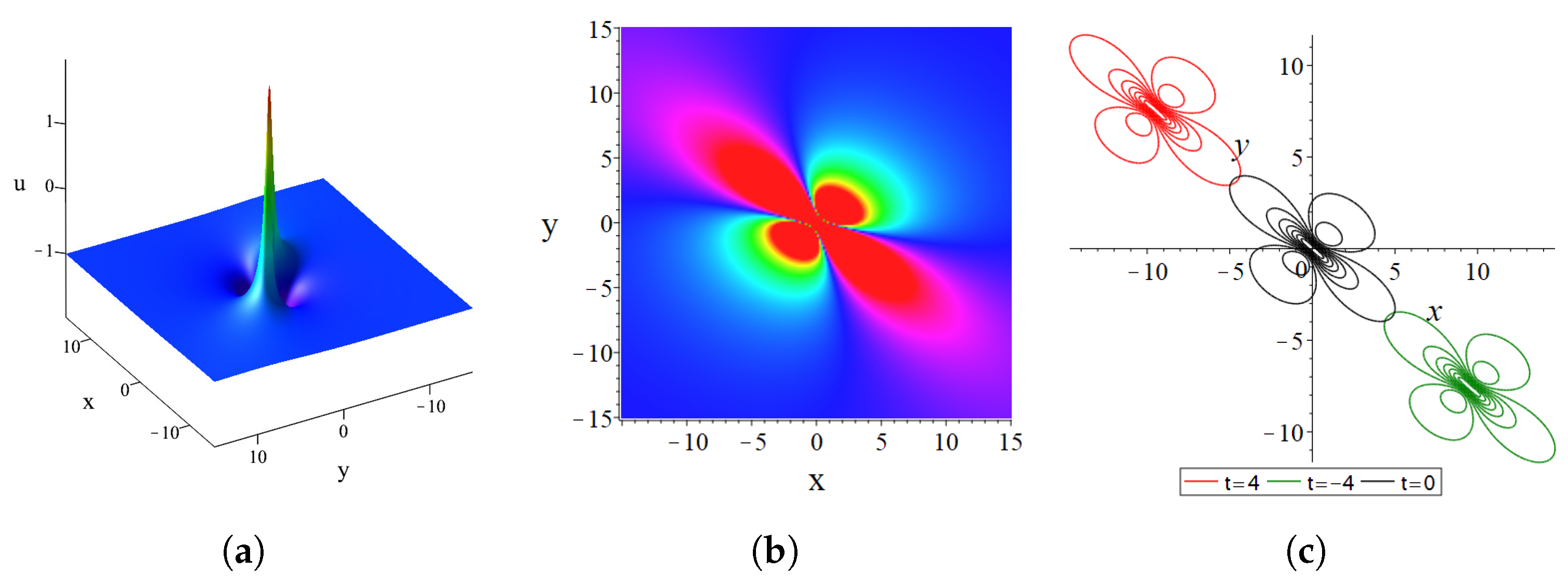
To explore the breather solutions of (1), we select specific functions $G_{ij}^{\left(n\right)}$, $a_i^{\left(n\right)}$ and $b_j^{\left(n\right)}$ as follows:

$$\begin{array}{cc}\hfill & G_{ij}^{\left(n\right)}={\delta }_{ij}+{\displaystyle \frac{1}{{\mu }_i+{\nu }_j}}{a}_i^{\left(n\right)}{b}_j^{\left(n\right)},\hfill \\ \hfill & a_i^{\left(n\right)}={\mu }_i^n({\mu }_i+{\nu }_i){\mathrm{e}}^{{\xi }_i},\hfill \\ \hfill & b_j^{\left(n\right)}={(-\frac{1}{{\nu }_j})}^{\left(n\right)}{\mathrm{e}}^{{\eta }_j},\hfill \end{array}$$

(26)

where

$$\begin{array}{cc}\hfill & {\xi }_i={\mu }_i{x}_1+{\mu }_i^2{x}_2+{\mu }_i^3{x}_3+{\mu }_i^4{x}_4+{\xi }_i^0,\hfill \\ \hfill & {\eta }_j={\nu }_j{x}_1-{\nu }_j^2{x}_2+{\nu }_j^3{x}_3-{\nu }_j^4{x}_4+{\eta }_j^0.\hfill \end{array}$$

(27)

Here, ${\mu }_i$ and ${\nu }_j$ are complex constants, while ${\xi }_i^0$ and ${\eta }_j^0$ are real constants. Additionally, ${\delta }_{ij}=1$ if $i=j$, and it is 0 otherwise. Based on these definitions and (6), we can calculate the determinant as

$$f={\tau }_0=\underset{1⩽i,j⩽N}{det}\left(G_{ij}^{\left(0\right)}\right)={\left|{\delta }_{ij}+{\displaystyle \frac{{\mu }_i+{\nu }_i}{{\mu }_i+{\nu }_j}}{\mathrm{e}}^{{\xi }_i+{\eta }_j}\right|}_{N\times N},$$

(28)

where

$$\begin{array}{cc}\hfill & {\xi }_i=\mathrm{I}{\mu }_{i}x+\mathrm{I}{\mu }_i^{2}y-2\mathrm{I}{\mu }_i^{3}t+{\xi }_i^0,\hfill \\ \hfill & {\eta }_j=\mathrm{I}{\nu }_{j}x-\mathrm{I}{\nu }_j^{2}y-2\mathrm{I}{\nu }_j^{3}t+{\eta }_j^0.\hfill \end{array}$$

(29)

We set $N=2M$ and choose the parameters as follows:

$$\begin{array}{ccccc}\hfill p_{2k-1}=-{\phi }_k+{\displaystyle \frac{{\psi }_k}{2}},& & \hfill p_{2k}=-{\phi }_k^{*}-{\displaystyle \frac{{\psi }_k}{2}},& & \hfill {\xi }_{2k-1}^0={\xi }_{2k}^0={\xi }_k^0,\end{array}$$

(30)

$$\begin{array}{ccccc}\hfill q_{2k-1}={\phi }_k+{\displaystyle \frac{{\psi }_k}{2}},& & \hfill q_{2k}={\phi }_k^{*}-{\displaystyle \frac{{\psi }_k}{2}},& & \hfill {\eta }_{2k-1}^0={\eta }_{2k}^0={\eta }_k^0,\end{array}$$

(31)

where ${\phi }_k$ denotes complex constants; ${\psi }_k$, ${\xi }_k^0$, ${\eta }_k^0$ are real constants; * indicates conjugation; and k takes values from 1 to M. Under these conditions, the breather solution of (1) is given by (16), where $f={\Delta }_0\left|D\right|$, ${\Delta }_0={\mathrm{e}}^{{\sum }_{k=1}^M{\varsigma }_k+{\varsigma }_k^{*}}{\prod }_{k=1}^M{\psi }_k^2$, and D is defined as

$$D_{k,k}=\left(\begin{array}{cc}{\displaystyle \frac{1}{{\psi }_k}}(1+{\mathrm{e}}^{-{\varsigma }_k})& {\displaystyle \frac{1}{{\phi }_k^{*}-{\phi }_k}}\\ {\displaystyle \frac{1}{{\phi }_k^{*}-{\phi }_k}}& {\displaystyle \frac{1}{{\psi }_k}}(1+{\mathrm{e}}^{-{\varsigma }_k^{*}})\end{array}\right),D_{k,l}=\left(\begin{array}{cc}{\displaystyle \frac{1}{-{\phi }_k+{\phi }_l+\frac{{\psi }_k+{\psi }_l}{2}}}& {\displaystyle \frac{1}{-{\phi }_k+{\phi }_l^{*}+\frac{{\psi }_k-{\psi }_l}{2}}}\\ {\displaystyle \frac{1}{{\phi }_k^{*}-{\phi }_l+\frac{{\psi }_k-{\psi }_l}{2}}}& {\displaystyle \frac{1}{{\phi }_k^{*}-{\phi }_l^{*}+\frac{{\psi }_k+{\psi }_l}{2}}}\end{array}\right),$$

(32)

with

$${\varsigma }_k={\psi }_k(\mathrm{I}x-2\mathrm{I}{\phi }_{k}y-{\displaystyle \frac{\mathrm{I}}{2}}(12{\phi }_k^2+{\psi }_k^2)t)+{\varsigma }_k^0,$$

(33)

where ${\psi }_k^2{\phi }_k+4{\phi }_k^3=1$.

When $M=1$, the one-breather solutions of (1) can be expressed as

$$\begin{array}{c}\hfill f={\psi }_1^2{\mathrm{e}}^{{\varsigma }_1+{\varsigma }_1^{*}}\left|\begin{array}{cc}{\displaystyle \frac{1}{{\psi }_1}}(1+{\mathrm{e}}^{-{\varsigma }_1})& {\displaystyle \frac{1}{{\phi }_1^{*}-{\phi }_1}}\\ {\displaystyle \frac{1}{{\phi }_1^{*}-{\phi }_1}}& {\displaystyle \frac{1}{{\psi }_1}}(1+{\mathrm{e}}^{-{\varsigma }_1^{*}})\end{array}\right|=\begin{array}{c}\hfill 1+{\mathrm{e}}^{{\varsigma }_1}+{\mathrm{e}}^{{\varsigma }_1^{*}}+A_{12}{\mathrm{e}}^{{\varsigma }_1+{\varsigma }_1^{*}},\end{array}\end{array}$$

(34)

where

$${\varsigma }_1={\psi }_1(\mathrm{I}x-2\mathrm{I}{\phi }_{1}y-{\displaystyle \frac{\mathrm{I}}{2}}(12{\phi }_1^2+{\psi }_1^2)t)+{\varsigma }_1^0,$$

(35)

$$A_{12}=1-{\displaystyle \frac{{\psi }_1^2}{{({\phi }_1^{*}-{\phi }_1)}^2}}.$$

(36)

Considering ${\phi }_i={\alpha }_i+\mathrm{I}{\beta }_i$, expression (34) can be rephrased as follows:

$$f=1+{\mathrm{e}}^{{\Theta }_1}cos{\Theta }_2+A_{12}{\mathrm{e}}^{2{\Theta }_2},$$

(37)

with

$$\begin{array}{cc}\hfill & {\Theta }_1=2\beta {\psi }_{1}y+12\alpha \beta {\psi }_{1}t+{\varsigma }_1^0,\hfill \\ \hfill & {\Theta }_2={\psi }_{1}x-2\alpha {\psi }_{1}y-6{\psi }_1({\alpha }^2-{\beta }^2)t.\hfill \end{array}$$

(38)

The one-breather solution exhibits localization in the ${\Theta }_1$ direction and periodicity in the ${\Theta }_2$ direction. In Figure 2, the red line represents the characteristic line ${\Theta }_1=0$, while the blue line represents the characteristic line ${\Theta }_2=0$. The solution, defined by ${\phi }_1={\alpha }_1+i{\beta }_1$, is illustrated in Figure 2 and moves along the y-axis over time.

When $M=2$, two-breather solutions of (1) manifest as depicted in Figure 3. These solutions propagate along the y-axis over time, exhibiting distinct velocities. Notably, breathers with larger periods are observed to move faster than those with shorter periods. This behavior highlights the dynamic nature of multi-breathers in the context of the ANNV equation.

For $M=3$, three-breather solutions are obtained, as shown in Figure 4. These solutions further illustrate the complex dynamics and interactions inherent in multi-breather phenomena, providing deeper insights into the underlying nonlinear processes.

3.3. Lump Solutions

To derive the lump solutions for (1), we take the long-wave limit of the breather solutions by setting ${\psi }_k\to 0$ for $k=1,\cdots ,M$, and ${\mathrm{e}}^{{\varsigma }_k^0}=-1$. This leads to the definition ${\vartheta }_k=\underset{{\psi }_k\to 0}{lim}{\displaystyle \frac{1}{{\psi }_k}}(1+{\mathrm{e}}^{-{\varsigma }_k})$. Under these conditions, the M-order lump solution for (1) is given by

$$u=-1+{(2lnf)}_{xy},$$

(39)

where $f=\left|A\right|$ and A is defined by

$$A_{k,k}=\left(\begin{array}{cc}{\vartheta }_k& {\displaystyle \frac{1}{-{\phi }_k+{\phi }_k^{*}}}\\ {\displaystyle \frac{1}{-{\phi }_k+{\phi }_k^{*}}}& {\vartheta }_k^{*}\end{array}\right),A_{k,l}=\left(\begin{array}{cc}{\displaystyle \frac{1}{-{\phi }_k+{\phi }_l}}& {\displaystyle \frac{1}{-{\phi }_k+{\phi }_l^{*}}}\\ {\displaystyle \frac{1}{{\phi }_k^{*}{\phi }_l}}& {\displaystyle \frac{1}{{\phi }_k^{*}-{\phi }_l^{*}}}\end{array}\right),$$

(40)

with

$${\vartheta }_k=\mathrm{I}x-2\mathrm{I}{\phi }_{k}y-6\mathrm{I}{\phi }_k^{2}t,$$

(41)

where ${\Phi }_k$$(k=1,2,\dots ,M)$ denotes complex constants satisfying the condition $4{\phi }_k^3+{\phi }_k{\psi }_k^2=1$. This approach allows us to obtain M-order lump solutions u for (1), highlighting the rich dynamical behavior of these localized wave structures.

When $M=1$, the first-order lump solutions of (1) can be expressed as

$$\begin{array}{c}\hfill f=\left|\begin{array}{cc}{\vartheta }_1& {\displaystyle \frac{1}{-{\phi }_1+{\phi }_1^{*}}}\\ {\displaystyle \frac{1}{-{\phi }_1+{\phi }_1^{*}}}& {\vartheta }_1^{*}\end{array}\right|=\begin{array}{c}\hfill {\vartheta }_1{\vartheta }_1^{*}-{\displaystyle \frac{1}{{({\phi }_1^{*}-{\phi }_1)}^2}},\end{array}\end{array}$$

(42)

where

$${\vartheta }_1=\mathrm{I}x-2\mathrm{I}{\phi }_{1}y-6\mathrm{I}{\phi }_1^{2}t.$$

(43)

Figure 5 presents the plots of the first-order lump solution. The left (Figure 5a) panel shows the three-dimensional visualization, the middle panel (Figure 5b) displays the density map, and the right panel (Figure 5c) illustrates the temporal evolution. These visualizations provide insights into the spatial and temporal characteristics of the lump solution. Here, ${\phi }_1={\alpha }_1+\mathrm{I}{\beta }_1$, where ${\alpha }_1$ and ${\beta }_1$ are the real and imaginary parts, respectively. To avoid singularities, the real part ${\alpha }_1$ must be non-zero. For a fixed time t, as $(x,y)\to \infty$, the lump solution $u=-1$, indicating that the lump propagates on a constant background. At $t=0$, the critical points of the first-order lump solution are obtained by solving ${\displaystyle \frac{\partial u}{\partial x}}=0$ and ${\displaystyle \frac{\partial u}{\partial y}}=0$. The results are as follows: maximum peak amplitude $u=2$ at the point $(x,y)=(0,0)$ and minimum peak amplitude $u=-2$ at the points $(x,y)=(\pm {\displaystyle \frac{2·2^{1/6}}{6}},\pm \frac{2^{5/6}}{3})$. However, due to the reduction condition, the ANNV Equation (1) supports only a first-order lump solution.

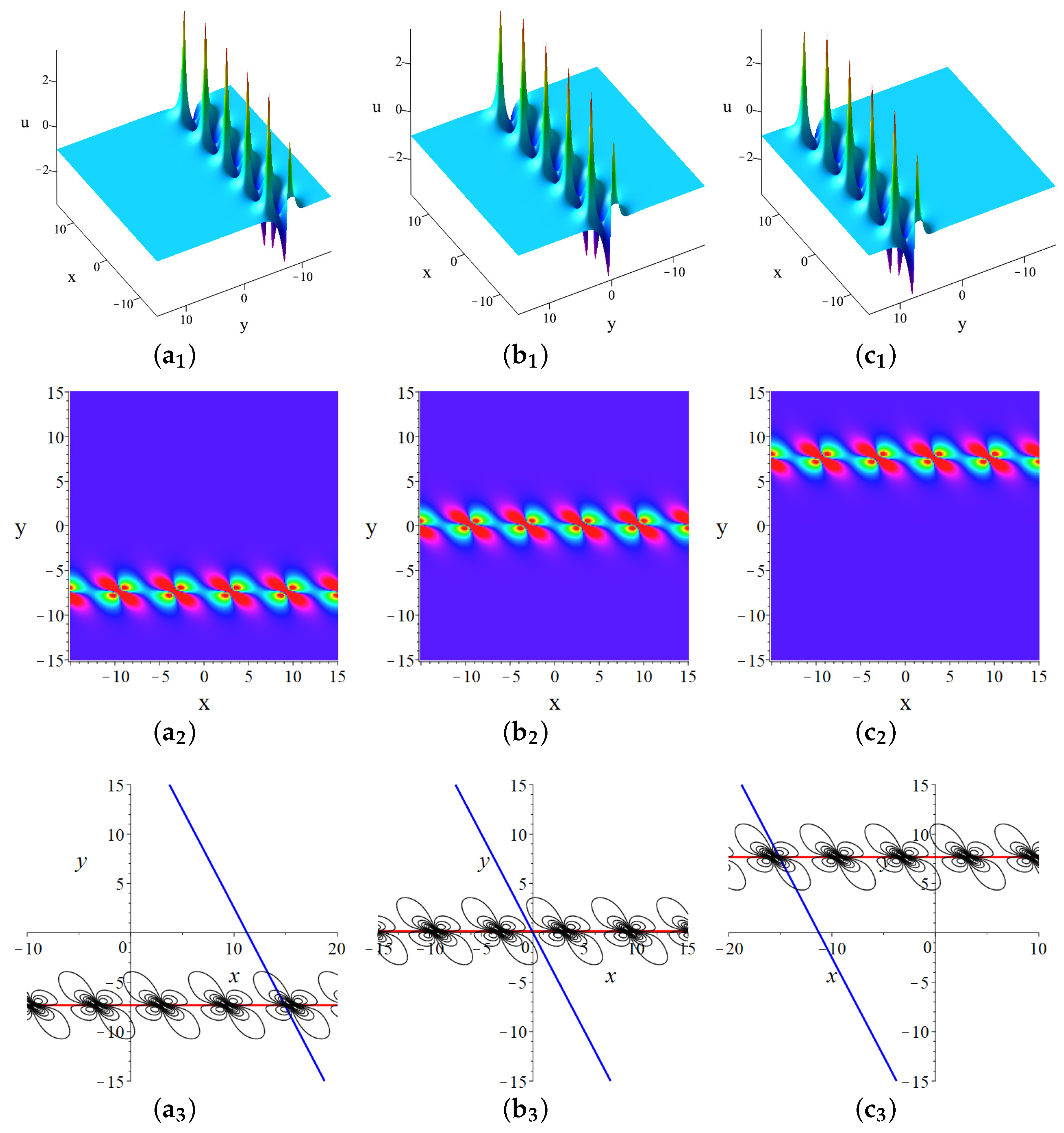
3.4. Hybrid Solutions

To derive hybrid solutions for the ANNV Equation (1), we consider the long-wave limit of the breather solutions. Specifically, we define $N=M+M^{\prime }$ and take ${\varpi }_k\to 0$ for $k=1,\cdots ,M$, while also setting the phase parameter ${\mathrm{e}}^{{\varsigma }_k^0}=-1$.

Under these conditions, the hybrid solutions combining M-order lump with $M^{\prime }$-breather for (1) are given by (16), where

$$f=\left|\begin{array}{cc}A& B\\ C& D\end{array}\right|,$$

(44)

with A, B, C, and D defined as follows: A is a $2M\times 2M$ matrix given as

$$A_{k,k}=\left(\begin{array}{cc}{\vartheta }_k& {\displaystyle \frac{1}{-{\phi }_k+{\phi }_k^{*}}}\\ {\displaystyle \frac{1}{-{\phi }_k+{\phi }_k^{*}}}& {\vartheta }_k^{*}\end{array}\right),A_{k,l}=\left(\begin{array}{cc}{\displaystyle \frac{1}{-{\phi }_k+{\phi }_l}}& {\displaystyle \frac{1}{-{\phi }_k+{\phi }_l^{*}}}\\ {\displaystyle \frac{1}{{\phi }_k^{*}-{\phi }_l}}& {\displaystyle \frac{1}{{\phi }_k^{*}-{\phi }_l^{*}}}\end{array}\right),$$

(45)

B is a $2M\times 2M^{\prime }$ matrix given as

$$B_{k,l}=\left(\begin{array}{cc}{\displaystyle \frac{1}{-{\phi }_k+{\phi }_l+\frac{{\psi }_l}{2}}}& {\displaystyle \frac{1}{-{\phi }_k+{\phi }_l^{*}-\frac{{\psi }_l}{2}}}\\ {\displaystyle \frac{1}{{\phi }_k^{*}-{\phi }_l-\frac{{\psi }_l}{2}}}& {\displaystyle \frac{1}{{\phi }_k^{*}-{\phi }_l^{*}+\frac{{\psi }_l}{2}}}\end{array}\right),$$

(46)

C is a $2M^{\prime }\times 2M$ matrix given as

$$C_{k,l}=\left(\begin{array}{cc}{\displaystyle \frac{1}{-{\phi }_k+{\phi }_l+\frac{{\psi }_k}{2}}}& {\displaystyle \frac{1}{-{\phi }_k+{\phi }_l^{*}+\frac{{\psi }_k}{2}}}\\ {\displaystyle \frac{1}{{\phi }_k^{*}-{\phi }_l+\frac{{\psi }_k}{2}}}& {\displaystyle \frac{1}{{\phi }_k^{*}-{\phi }_l^{*}+\frac{{\psi }_k}{2}}}\end{array}\right),$$

(47)

and D is a $2M^{\prime }\times 2M^{\prime }$ matrix given as

$$D_{k,k}=\left(\begin{array}{cc}{\displaystyle \frac{1}{{\psi }_k}}(1+{\mathrm{e}}^{-{\varsigma }_k})& {\displaystyle \frac{1}{-{\phi }_k+{\phi }_k^{*}}}\\ {\displaystyle \frac{1}{-{\phi }_k+{\phi }_k^{*}}}& {\displaystyle \frac{1}{{\psi }_k}}(1+{\mathrm{e}}^{-{\varsigma }_k^{*}})\end{array}\right),D_{k,l}=\left(\begin{array}{cc}{\displaystyle \frac{1}{-{\phi }_k+{\phi }_l+\frac{{\psi }_k+{\psi }_l}{2}}}& {\displaystyle \frac{1}{-{\phi }_k+{\phi }_l^{*}+\frac{{\psi }_k-{\psi }_l}{2}}}\\ {\displaystyle \frac{1}{{\phi }_k^{*}-{\phi }_l+\frac{{\psi }_k-{\psi }_l}{2}}}& {\displaystyle \frac{1}{{\phi }_k^{*}-{\phi }_l^{*}+\frac{{\psi }_k+{\psi }_l}{2}}}\end{array}\right),$$

(48)

with

$$\begin{array}{cc}& {\varsigma }_k={\psi }_k(\mathrm{I}x-2\mathrm{I}{\phi }_{k}y-{\displaystyle \frac{\mathrm{I}}{2}}(12{\phi }_k^2+{\psi }_k^2)t)+{\varsigma }_k^0,\end{array}$$

(49)

$$\begin{array}{cc}& {\vartheta }_k=\mathrm{I}x-2\mathrm{I}{\phi }_{k}y-6\mathrm{I}{\phi }_k^{2}t,\end{array}$$

(50)

where M and $M^{\prime }$ denote positive integers, and ${\phi }_k$ is a complex constant. The condition $4{\phi }_k^3+{\phi }_k{\psi }_k^2=1$ must be satisfied.

The hybrid solutions of (1) combine lump and breather solutions, showcasing the rich dynamical behavior of these nonlinear wave structures. Specific cases are detailed below.

• When $M=1$ and $M^{\prime }=1$, the first-order lump and one-breather hybrid solution is given by the determinant

  $$f=\left|\begin{array}{cccc}{\vartheta }_1& {\displaystyle \frac{1}{-{\phi }_1+{\phi }_1^{*}}}& {\displaystyle \frac{1}{-{\phi }_1+{\phi }_2+\frac{{\psi }_2}{2}}}& {\displaystyle \frac{1}{-{\phi }_1+{\phi }_2^{*}-\frac{{\psi }_2}{2}}}\\ {\displaystyle \frac{1}{-{\phi }_1+{\phi }_1^{*}}}& {\vartheta }_1^{*}& {\displaystyle \frac{1}{{\phi }_1^{*}-{\phi }_2-\frac{{\psi }_2}{2}}}& {\displaystyle \frac{1}{{\phi }_1^{*}-{\phi }_2^{*}+\frac{{\psi }_2}{2}}}\\ {\displaystyle \frac{1}{-{\phi }_2+{\phi }_1+\frac{{\psi }_2}{2}}}& {\displaystyle \frac{1}{-{\phi }_2+{\phi }_1^{*}+\frac{{\psi }_2}{2}}}& {\displaystyle \frac{1}{{\psi }_2}}(1+{\mathrm{e}}^{-{\varsigma }_2})& {\displaystyle \frac{1}{{\phi }_2^{*}-{\phi }_2}}\\ {\displaystyle \frac{1}{{\phi }_2^{*}-{\phi }_1+\frac{{\psi }_2}{2}}}& {\displaystyle \frac{1}{{\phi }_2^{*}-{\phi }_1^{*}+\frac{{\psi }_2}{2}}}& {\displaystyle \frac{1}{{\phi }_2^{*}-{\phi }_2}}& {\displaystyle \frac{1}{{\psi }_2}}(1+{\mathrm{e}}^{-{\varsigma }_2^{*}})\end{array}\right|,$$

  (51)

  as depicted in Figure 6.
• When $M=1$ and $M^{\prime }=2$, the first-order lump and two-breather hybrid solution is given by the determinant

  $$f=\left|\begin{array}{cccccc}{\vartheta }_1& {\displaystyle \frac{1}{-{\phi }_1+{\phi }_1^{*}}}& {\displaystyle \frac{1}{-{\phi }_1+{\phi }_2+\frac{{\psi }_2}{2}}}& {\displaystyle \frac{1}{-{\phi }_1+{\phi }_2^{*}-\frac{{\psi }_2}{2}}}& {\displaystyle \frac{1}{-{\phi }_1+{\Phi }_3+\frac{{\psi }_3}{2}}}& {\displaystyle \frac{1}{-{\phi }_1+{\Phi }_3^{*}-\frac{{\psi }_3}{2}}}\\ {\displaystyle \frac{1}{-{\phi }_1+{\phi }_1^{*}}}& {\vartheta }_1^{*}& {\displaystyle \frac{1}{{\phi }_1^{*}-{\phi }_2-\frac{{\psi }_2}{2}}}& {\displaystyle \frac{1}{{\phi }_1^{*}-{\phi }_2^{*}+\frac{{\psi }_2}{2}}}& {\displaystyle \frac{1}{{\phi }_1^{*}-{\Phi }_3-\frac{{\psi }_3}{2}}}& {\displaystyle \frac{1}{{\phi }_1^{*}-{\Phi }_3^{*}+\frac{{\psi }_3}{2}}}\\ {\displaystyle \frac{1}{-{\phi }_2+{\phi }_1+\frac{{\psi }_2}{2}}}& {\displaystyle \frac{1}{-{\phi }_2+{\phi }_1^{*}+\frac{{\psi }_2}{2}}}& {\displaystyle \frac{1}{{\psi }_2}}(1+{\mathrm{e}}^{-{\varsigma }_2})& {\displaystyle \frac{1}{{\phi }_2^{*}-{\phi }_2}}& {\displaystyle \frac{1}{-{\phi }_2+{\Phi }_3+\frac{{\psi }_2}{2}}}& {\displaystyle \frac{1}{-{\phi }_2+{\Phi }_3^{*}+\frac{{\psi }_2}{2}}}\\ {\displaystyle \frac{1}{{\phi }_2^{*}-{\phi }_1+\frac{{\psi }_2}{2}}}& {\displaystyle \frac{1}{{\phi }_2^{*}-{\phi }_1^{*}+\frac{{\psi }_2}{2}}}& {\displaystyle \frac{1}{{\phi }_2^{*}-{\phi }_2}}& {\displaystyle \frac{1}{{\psi }_2}}(1+{\mathrm{e}}^{-{\varsigma }_2^{*}})& {\displaystyle \frac{1}{{\phi }_2^{*}-{\Phi }_3+\frac{{\psi }_2}{2}}}& {\displaystyle \frac{1}{{\phi }_2^{*}-{\Phi }_3^{*}+\frac{{\psi }_2}{2}}}\\ {\displaystyle \frac{1}{-{\Phi }_3+{\phi }_1+\frac{{\psi }_3}{2}}}& {\displaystyle \frac{1}{-{\Phi }_3+{\phi }_1^{*}+\frac{{\psi }_3}{2}}}& {\displaystyle \frac{1}{-{\Phi }_3+{\phi }_2+\frac{{\psi }_3}{2}}}& {\displaystyle \frac{1}{-{\Phi }_3+{\phi }_2^{*}+\frac{{\psi }_3}{2}}}& {\displaystyle \frac{1}{{\psi }_3}}(1+{\mathrm{e}}^{-{\varsigma }_3})& {\displaystyle \frac{1}{{\Phi }_3^{*}-{\Phi }_3}}\\ {\displaystyle \frac{1}{{\Phi }_3^{*}-{\phi }_1+\frac{{\psi }_3}{2}}}& {\displaystyle \frac{1}{{\Phi }_3^{*}-{\phi }_1^{*}+\frac{{\psi }_3}{2}}}& {\displaystyle \frac{1}{{\Phi }_3^{*}-{\phi }_2+\frac{{\psi }_3}{2}}}& {\displaystyle \frac{1}{{\Phi }_3^{*}-{\phi }_2^{*}+\frac{{\psi }_3}{2}}}& {\displaystyle \frac{1}{{\Phi }_3^{*}-{\Phi }_3}}& {\displaystyle \frac{1}{{\psi }_3}}(1+{\mathrm{e}}^{-{\varsigma }_3^{*}})\end{array}\right|,$$

  (52)

  as depicted in Figure 7.

As depicted in Figure 6 and Figure 7, both the breather and lump components of the hybrid solutions propagate along the negative x-axis and the positive y-axis. The lump component moves faster than the breather component. In Figure 7, the two-breather case exhibits distinct periods, with the breather having a larger period moving faster than the one with a smaller period. This highlights the intricate interactions between lump and breather solutions in the context of (1).

Figure 6. The hybrid solution combining a first-order lump with one breather at (${\mathbf{a}}_{\mathbf{1}}$,${\mathbf{a}}_{\mathbf{2}}$) $t=-3$, (${\mathbf{b}}_{\mathbf{1}}$,${\mathbf{b}}_{\mathbf{2}}$) $t=0$, (${\mathbf{c}}_{\mathbf{1}}$,${\mathbf{c}}_{\mathbf{2}}$) $t=30$. The parameters are ${\phi }_1=-{\displaystyle \frac{2^{\frac{1}{3}}}{4}}+{\displaystyle \frac{2^{\frac{1}{3}}\sqrt{3}}{4}}\mathrm{I},{\psi }_2=1$.

Figure 6. The hybrid solution combining a first-order lump with one breather at (${\mathbf{a}}_{\mathbf{1}}$,${\mathbf{a}}_{\mathbf{2}}$) $t=-3$, (${\mathbf{b}}_{\mathbf{1}}$,${\mathbf{b}}_{\mathbf{2}}$) $t=0$, (${\mathbf{c}}_{\mathbf{1}}$,${\mathbf{c}}_{\mathbf{2}}$) $t=30$. The parameters are ${\phi }_1=-{\displaystyle \frac{2^{\frac{1}{3}}}{4}}+{\displaystyle \frac{2^{\frac{1}{3}}\sqrt{3}}{4}}\mathrm{I},{\psi }_2=1$.

Figure 7. The hybrid solution combining a first-order lump with two breathers at (${\mathbf{a}}_{\mathbf{1}}$,${\mathbf{a}}_{\mathbf{2}}$) $t=-6$; (${\mathbf{b}}_{\mathbf{1}}$,${\mathbf{b}}_{\mathbf{2}}$) $t=3$; (${\mathbf{c}}_{\mathbf{1}}$,${\mathbf{c}}_{\mathbf{2}}$) $t=15$. The parameters are ${\phi }_1=-{\displaystyle \frac{2^{\frac{1}{3}}}{4}}+{\displaystyle \frac{2^{\frac{1}{3}}\sqrt{3}}{4}}\mathrm{I},{\psi }_2=1,{\psi }_3=\sqrt{3}$.

Figure 7. The hybrid solution combining a first-order lump with two breathers at (${\mathbf{a}}_{\mathbf{1}}$,${\mathbf{a}}_{\mathbf{2}}$) $t=-6$; (${\mathbf{b}}_{\mathbf{1}}$,${\mathbf{b}}_{\mathbf{2}}$) $t=3$; (${\mathbf{c}}_{\mathbf{1}}$,${\mathbf{c}}_{\mathbf{2}}$) $t=15$. The parameters are ${\phi }_1=-{\displaystyle \frac{2^{\frac{1}{3}}}{4}}+{\displaystyle \frac{2^{\frac{1}{3}}\sqrt{3}}{4}}\mathrm{I},{\psi }_2=1,{\psi }_3=\sqrt{3}$.

In addition to the hybrid solutions discussed earlier, we have discovered a novel solution structure that represents the interaction between a lump solution and a soliton solution. The derivation process is as follows. First, we rewrite (3) as

$$\begin{array}{cc}\hfill & 2\left({\displaystyle \frac{{\partial }^{2}f}{\partial t\partial y}}\right)f-2\left({\displaystyle \frac{\partial f}{\partial t}}\right)\left({\displaystyle \frac{\partial f}{\partial y}}\right)+2\left({\displaystyle \frac{{\partial }^{4}f}{\partial x^3\partial y}}\right)f-2\left({\displaystyle \frac{{\partial }^{3}f}{\partial x^3}}\right)\left({\displaystyle \frac{\partial f}{\partial y}}\right)\hfill \\ \hfill & -6\left({\displaystyle \frac{{\partial }^{3}f}{\partial x^2\partial y}}\right)\left({\displaystyle \frac{\partial f}{\partial x}}\right)+6\left({\displaystyle \frac{{\partial }^{2}f}{\partial x^2}}\right)\left({\displaystyle \frac{{\partial }^{2}f}{\partial x\partial y}}\right)-6\left({\displaystyle \frac{{\partial }^{2}f}{\partial x^2}}\right)f+6{\left({\displaystyle \frac{\partial f}{\partial x}}\right)}^2=0.\hfill \end{array}$$

(53)

To construct a hybrid solution that includes both lump and line soliton solutions, we assume the following form for the solution:

$$f={(k_{1}x+p_{1}y+t{\epsilon }_1+{\eta }_1)}^2+{(k_{2}x+p_{2}y+t{\epsilon }_2+{\eta }_2)}^2+a{\mathrm{e}}^{(k_{3}x+p_{3}y+t{\epsilon }_3)}+\eta ,$$

(54)

where the quadratic function represents a lump, and the exponential function represents a soliton. By substituting the above expression of f into (53) and collecting the coefficients of x, y, t, and ${\mathrm{e}}^{(k_{3}x+p_{3}y+t{\epsilon }_3)}$, we solve the resulting polynomial system to obtain three sets of representative parameters. The first set:

$$\begin{array}{cc}\hfill a& =0,k_1=k_1,k_2=k_2,k_3=k_3,p_1=p_1,\hfill \\ \hfill p_2& =p_2,p_3=p_3,{\epsilon }_3={\epsilon }_3,{\eta }_1={\eta }_1,{\eta }_2={\eta }_2,\hfill \\ \hfill {\epsilon }_1& ={\displaystyle \frac{3(k_1^2{p}_1+2k_1{k}_2{p}_2-k_2^2{p}_1)}{p_1^2+p_2^2}},{\epsilon }_2=-{\displaystyle \frac{3(k_1^2{p}_2-2k_1{k}_2{p}_1-k_2^2{p}_2)}{p_1^2+p_2^2}},\hfill \\ \hfill \eta & ={\displaystyle \frac{k_1^3{p}_1^3+k_1^3{p}_1{p}_2^2+k_1^2{k}_2{p}_1^2{p}_2+k_1^2{k}_2{p}_2^3+k_1{k}_2^2{p}_1^3+k_1{k}_2^2{p}_1{p}_2^2+k_2^3{p}_1^2{p}_2+k_2^3{p}_2^3}{{(k_1{p}_2-k_2{p}_1)}^2}}.\hfill \end{array}$$

(55)

The second set:

$$\begin{array}{cc}\hfill a& =a,\eta ={\displaystyle \frac{(-k_3^4{p}_2^2+4k_1^2)(k_3^8{p}_2^4+8k_1^2{k}_3^4{p}_2^2+16k_1^4)}{64k_3^6{p}_2^2{k}_1^2}},{\eta }_1={\eta }_1,{\eta }_2={\eta }_2,\hfill \\ \hfill k_1& =k_1,k_2={\displaystyle \frac{-k_3^4{p}_2^2+4k_1^2}{4k_3^2{p}_2}},k_3=k_3,p_1=0,p_2=p_2,p_3={\displaystyle \frac{4k_3^3{p}_2^2}{k_3^4{p}_2^2+4k_1^2}},\hfill \\ \hfill {\epsilon }_1& ={\displaystyle \frac{3k_1(-k_3^4{p}_2^2+4k_1^2)}{2k_3^2{p}_2^2}},{\epsilon }_2={\displaystyle \frac{3(k_3^8{p}_2^4-24k_1^2{k}_3^4{p}_2^2+16k_1^4)}{16k_3^4{p}_2^3}},{\epsilon }_3={\displaystyle \frac{-k_3^4{p}_2^2+12k_1^2}{4k_3{p}_2^2}}.\hfill \end{array}$$

(56)

The third set:

$$\begin{array}{cc}\hfill a& =a,\eta =0,{\eta }_1={\eta }_1,{\eta }_2={\eta }_2,k_1={\displaystyle \frac{1}{2}}{k}_3^2{p}_2,k_2=-{\displaystyle \frac{1}{2}}{k}_3^2{p}_1,k_3=k_3,\hfill \\ \hfill p_1& =p_1,p_2=p_2,p_3={\displaystyle \frac{2}{k_3}},{\epsilon }_1=-{\displaystyle \frac{3k_3^4{p}_1}{4}},{\epsilon }_2=-{\displaystyle \frac{3k_3^4{p}_2}{4}},{\epsilon }_3={\displaystyle \frac{1}{2}}{k}_3^3.\hfill \end{array}$$

(57)

In the first set of parameters, $a=0$, which implies that the line soliton solution does not exist, and only a lump solution can be obtained. The second and third sets of parameters both allow for an interaction solution between one lump and one soliton. For further analysis, we select the second set of parameters, resulting in

$$\begin{array}{cc}\hfill f& =a{\mathrm{e}}^{\left(k_{3}x+{\displaystyle \frac{4k_3^3{p}_2^{2}y}{k_3^4{p}_2^2+4k_1^2}}+t·{\displaystyle \frac{-k_3^4{p}_2^2+12k_1^2}{4k_3{p}_2^2}}\right)}\hfill \\ \hfill & +{\left(k_{1}x+{\displaystyle \frac{3t{k}_1(-k_3^4{p}_2^2+4k_1^2)}{2k_3^2{p}_2^2}}+{\eta }_1\right)}^2\hfill \\ \hfill & +{\left({\displaystyle \frac{(-k_3^4{p}_2^2+4k_1^2)x}{4k_3^2{p}_2}}+p_{2}y+{\displaystyle \frac{3t(k_3^8{p}_2^4-24k_1^2{k}_3^4{p}_2^2+16k_1^4)}{16k_3^4{p}_2^3}}+{\eta }_2\right)}^2\hfill \\ \hfill & +{\displaystyle \frac{(-k_3^4{p}_2^2+4k_1^2)(k_3^8{p}_2^4+8k_1^2{k}_3^4{p}_2^2+16k_1^4)}{64k_3^6{p}_2^2{k}_1^2}}.\hfill \end{array}$$

(58)

By assigning specific values to the unknown parameters $a=1$, $k_1=1$, $k_3=1$, $p_2=1$, ${\eta }_1=5$, ${\eta }_2=5$, and substituting them into $u=-1+2{(lnf)}_{xx}$, we obtain the interaction solution:

$$\begin{array}{cc}\hfill u=& -1+{\displaystyle \frac{2\left(4·exp\left(x+\frac{4y}{5}+\frac{11t}{4}\right)·\frac{1}{5}+\frac{3}{2}\right)}{exp\left(x+\frac{4y}{5}+\frac{11t}{4}\right)+{\left(x+\frac{9t}{2}+5\right)}^2+{\left(\frac{3x}{4}+y-\frac{21t}{16}+5\right)}^2+\frac{75}{64}}}\hfill \\ \hfill & -{\displaystyle \frac{2\left(exp\left(x+\frac{4y}{5}+\frac{11t}{4}\right)+\frac{25x}{8}+\frac{225t}{32}+\frac{35}{2}+\frac{3y}{2}\right)\left(4·exp\left(x+\frac{4y}{5}+\frac{11t}{4}\right)·\frac{1}{5}+\frac{3x}{2}+2y-\frac{21t}{8}+10\right)}{{\left(exp\left(x+\frac{4y}{5}+\frac{11t}{4}\right)+{\left(x+\frac{9t}{2}+5\right)}^2+{\left(\frac{3x}{4}+y-\frac{21t}{16}+5\right)}^2+\frac{75}{64}\right)}^2}}.\hfill \end{array}$$

(59)

The resulting solution is depicted in Figure 8. Figure 8a shows the three-dimensional visualization, Figure 8b displays the density map.

4. Modulation Stability Analysis

Modulational instability is one of the key mechanisms for the formation of rogue waves. When a wave train is in a state of modulational instability, small perturbations grow over time, causing energy to concentrate in certain specific wave bands from the background wave. This energy concentration can lead to a dramatic increase in the amplitude of local waves, thereby forming rogue waves. For example, the modulational instability solutions of the NLS equation have been extensively studied, and the results show that modulational instability can lead to the formation of rogue waves [44].

To better understand the potential for rogue wave formation within the framework of the ANNV Equation (1), we conduct a modulation stability analysis. We start by reformulating the ANNV Equation (1) as follows:

$$\left\{\begin{array}{c}{u}_t+u_{xxx}+3{\left(uv\right)}_x=0,\hfill \\ u_x=v_y,\hfill \end{array}\right.$$

(60)

where u and v are functions of x, y and t. This system admits constant solutions $u=\alpha$ and $v=\beta$, where $\alpha$ and $\beta$ are arbitrary real numbers. To investigate the stability of these constant solutions, we introduce small perturbations:

$$\left\{\begin{array}{c}u(x,y,t)=\alpha +\delta U(x,y,t),\hfill \\ v(x,y,t)=\beta +\delta V(x,y,t),\hfill \end{array}\right.$$

(61)

where $\delta$ is an infinitesimal parameter representing the amplitude of the perturbations. Substituting these perturbed states into the reformulated ANNV Equation (60) and retaining terms linear in $\delta$, we obtain the linearized system

$$\left\{\begin{array}{c}{U}_t+U_{xxx}+3\left[\alpha V_x+\beta U_x\right]=0,\hfill \\ U_x=V_y.\hfill \end{array}\right.$$

(62)

Next, we assume that the perturbations take the form

$$\left\{\begin{array}{c}U=F{\mathrm{e}}^{gt+iwx+iay},\hfill \\ V=G{\mathrm{e}}^{gt+iwx+iay},\hfill \end{array}\right.$$

(63)

where g, w, and a are constants representing the growth rate, wave number, and transverse wave number, respectively. Substituting these forms into the linearized system yields the following equations:

$$\left\{\begin{array}{c}(g-i{w}^3+3i\beta w)F+3i\alpha wG=0,\hfill \\ iwF=iaG.\hfill \end{array}\right.$$

(64)

From the second equation, we have $G={\displaystyle \frac{w}{a}}F$. Substituting G into the first equation yields the dispersion relation

$$g={\displaystyle \frac{i{w}^2(aw-3\alpha )}{a}}-3i\beta w.$$

(65)

Given that w, a, $\alpha$ and $\beta$ are real numbers, the imaginary part of g must vanish for the system to be stable. This implies that the perturbations do not grow exponentially, indicating that the system is modulationally stable. Consequently, the ANNV Equation (1) does not support rogue wave solutions under these conditions. This analysis highlights the inherent stability of the ANNV equation against small perturbations, shedding light on the absence of rogue wave phenomena in this context.

However, it is important to note that modulational stability does not necessarily exclude the existence of rogue waves in all cases. The formation of rogue waves may also be influenced by other factors, such as higher-order nonlinear effects, initial conditions, and boundary conditions. Therefore, although our analysis indicates that the ANNV equation does not support rogue waves under the current conditions, further research on these additional factors is needed to completely rule out the possibility of rogue wave formation under other conditions.

5. Conclusions

This study consisted of a comprehensive investigation of the ANNV Equation (1) using the KP hierarchy reduction method. By establishing appropriate constraint conditions, we successfully transformed specific equations from the KP hierarchy into (3). This transformation enables the derivation of Gram determinant solutions and facilitates the exploration of various localized wave solutions, including solitons, breathers, lumps, and their hybrid forms. Additionally, through a modulation stability analysis, we determined that the ANNV equation does not support rogue wave solutions. Overall, the findings of this study significantly enhance our understanding of the dynamics and properties of the ANNV Equation (1), filling the gap in the application of the KPRHM to (1). By revealing the rich behaviors of solitons, breathers, lumps, and their hybrid forms, this research contributes to the broader field of nonlinear wave theory. Despite these achievements, we recognize certain limitations. First, not all bilinear forms of integrable equations can be directly linked to the KP equation family, limiting the application of the KP hierarchy reduction method to some specific equations. Second, while exact solutions were obtained through symbolic computation and analytical methods, this study lacked numerical simulations, which could provide more intuitive insights into complex nonlinear phenomena such as soliton collisions and wave stability. Future work will focus on strengthening the numerical simulation component to address these limitations and further expand the depth and breadth of the research.

References

1. Ablowitz, M.J.; Clarkson, P.A. Solitons, Nonlinear Evolution Equations and Inverse Scattering; Cambridge University Press: Cambridge, UK, 1991. [Google Scholar]
2. Zhang, X.; Chen, Y.; Zhang, Y. Breather, lump and X soliton solutions to nonlocal KP equation. Comput. Math. Appl. 2017, 74, 2341–2347. [Google Scholar] [CrossRef]
3. Johnson, R.S. On solutions of the Camassa-Holm equation. Proc. R. Soc. Lond. A 2003, 459, 1687–1708. [Google Scholar] [CrossRef]
4. Kenig, C.E.; Ponce, G.; Vega, L. On the generalized Benjamin-Ono equation. Trans. Am. Math. Soc. 1994, 342, 155–172. [Google Scholar] [CrossRef]
5. Zhou, Z.; Ma, W.X.; Zhou, R. Finite-dimensional integrable systems associated with the Davey-Stewartson I equation. Nonlinearity 2001, 14, 701. [Google Scholar]
6. Ablowitz, M.J.; Musslimani, Z.H. Inverse scattering transform for the integrable nonlocal nonlinear Schrödinger equation. Nonlinearity 2016, 29, 915. [Google Scholar] [CrossRef]
7. Ablowitz, M.J. Nonlinear waves and the inverse scattering transform. Optik 2023, 278, 170710. [Google Scholar] [CrossRef]
8. Wahlquist, H.D.; Estabrook, F.B. Bäcklund transformation for solutions of the Korteweg-de Vries equation. Phys. Rev. Lett. 1973, 31, 1386. [Google Scholar]
9. Hirota, R.; Satsuma, J. A variety of nonlinear network equations generated from the Bäcklund transformation for the Toda lattice. Prog. Theor. Phys. Suppl. 1976, 59, 64–100. [Google Scholar] [CrossRef]
10. Lou, S.Y.; Hu, X.; Chen, Y. Nonlocal symmetries related to Bäcklund transformation and their applications. J. Phys. A-Math Theor. 2012, 45, 155209. [Google Scholar] [CrossRef]
11. Matveev, V.B.; Salle, M.A. Darboux Transformations and Solitons; Springer: Berlin/Heidelberg, Germany, 1991. [Google Scholar]
12. Guo, B.; Ling, L.; Liu, Q.P. Nonlinear Schrödinger equation: Generalized Darboux transformation and rogue wave solutions. Phys. Rev. E 2012, 85, 026607. [Google Scholar] [CrossRef]
13. Deift, P.; Zhou, X. A steepest descent method for oscillatory Riemann-Hilbert problems. Bull. Am. Math. Soc. 1992, 26, 119–123. [Google Scholar] [CrossRef]
14. Deift, P.; Zhou, X. A steepest descent method for oscillatory Riemann-Hilbert problems. Am. Math. Soc. 1993, 137, 295–368. [Google Scholar] [CrossRef]
15. Hirota, R. The Direct Method in Soliton Theory; Cambridge University Press: Cambridge, UK, 2004. [Google Scholar]
16. Wazwaz, A.M. Multiple-soliton solutions for the KP equation by Hirota’s bilinear method and by the tanh-coth method. Appl. Math. Comput. 2007, 190, 633–640. [Google Scholar]
17. Ma, W.X. N-soliton solutions and the Hirota conditions in (2+1)-dimensions. Opt. Quantum Electron. 2020, 52, 511. [Google Scholar]
18. Yang, B.; Yang, J. Overview of the Kadomtsev-Petviashvili hierarchy reduction method for solitons. Partial Differ. Equ. Appl. Math. 2022, 5, 100346. [Google Scholar]
19. Zhang, L.H.; Liu, X.Q.; Bai, C.L. Symmetry, Reductions and new exact solutions of ANNV equation through Lax pair. Commun. Theor. Phys. 2008, 50, 1–6. [Google Scholar]
20. Boiti, M.; Leon, J.J.P.; Manna, M.; Pempinelli, F. On the spectral transform of a Korteweg-de Vries equation in two spatial dimensions. Inverse Probl. 1986, 2, 271. [Google Scholar]
21. Lou, S.Y.; Hu, X.B. Infinitely many Lax pairs and symmetry constraints of the KP equation. J. Math. Phys. 1997, 38, 6401–6427. [Google Scholar]
22. Zhao, Z.; He, L. Resonance Y-type soliton and hybrid solutions of a (2+1)-dimensional asymmetrical Nizhnik-Novikov-Veselov equation. Appl. Math. Lett. 2021, 122, 107497. [Google Scholar]
23. Liu, Y.; Wen, X.Y. Soliton, breather, lump and their interaction solutions of the (2+1)-dimensional asymmetrical Nizhnik-Novikov-Veselov equation. Adv. Differ. Equ. 2019, 2019, 332. [Google Scholar]
24. Guo, L.; He, J.; Mihalache, D. Rational and semi-rational solutions to the asymmetric Nizhnik-Novikov-Veselov system. J. Phys. A—Math. Theor. 2021, 54, 095703. [Google Scholar]
25. Wu, G.; Guo, Y. New complex wave solutions and diverse wave structures of the (2+1)-dimensional asymmetric Nizhnik-Novikov-Veselov equation. Fractal Fract. 2023, 7, 170. [Google Scholar] [CrossRef]
26. Guo, L.; Wang, L.; Chen, L.; He, J. Dynamics of the rogue lump in the asymmetric Nizhnik-Novikov-Veselov system. Stud. Appl. Math. 2023, 151, 35–59. [Google Scholar]
27. Zhang, J.F.; Liu, Y.L. Bäcklund transformation and localized coherent structure for the (2+1)-dimensional asymmetric Nizhnik-Novikov-Veselov equation. J. Shanghai Univ. (Engl. Ed.) 2022, 6, 191–195. [Google Scholar]
28. Sato, M. Soliton equations as dynamical systems on a infinite dimensional Grassmann manifolds. N.-Holl. Math. Stud. 1983, 81, 259–271. [Google Scholar]
29. Jimbo, M.; Miwa, T. Solitons and infinite dimensional Lie algebras. Publ. RIMS Kyoto Univ. 1983, 19, 943–1001. [Google Scholar]
30. Ohta, Y.; Satsuma, J.; Takahashi, D.; Tokihiro, T. An elementary introduction to Sato theory. Prog. Theor. Phys. Suppl. 1988, 94, 210–241. [Google Scholar]
31. Ohta, Y.; Wang, D.S.; Yang, J. General N-dark-dark solitons in the coupled nonlinear Schrödinger equations. Stud. Appl. Math. 2011, 127, 345–371. [Google Scholar]
32. Ohta, Y.; Yang, J. General high-order rogue waves and their dynamics in the nonlinear Schrödinger equation. Proc. R. Soc. A 2012, 468, 1716–1740. [Google Scholar]
33. Ohta, Y.; Yang, J. Rogue waves in the Davey-Stewartson I equation. Phys. Rev. E 2012, 86, 036604. [Google Scholar]
34. Ohta, Y.; Yang, J. Dynamics of rogue waves in the Davey-Stewartson II equation. J. Phys. A—Math. Theor. 2013, 46, 105202. [Google Scholar] [CrossRef]
35. Han, Y.; Tian, B.; Yuan, Y.Q.; Zhang, C.R.; Chen, S.S. Bilinear forms and bright-dark solitons for a coupled nonlinear Schrödinger system with variable coefficients in an inhomogeneous optical fiber. Chin. J. Phys. 2019, 62, 202–212. [Google Scholar] [CrossRef]
36. Zhao, X.; Tian, B.; Qu, Q.X.; Li, H.; Zhao, X.H.; Zhang, C.R.; Chen, S.S. Kadomtsev-Petviashvili hierarchy reduction, soliton and semi-rational solutions for the (3+1)-dimensional generalized variable-coefficient shallow water wave equation in a fluid. Int. J. Comput. Math. 2022, 99, 407–425. [Google Scholar] [CrossRef]
37. Zhao, Y.; Tian, B. Hybrid-wave solutions for a (2+1)-dimensional variable-coefficient Kadomtsev-Petviashvili equation in fluid mechanics and plasma physics. Phys. Fluids 2023, 35, 097106. [Google Scholar] [CrossRef]
38. Liu, W.; Zheng, X.; Wang, C.; Li, S. Fission and fusion collision of high-order lumps and solitons in a (3+1)-dimensional nonlinear evolution equation. Nonlinear Dyn. 2019, 96, 2463–2473. [Google Scholar] [CrossRef]
39. Liu, Y.; Li, B.; Wazwaz, A.M. Novel high-order breathers and rogue waves in the Boussinesq equation via determinants. Math. Methods Appl. Sci. 2020, 43, 3701–3715. [Google Scholar] [CrossRef]
40. Sun, Y.; Tian, B.; Liu, L.; Chai, H.P.; Yuan, Y.Q. Rogue waves and lump solitons of the (3+1)-dimensional generalized B-type Kadomtsev-Petviashvili equation for water waves. Commun. Theor. Phys. 2017, 68, 693. [Google Scholar] [CrossRef]
41. Alizadeh, F.; Hosseini, K.; Sirisubtawee, S.; Hincal, E. Classical and nonclassical Lie symmetries, bifurcation analysis, and Jacobi elliptic function solutions to a 3D-modified nonlinear wave equation in liquid involving gas bubbles. Bound. Value Probl. 2024, 2024, 111. [Google Scholar] [CrossRef]
42. Hosseini, K.; Alizadeh, F.; Hinçal, E.; Ilie, M.; Osman, M.S. Bilinear Bäcklund transformation, Lax pair, Painlevé integrability, and different wave structures of a 3D generalized KdV equation. Nonlinear Dyn. 2024, 112, 18397–18411. [Google Scholar] [CrossRef]
43. Hosseini, K.; Alizadeh, F.; Hinçal, E.; Baleanu, D.; Osman, M.S.; Wazwaz, A.M. Resonant multi-wave, positive multi-complexiton, nonclassical Lie symmetries, and conservation laws to a generalized Hirota bilinear equation. Mod. Phys. Lett. B 2024, 2550032. [Google Scholar] [CrossRef]
44. Biondini, G.; Mantzavinos, D. Long-time asymptotics for the focusing nonlinear Schrödinger equation with nonzero boundary conditions at infinity and asymptotic stage of modulational instability. Commun. Pure Appl. Math. 2017, 70, 2300–2365. [Google Scholar]
Figure 1. The multi-soliton solutions at t = 0 : ( a 1 , a 2 ) one-soliton solution (17) with μ 1 = 2 , ξ 1 0 = 0 and η 1 0 = 0 ; ( b 1 , b 2 ) two-soliton solution (20) with μ 1 = 1 , μ 2 = 2 , ξ 1 0 = ξ 2 0 = 0 and η 1 0 = η 2 0 = 0 ; ( c 1 , c 2 ) three-soliton solution (23) with μ 1 = 2 , μ 2 = 1 , μ 3 = 3 , ξ 1 0 = ξ 2 0 = ξ 3 0 = 0 and η 1 0 = η 2 0 = η 3 0 = 0 .
Symmetry 17 00514 g001
Figure 2. One-breather solutions (34) at ( a 1 a 3 ) t = 5 , ( b 1 b 3 ) t = 0 , ( c 1 c 3 ) t = 5 . The parameters are ψ 1 = 1 , φ 1 = 1 4 7 4 I , ς 1 0 = 0 .
Symmetry 17 00514 g002
Figure 3. Two-breather solutions at ( a 1 , a 2 ) t = 5 , ( b 1 , b 2 ) t = 0 , ( c 1 , c 2 ) t = 5 . The parameters are ψ 1 = 1 , ψ 2 = 3 , ς 1 0 = ς 2 0 = 0 .
Symmetry 17 00514 g003
Figure 4. Three-breather solutions at ( a 1 , a 2 ) t = 3 ; ( b 1 , b 2 ) t = 0 ; ( c 1 , c 2 ) t = 3 . The parameters are ψ 1 = 3 2 , ψ 2 = 1 , ψ 3 = 3 , ς 1 0 = ς 2 0 = ς 3 0 = 0 .
Symmetry 17 00514 g004
Figure 5. The first-order lump solutions at t = 0 . The parameters are α = 2 1 3 4 , β = 2 1 3 3 4 .
Symmetry 17 00514 g005
Figure 8. The interaction solution between a lump and a soliton at t = 0 . The parameters are a = 1 , k 1 = 1 , k 3 = 1 , p 2 = 1 , η 1 = 5 , η 2 = 5 .
Symmetry 17 00514 g008
Disclaimer/Publisher’s Note: The statements, opinions and data contained in all publications are solely those of the individual author(s) and contributor(s) and not of MDPI and/or the editor(s). MDPI and/or the editor(s) disclaim responsibility for any injury to people or property resulting from any ideas, methods, instructions or products referred to in the content.