Improvement of Scheduling Optimization of Cyber-Physical Systems Based on Petri Net and Intelligent Algorithm

Abstract

Cyber-physical systems need more intelligent decision-making methods. To address this issue with respect to incomplete process models and inefficient scheduling, we have previously proposed a new method called Petri-nets-adaptive ant colony optimization (PN-AACO). This method targets small-scale job shops with shared resource limits. These shops require symmetric job designs for resource sharing but have asymmetric job processing times. PN-AACO uses Petri net symmetry at edge nodes but faces a problem. Its marking–transition pheromone index mechanism causes state space explosion from Petri nets. This leads to a decrease in the computational speed of the algorithm in the face of an increase in scale or state, which results in a longer overall manufacturing process time that impacts productivity. Thus, we propose the improved PN-AACO (iPN-AACO). The improved method uses transition–transition pheromone recording to control pheromone amounts. It also adds pheromone-based initial selection and best-known-paths-based probability rules. Tests show this approach speeds up computations up to 92% in more-states models while keeping scheduling effective.

1. Introduction

1.1. Importance and Motivation

As edge control technology evolves, the implementation of intelligent manufacturing in smart factories becomes critically dependent on cyber-physical systems (CPSs) adoption [1,2,3]. Numerous cases underscore the pivotal role of optimized intelligent decision-making processes within CPSs [4,5]. This involves perceiving system states, forecasting future developments, setting goals, and planning actions [6]. Meanwhile, optimizing the processing of local data at the edge side significantly improves system performance, efficiency, and reliability. Job shop scheduling with shared resource constraints represents a key challenge in intelligent decision making. This problem has gained growing attention in industrial systems due to its significant impact on production scheduling efficiency [7,8].

In CPSs, the edge controller becomes an integral part. Adding algorithms to edge controllers gives them a certain level of intelligence, which can greatly improve the overall efficiency of the system from the device level. With the development of manufacturing automation, edge controllers with algorithms can replace human decision making to greatly reduce waiting time and improve productivity. However, different algorithms are applicable to different areas. If the algorithm execution time is too long, it will also reduce productivity. Therefore, reducing the execution time of the algorithm is also a necessary part of optimizing efficiency.

1.2. Literature Review

Prior to conducting the work presented in this study, the authors utilized Petri nets to model and analyze the processes of CPSs [2,9]. As a graphical–mathematical modeling tool, Petri nets uniquely integrate diagrammatic representation with algebraic formalism. This synthesis allows for precise characterization of the scheduling complexities, including but not limited to process discreteness, operational conflicts, asynchronous behaviors, concurrency patterns, and system deadlocks. [10,11]. Consequently, they have emerged as one of the mainstream technologies for CPS modeling and analysis [12,13]. This advantage has led to their widespread application in the industrial manufacturing sector [14,15,16]. Petri nets are gradually becoming a promising method for optimizing the job scheduling problem and have been thoroughly studied by a wide range of scholars. Based on timed Petri nets (TPNs), Cui [17] designed an algorithm combining genetic algorithms and particle swarm optimization to optimize scheduling problems. Similarly, Wu [18] devised an algorithm combining ant colony optimization (ACO) to optimize process control that was also based on TPNs. However, both approaches employ action fragmentation by dividing a single operation into two discrete phases: an initiation phase modeled through timed transition and a termination phase represented by immediate transition. This dual-representation paradigm inevitably leads to network structure inflation (increased node count) and consequently diminishes algorithmic efficiency. Although Petri nets are capable of modeling CPSs, they are predominantly used for system analysis [13,19]. Few cases directly guide industrial processes to improve efficiency, leading to a disconnect between the established models and practical problem solving.

With the advancement of computer performance, neural networks have begun to make significant strides across various fields, including reinforcement learning and deep learning. Compared to heuristic methods, neural networks rely less on domain knowledge and demonstrate strong capabilities in learning complex patterns and processing large datasets. They have also been proven successful in the field of task scheduling [20,21,22]. Neural networks can be combined with Petri nets to retain the inherent advantages of Petri nets in modeling discrete event dynamic systems. For example, Lassoued [23] developed the PetriRL framework by synergizing Petri nets with deep reinforcement learning. This integrated approach demonstrates strong generalization capabilities across varying instance scales. Kim [24] developed Look-Ahead Reinforcement Learning (LARL) to enhance Petri net model exploration. This method trains Q-networks through deep Q-learning on existing instances and then applies anticipatory search strategies for new scenarios. Experimental validation confirmed LARL’s effectiveness.

However, deep learning models are often viewed as “black boxes”, lacking interpretability. In CPSs, scheduling decisions require clear logic and traceability to meet safety and compliance requirements. Furthermore, deep learning typically necessitates a large amount of training data, which is often difficult to obtain in the field. Training on public datasets may not yield satisfactory generalization performance. In CPS environments, scheduling decisions frequently depend on real-time data. That exposes models to risks of data scarcity and rapid environmental dynamics.

Deep learning model training and inference require intensive computation on both developer workstations and CPS edge controllers. However, real-time processing needs and limited resources often restrict their effectiveness. These factors limit their widespread application in the industrial sector.

Heuristic algorithms are widely adopted in industrial settings due to their operational simplicity. A prime example is the Proportional–Integral–Derivative (PID) method. These algorithms require minimal computational resources compared to exact optimization approaches. Their design inherently balances system stability needs with hardware limitations. This combination makes them particularly suitable for process control applications. Conversely, the tradeoff for these simplification is suboptimal scheduling and significant reliance on domain knowledge, hindering their generalization. Some metaheuristic methods draw inspiration from nature, such as genetic algorithms and ACO. Although these methods are not problem-specific and can be applied to a wide range of problems, they are highly sensitive to initial conditions, necessitating extensive tuning of hyperparameters.

1.3. Contribution

The problem of algorithm efficiency has been widely explored by researchers. However, with increasing arithmetic power nowadays, the execution time problem of algorithms is easily ignored. In particular, algorithms running on edge controllers, which are small computing power devices, are constrained by arithmetic power. Thus, the algorithms need to be optimized to be more relevant. Therefore, this study aims to address the barriers between Petri nets and heuristic intelligence algorithms in scheduling optimization, with a view to achieving better results and improving algorithmic efficiency in a less arithmetic environment. Furthermore, whether heuristic algorithms can achieve further efficiency improvements based on Petri nets is also a noteworthy question.

Based on this, the authors conducted research on scheduling efficiency issues and devised a method named Petri-net-adaptive ant colony optimization (PN-AACO). The PN-AACO algorithm eliminates the information barrier between Petri net modeling and heuristic algorithms, thus enhancing the efficiency of heuristic algorithms in Petri net modeling. However, the algorithm’s pheromone index mechanism includes states, which imposes certain limitations on PN-AACO. When facing a small number of states, PN-AACO can quickly solve the optimization execution sequence. However, the actual process also exists in a complex Petri net process with a large number of states, and traversing the pheromone size will become slower and slower. That will lead to slower execution of the algorithm. The slow execution of the PN-AACO algorithm based on the number of Petri net states also slows down the operation efficiency of the whole system. To address the issue of slow execution speed of the PN-AACO algorithm when facing a large number of states, this study proposes a pheromone index mechanism based on transition–transition and fixes the count of pheromones to ${\left|T\right|}^2+\left|T_o\right|$ ($\left|T\right|$ is the count of transition set, and $\left|T_o\right|$ is the count of the transition set that can fire in initial markings). The improved PN-AACO (iPN-AACO) algorithm is able to optimize the workflow by finding the current best known scheduling comparable to other heuristic algorithms in a smaller computing power environment. It also has an advantage over PN-AACOs when dealing with optimization problems for tasks with more states, wherein the more pheromones there are, the more obvious the advantage becomes.

1.4. Organization

The remaining sections of this paper are organized as follows: Due to the PN-AACO algorithm proposed in previous work not yet being published, a brief introduction of the PN-AACO algorithm is provided in Section 2. Section 3 presents the improvements made to the PN-AACO algorithm. The process of the iPN-AACO algorithm is described in Section 4. Section 5 conducts simulation verification on the iPN-AACO algorithm. Finally, conclusions are drawn in Section 6.

2. PN-AACO Algorithm

The PN-AACO algorithm mainly comprises Petri net modeling, the global timing mechanism of key time points, the pheromone index mechanism for marking–transition, and adaptive pheromone update mechanisms. This algorithm establishes a six-tuple TPN model for the task scheduling process of a CPS:

$$\Sigma =(P,T;F,W,M_0,\tau )$$

(1)

where $P=\{p_1,p_2,\dots ,p_{\left|P\right|}\}$ is the place set (In this study, $\left|X\right|$ represents the number of elements in X set); $T=\{t_1,t_2,\dots ,t_{\left|T\right|}\}$ is the transition set; F is the flow relationship, which is represented by an ordered pair such as $(p_1,t_1)$ that means from $p_1$ to $t_1$; and W is the weight function, which represents the number of tokens required when the transition occurs. By default, it is 1 when not marked; $M_0$ is the initial marking; $\tau =\{{\tau }_1,{\tau }_2,\dots ,{\tau }_{\left|T\right|}\}$ is the firing time set, and ${\tau }_i$ represents the firing time of $t_i$. Because the average firing rates of transition are defined as ${\lambda }_i={\displaystyle \frac{1}{{\tau }_i}}$, there is a set of the average firing rates of transitions $\lambda =\{{\lambda }_1,{\lambda }_2,\dots ,{\lambda }_{\left|T\right|}\}=\{{\displaystyle \frac{1}{{\tau }_1}},{\displaystyle \frac{1}{{\tau }_2}},\dots ,{\displaystyle \frac{1}{{\tau }_{\left|T\right|}}}\}$. It defines the average number of firings per unit time when enabled. The unit is the number of times per unit time.

The model $\Sigma$ allows for the determination of the input matrix $C^{-}$ and output matrix $C^{+}$, as well as other variables required by the algorithm. Subsequently, the task objective is defined as finding a transition sequence ${\sigma }_t=t_1{t}_2\dots t_n$ that minimizes the execution time ${\tau }_{sum}={\displaystyle \sum _{t_x\in {\sigma }_t}^n}{\tau }_x$ of the sequence.

The traditional ACO algorithm is typically implemented for traveling salesman problem (TSP) scenarios with fixed city counts, where pheromone matrices maintain city-to-city indexing, and ants initiate exploration from randomly assigned urban nodes. While this architecture effectively addresses static TSP configurations, its reliance on predetermined topological constraints poses challenges in dynamic environments requiring real-time adaptability. Unlike the traveling salesman problem, the number of ordinal couples recorded in marking–transition is not a fixed value.

At the initial time, m ants are placed at the marking $M_0$. The initial pheromone levels on each path of the first travel are equal. ${\eta }_{i,j}\left(0\right)={\eta }_0$ is the initial pheromone level, where $i=1,2,3,\dots$ is the ordinal labeling of some marking M, and $j=1,2,\dots ,\left|T\right|$ is the ordinal labeling of the timed transitions t. The probability that an ant $k(k=1,2,\dots ,m)$ chooses the next transition among the enabled transitions according to a randomized proportionality rule among the feasible transitions is

$$p_{i,j}\left(t\right)=\left\{\begin{array}{c}{\displaystyle \frac{{\left[{\eta }_{i,j}\left(t\right)\right]}^{\alpha }{\lambda }_j^{\beta }}{{\displaystyle \sum _{s\in a_k}}{\left[{\eta }_{i,s}\left(t\right)\right]}^{\alpha }{\lambda }_s^{\beta }}},j\in a_k\hfill \\ 0,\mathrm{other}\hfill \end{array}\right.$$

(2)

where ${\eta }_{i,j}$ is the pheromone level from $M_i$ to $t_j$; $\alpha$ is the pheromone factor; ${\lambda }_j=1/{\tau }_j$ is the average firing rates of $t_j$; and ${\lambda }_s$ is the same. $\beta$ is the heuristic factor, and $a_k$ is the transition set that the k-th ant will enable next.

Upon reaching the end marking $M_n$, ants cease their traversal, calculating the sequence execution time traveled by each ant. The shortest sequence execution time is then saved, and the pheromone levels on all paths are updated simultaneously.

Following this, a method for recording pheromones for key time points and marking–transition was designed (key time points and marking–transition were collectively called the KTMT method) to store and connect the ACO method. In the key time points method, the time before and after the transition is finely divided, and the entire system shares a single global timeline. Each key time point represents an instance in time and can be viewed as a structure. This structure includes the current time $Time$, the pretransition marking array $M_s$, the ending transition set $T_e$, the current marknig array M, the preceding transition set $T_s$, and the post-transition marking array $M_e$. The internal variables of key time points can be represented using $va{r}^{kt\left(index\right)}$ or $va{r}^{KT\left(t_x\right)}$ based on the index sequences or time markers. Additionally, since a marking in the Petri net may be reached by different transitions, unlike two cities in analogy, the marking–transition is used as an atomic index to define the pheromones. Pheromones are updated offline, meaning that after all ants have completed their traversal, and a round of pheromone updates occurs.

Pheromone updates mainly consist of two components: pheromone evaporation and the deposition of pheromones by ants along the paths they traverse. The traditional method for updating pheromones is as follows:

$${\eta }_{i,j}^{n_c+1}=(1-\rho ){\eta }_{i,j}^{n_c}+\sum _{k=1}^m\Delta {\eta }_{i,j}^k$$

(3)

where $n_c(n_c=1,2,\dots ,N_c)$ denotes the current iteration count; ${\eta }_{i,j}^{n_c+1}$ represents the pheromone level for the next iteration; $\rho$ stands for the pheromone evaporation coefficient, where $0<\rho \le 1$; and $1-\rho$ denotes the persistence coefficient of the pheromones. Additionally, ${\eta }_{i,j}^{n_c}$ signifies the pheromone levels for the current iteration, and $\Delta {\eta }_{i,j}^k$ indicates the pheromone levels deposited by the k-th ant along its path, which are defined as

$$\Delta {\eta }_{i,j}^k=\left\{\begin{array}{c}Q/{\tau }_{sum}^k,M_i{t}_j\in {\sigma }^k\hfill \\ 0,M_i{t}_j\notin {\sigma }^k\hfill \end{array}\right.$$

(4)

where Q is the pheromone increase factor; ${\tau }_{sum}^k$ is the sequence execution time of the current iteration number k-th ant that has completed traveling; and ${\sigma }^k$ is the occurrence sequence that the k-th ant has searched for. According to Equation (4), it is evident that traditional ACO algorithms exhibit significant variations in sequence execution times when applied to different tasks. This necessitates constant adjustments to the Q value to attain the suitable pheromone. Moreover, within the same task, the impact of the sequence execution time on the pheromone levels is relatively minor, potentially resulting in slower convergence rates. These limitations will be addressed in the subsequent parts by improving the pheromone updating mechanism.

Therefore, an adaptive ant colony algorithm (AACO) was designed to optimize the search efficiency of the traditional ant colony algorithm using the Petri net model. The method updates the increment of pheromones $\Delta {\eta }_{i,j}^k$ as follows:

$$\Delta {\eta }_{i,j}^k=max(\{\eta |\eta =Q·{\displaystyle \frac{n_c}{N_c/2}}·{\gamma }^{{\displaystyle \frac{{\tau }_{sum}^k-{\tau }_{min}}{{\tau }_{max}-{\tau }_{min}}}}\})$$

(5)

where the subscripts i and j represent that the pheromone levels are from $M_i$ to $t_j$; $\gamma (0<\gamma <1)$ is the path influence factor; ${\tau }_{min}$ stands for the minimum global sequence execution time; and ${\tau }_{max}$ represents the maximum sequence execution time traveled by all ants in the current iteration. The proposed algorithm achieves good results in small, low-batch tasks.

To facilitate the description of the scheduling decision problem, let us define it within a Petri net framework as follows:

• $J=\{J_1,J_2,\dots ,J_{\left|J\right|}\}$ represents a set of $\left|J\right|$ jobs, such as those in a production line. Each job is further divided into different operations.
• $R=\{r_1,r_2,\dots ,r_{\left|R\right|}\}$ denotes a set of $\left|R\right|$ resources, such as operators, machines, or tools. These resources belong to the place set and are shared among various operations.

3. iPN-AACO Algorithm

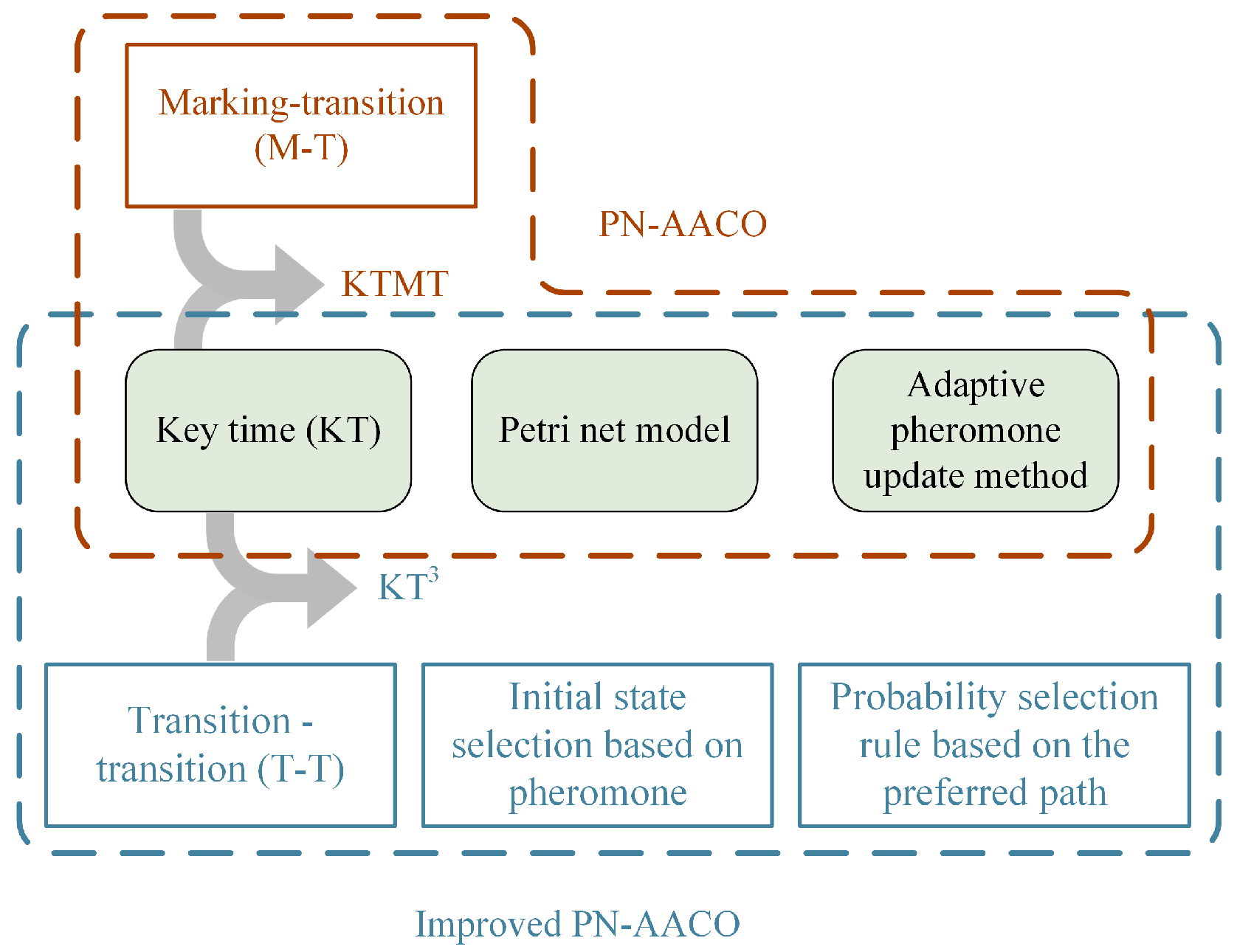
The improved algorithm primarily improves the initial state selection method, recording method, and update method of the pheromones, as shown in Figure 1 when compared with the original algorithm.

As has been explained in Section 1.2, Petri nets have their advantages for describing discrete event dynamic systems such as task scheduling and are widely used; the key time point approach can describe the Petri operation process on a global timeline. Therefore, in Figure 1, the iPN-AACO algorithm follows the Petri net model of the original algorithm and the time description of the key time point. The iPN-AACO algorithm changes the original marking–transition (M-T) pheromone index mechanism to transition–transition (T-T) with the size of ${\left|T\right|}^2$ and recollectively with the key time point method as KT³. The benefit of the T-T-based recording method is that it is not affected by the number of Petri net reachable markings, and it does not affect the size of the pheromone recording as the number of states increases. However, this also brings a disadvantage because the indexing of the pheromone markings has an uncertainty, i.e., the markers may be different between the same two transitions. To solve this problem, a probabilistic selection rule based on the best konwn paths was proposed. It makes the algorithm converge according to a heuristic rule. Since the T-T recording method cannot affect the initial selection probability as much as the initial state, a pheromone-based initial state selection method was also proposed. The details are developed and described in the following sections.

3.1. KT³ Method

The key time points serve as a bridge between the Petri net and the algorithm, enabling the optimization of scheduling through these points. The algorithm updates the pheromone levels in each iteration, and how to record pheromones is a crucial optimization issue. In this study, process transitions are analogized to cities in the traveling salesman problem, where each transition serves as a node to record pheromones, resulting in a fixed count of ${\left|T\right|}^2$ pheromones. This pheromone recording table is referred to as the table Eta.

The final sequence formed by the Petri net is actually a finite occurrence sequence $\sigma =M_0{t}_1{M}_1{t}_2{M}_2\dots t_n{M}_n$. The objective is to find a transition sequence ${\sigma }_t=t_1{t}_2\dots t_n$. It is evident that ${\sigma }_t$ is a simplification of $\sigma$, which is obtained by removing states from $\sigma$. If we directly seek ${\sigma }_t$, the marking between any two transitions ordered pair in ${\sigma }_t$ in different initial markings is indeterminate. Therefore, using the transition–transition pheromone index mechanism does not uniquely describe the states in principle, but only reflects the “distance” between transitions locally. This leads to the ant’s selection based on the pheromones recorded by transition–transition being local. In Section 3.3, we will discuss incorporating the influence of the entire path into the ant’s probability selection.

3.2. Initial State Selection Based on Pheromone

Unlike the random selection of the initial route, the convergence ability of the algorithm will be reduced if the route is influenced by the best known route and the initial selection is still random. So, the first transition from each job $J_i$ is extracted to form the initial variation set $T_o$. Simultaneously, maintain a table Zeta of size $\left|T_o\right|$ to record the initial pheromone levels. At the beginning of each ant’s traversal, the k-th ant (where $k=1,2,\dots ,m$) selects the initial city according to a random proportion rule. The probability of selecting a particular transition is designed as follows:

$$p_i\left(t\right)=\left\{\begin{array}{c}{\displaystyle \frac{{\left[{\varsigma }_i\left(t\right)\right]}^{\alpha }{{\lambda }_i}^{\beta }}{{\displaystyle \sum _{s\in T_o}}{\left[{\varsigma }_s\left(t\right)\right]}^{\alpha }{{\lambda }_s}^{\beta }}},i=1,2,\dots ,\left|T_o\right|\hfill \\ 0,\mathrm{other}\hfill \end{array}\right.$$

(6)

where ${\varsigma }_i\left(t\right)$ represents the pheromone level on transition $t_i$ selected in the initial marking $M_0$.

3.3. Probabilistic Selection Rules Based on Best Known Paths

In Equation (2), the factor ${\left[{\lambda }_{i,j}\left(t\right)\right]}^{\beta }$ is only the time-consuming impact of local transition. Obviously, it is inappropriate to have only the local transition time affecting the selection probability in the whole path, and the path selection of ants should take into account the path impact of the shortest time-consuming path in each round. After each iteration $n_c(n_c=1,2,\dots ,N_c)$ is completed, the shortest path ${\sigma }_{tBest}$ with the least execution time is retained. When $n_c\ge 2$, the probability selection of each ant is influenced by the global best known path. The rule for designing probability selection is as follows:

$$p_{i,j}\left(t\right)=\left\{\begin{array}{c}[1+\Lambda ]·{\displaystyle \frac{{\left[{\eta }_{i,j}\left(t\right)\right]}^{\alpha }{{\lambda }_j}^{\beta }}{{\displaystyle \sum _{s\in a_k}}{\left[{\eta }_{i,s}\left(t\right)\right]}^{\alpha }{{\lambda }_s}^{\beta }}},j\in a_k\hfill \\ 0,\mathrm{other}\hfill \end{array}\right.$$

(7)

where $\Lambda$ is the global best known path influence component, which is designed to influence as follows:

$$\Lambda =sgn(n_c-1)·Q·{\displaystyle \frac{n_c^3}{N_c/2}}·{(\epsilon +\xi )}^z$$

(8)

where $N_c$ is the maximum count of iterations; $\epsilon$ represents the overlap between the current path and the best known path; and Algorithm 1 shows how to compute $\epsilon$.

Algorithm 1 Compute $\epsilon$.

Require: transition sequence of current path ${\sigma }_t^{cur}$, transition sequence set of global best known path ${\sigma }_t^{best}=\{{\sigma }_{t1}^{best},{\sigma }_{t2}^{best},\cdots ,{\sigma }_{tmax}^{best}\}$.

Ensure: $\epsilon$;

1: for $i=1$; $i⩽\left|{\sigma }_t^{best}\right|$; $i++$do

2:       if ${\sigma }_t^{cur}$ begin with ${\sigma }_{ti}^{best}$ then

3:            Compute $\epsilon ={\displaystyle \frac{\left|{\sigma }_t^{cur}\right|}{\left|{\sigma }_t^{best}\right|}}$;▹$\left|{\sigma }_t\right|$ denotes the number of transitions in the sequence

4:            break;

5:      end if

6: end for

7: return $\epsilon$;

$\xi$ is the overlap compensation coefficient, and z is the overlap influence coefficient. The factor $sgn(n_c-1)$ is to present the effect of the best known path at the first iteration, where only the first round of paths are traveled, and the path with the shortest time to execute the sequence occurs. The factor $n_c^3/(N_c/2)$ is applied to allow the ant colony to accelerate the rate of convergence as the count of iterations increases. The influence of the real best known path on the ant selection probability is the factor ${(\epsilon +\xi )}^z$. After many tests, it was summarized that it would be more appropriate to take $\xi =0.5$ and $z=1.5$ in this study.

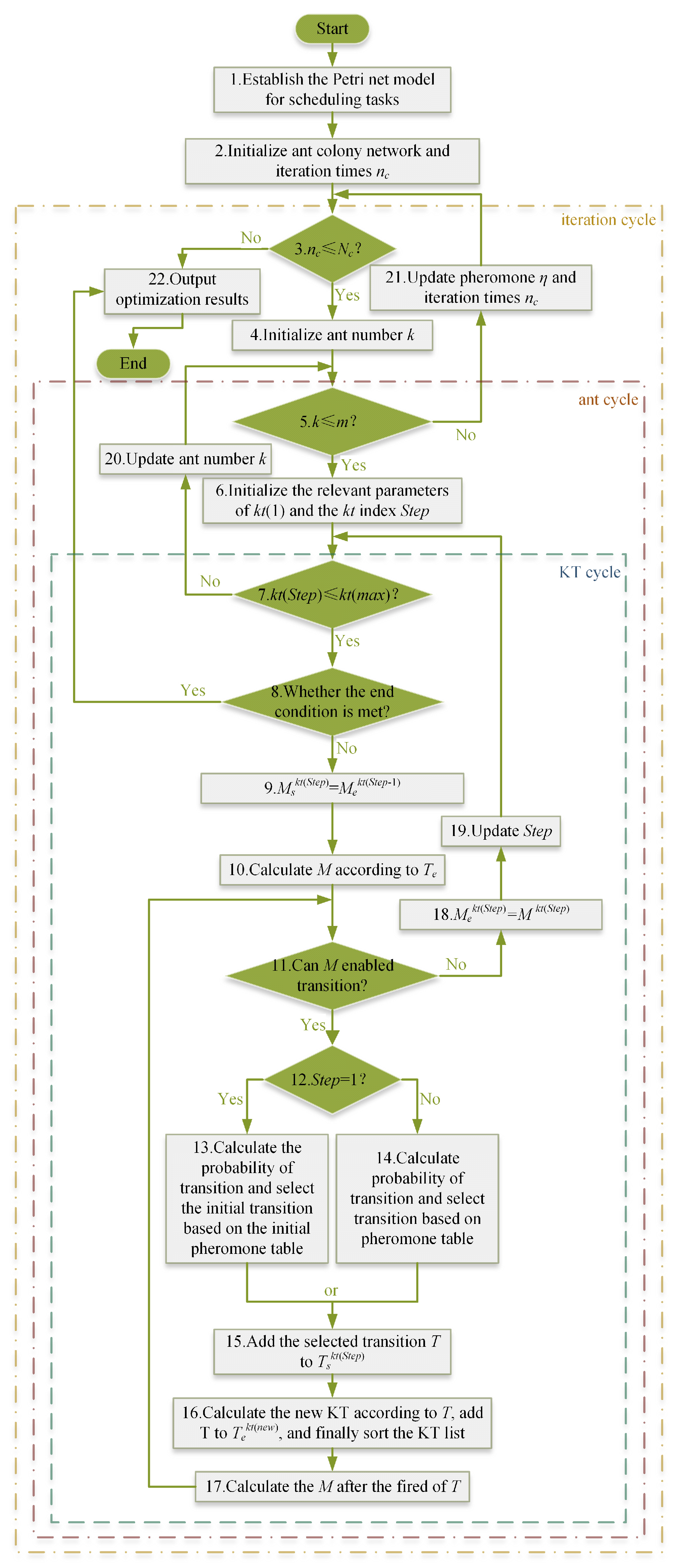
4. Improved Algorithmic Flow

The original PN-AACO algorithm process maintained two tables: the table KT and the pheromone table Eta. The iPN-AACO algorithm also includes an additional table: the initial pheromone table Zeta. The improved algorithm achieves optimization through an iteration cycle, ant cycle, and KT cycle, as illustrated in the Figure 2.

From Figure 2, it can be observed that the algorithm process mainly consists of three stages: model building, initialization, and cycle body.

Modeling of the Petri net for scheduling tasks in done in step 1. Find $M_n$ using a method where each job is completed individually and sequentially to ensure that $M_n$ is reachable. The scheduling process is described in the Petri net model to determine data such as P, T, $C^{+}$, $C^{-}$, $T_{\tau }$, $T_o$, $M_0$, etc., to prepare the data input for the next ACO algorithm.

Step 2 is ACO algorithm initialization. In this step, some parameters are defined, including m, $\lambda$, $\alpha$, $\beta$, $\rho$, Q, and $\gamma$. Then, create the table KT, table Eta, table Zeta, and tables for some intermediate parameters. Finally, set the iteration times to 1 and prepare the first iteration.

The three-layer cycle is described as follows: The three cycles are, in order from outside to inside, the iteration cycle, the ant cycle and the KT cycle. First, outside the cycle, initialize the iterations $n_c$. After entering the iteration cycle, i.e., step 3, first determine whether the current iteration count is less than or equal to the specified count of cycles; if not, enter step 22—output the result and end the cycle. If yes, enter step 4—initialize the ant number $k=1$, and enter the ant cycle, i.e., step 5. In the ant cycle, the count of ants is m. If all ants are traveled, enter step 21—the pheromone level is updated according to Equations (3) and (5) and $n_c$ increases itself by one to the next iteration cycle; if not traveled completely, enter step 6—initialize $Tim{e}^{kt\left(1\right)}=0$, $M_s^{kt\left(1\right)}=M_e^{kt\left(0\right)}=M_0$, $T_e^{kt\left(1\right)}=\Phi$, and prepare to enter the KT cycle, where $Step$ is the index of KT; initialize index $Step=1$.

Enter the KT cycle, i.e., step 7, to determine whether the current is the last key time point of the table KT. If yes, then enter step 20—jump out of the KT cycle to update the ant index number to travel the new ant; if not, then enter the KT cycle body, i.e., step 8. Because each ant does not necessarily travel through the same number of key time points, the ant cycle is in the outer layer of the KT cycle. The KT cycle needs to traverse all key time points on the global timeline, and the key time points are dynamically increasing. After entering the KT cycle, it first determines whether the end condition is satisfied in step 8, and the end condition can determine whether the end marking $M_n$ is reached. Output the optimization result in step 22 if the end state is satisfied; if not, continue the KT cycle, i.e., step 9. When traveling to $kt\left(Step\right)$, the following is satisfied:

$$M_s^{kt\left(Step\right)}=M_e^{kt(Step-1)},Step=1,2,\dots ,max$$

(9)

Then, enter step 10 according to the following:

$$M^{kt\left(Step\right)}=M_s^{kt\left(Step\right)}+C^{+}{U}_{T_e}$$

(10)

Compute the $M^{kt\left(Step\right)}$ values, where $U_{T_e}$ is a vector of which the ordinal labeling set is the transition set $T_e^{kt\left(Step\right)}$. The element of $U_{T_e}$ is the fired count of the transition corresponding to the same ordinal labeling. For example, if the count of a transition set is $\left|P\right|=3$, then $T_e^{kt\left(Step\right)}=\{t_1,t_1,t_2,t_2,t_2,t_3\}$. Then, $U_{T_e}={[2,3,1]}^T$. After calculating $M^{kt\left(Step\right)}$, enter step 11: Determine what transition can fire in $M^{kt\left(Step\right)}$. The basis on which the transition $t_j$ can fire is

$$\bigcap _{i=1}^{\left|P\right|}{M}_i^{kt\left(Step\right)}\ge C_{ij}^{-}$$

(11)

where $M^{kt\left(Step\right)}$ is a vector, $M_i^{kt\left(Step\right)}$ denotes the i-th element of $M^{kt\left(Step\right)}$, and similarly, $C_{ij}^{-}$ denotes the i-th row and j-th column of matrix $C^{-}$. If Equation (11) is satisfied, then the transition can fire. Temporary transitions that can occur are stored, and the process proceeds to step 12. If $Step=1$, then proceed to step 13, where the probabilities are computed based on Equation (6), and an initial transition is randomly selected. Otherwise, proceed to step 14, where computations and selections are made according to Equation (7). Assuming that the chosen transition is $t_j$, then a new element $t_j$ is added to $T_s^{kt\left(Step\right)}$ in step 15, i.e.,

$${T^{\prime }}_s^{kt\left(Step\right)}=T_s^{kt\left(Step\right)}\cup t_j$$

(12)

where “′” represents the new value. Once it is added, go to step 16. If $Tim{e}^{kt\left(Step\right)}+{\tau }_j$ does not exist in the table KT, add $Tim{e}^{kt\left(Step\right)}+{\tau }_j$ to the table KT and sort by $Time$. Also, update the member variable $T_e$ of the table KT for the new moment:

$${T^{\prime }}_e^{KT(Tim{e}^{kt\left(Step\right)}+{\tau }_j)}=T_e^{KT(Tim{e}^{kt\left(Step\right)}+{\tau }_j)}\cup t_j$$

(13)

Next, enter step 17: Calculate the new $M^{kt\left(Step\right)}$ after the transition has fired. It is defined as follows:

$${M^{\prime }}^{kt\left(Step\right)}=M^{kt\left(Step\right)}-C^{-}{U}_{t_j}$$

(14)

where $U_{t_j}$ is a vector with the transition $t_j$ as the ordinal labeling set. After calculating the new $M^{kt\left(Step\right)}$, we again determine whether $M^{kt\left(Step\right)}$ can fire the transition or not. Until $M^{kt\left(Step\right)}$ is unable to fire, enter step 18. Throughout the process from step 11 to step 17, the tokens always satisfy the selected transition first, and after the current transition has consumed the tokens, the remaining tokens are judged to determine whether a new transition can still fire. This process can effectively prevent the deadlock phenomenon caused by resource grabbing. Next is step 19: $M_e^{kt\left(Step\right)}=M^{kt\left(Step\right)}$ is updated, while $Step$ increments itself by one and goes to the next KT cycle.

5. Performance Proof

The experimental setup utilized an 3.0 GHz processor with 32 GB RAM. MATLAB r2022a was employed as the simulation software. To validate the effectiveness of the iPN-AACO algorithm, two simulations were conducted and compared with the original method (in references) and PN-AACO algorithm. The objective of the algorithms was to find a scheduling solution that minimizes the completion time ${\tau }_{sum}$ of the system’s tasks, i.e., to find the shortest transition sequence ${\sigma }_t$ that minimizes the ${\tau }_{sum}$.

5.1. Radar Receiver Test Task

This simulation used the Petri net in reference [17], which is a parallel test of five parameters of radar receivers A and B (corresponding to tasks $J_1$ and $J_2$) with five types of instrumentation needed to complete the test. The S³PR model established in reference [17] has a high number of states due to different model types, but the essence is to split a transition into a combination of immediate and timed transitions. The network established in this study needs to combine the corresponding immediate and timed transitions, and the final TPN model is shown in Figure 3. In the model, $P=\{p_1,p_2,\dots ,p_{12}\}$, $T=\{t_1,t_2,\dots ,t_{10}\}$, and $R=\{r_1,r_2,r_3,r_4,r_5\}=\{p_{13},p_{14},p_{15},p_{16},p_{17}\}\in P$. The transition time $\tau$ is calculated as

$$\tau =\{7,4,8,3,5,8,3,3,7,6\}$$

(15)

Set the initial and end markings as

$$\begin{array}{c}{M}_0=\{1,0,0,0,0,0,1,0,0,0,0,0,1,1,2,1,1\}\hfill \\ M_n=\{0,0,0,0,0,1,0,0,0,0,0,1,1,1,2,1,1\}\hfill \end{array}$$

(16)

The equivalent initial and end markings in reference [17] are, respectively,

$$\begin{array}{c}{M}_0^{ref}=\{1,0,0,0,0,0,0,0,0,0,1,0,0,0,0,0,0,0,0,0,1,1,2,1,1\}\hfill \\ M_n^{ref}=\{0,0,0,0,0,0,0,0,0,1,0,0,0,0,0,0,0,0,0,1,1,1,2,1,1\}\hfill \end{array}$$

(17)

The algorithm parameters were set as follows: the maximum iteration count $N_c=50$, $m=30$, $\alpha =1.9$, $\beta =0.4$, $\rho =0.15$, $Q=1000$, and $\gamma =0.45$. In the iPN-AACO algorithm, $T_o=\{t_1,t_6\}$. It was run 20 times, and the results obtained are shown in

Table 1. Comparison results in test task.

Method	Best Known Sequence	Sequence Probability	Execution Time/s	Iterations
PSO				28
GA-ACO	$t_{10}{t}_{20}{t}_{15}{t}_{25}{t}_{11}{t}_{21}{t}_{16}{t}_{26}{t}_{12}{t}_{22}-$$t_{17}{t}_{27}{t}_{18}{t}_{28}{t}_{13}{t}_{23}{t}_{19}{t}_{29}{t}_{14}{t}_{24}$	95%	37	25
GA-PSO				22
PN-AACO	$t_1{t}_6{t}_2{t}_7{t}_3{t}_8{t}_9{t}_4{t}_{10}{t}_5$	100%	37	1
iPN-AACO	$t_1{t}_6{t}_2{t}_7{t}_3{t}_8{t}_9{t}_4{t}_{10}{t}_5$	100%	37	1

.

The five methods of PSO, GA-ACO, GA-PSO, PN-AACO, and iPN-AACO to obtain the best known ${\sigma }_t$ were practically the same; as an example of iPN-AACO, the resulting Gantt chart of the task scheduling sequence is shown in Figure 4.

The comparison shows that all five methods could find the optimal sequence with a ${\tau }_{sum}$ of 37 s. However, the proposed two algorithms could find the best known path in the first iteration, which was 95% shorter than the 22 times in the GA-PSO algorithm proposed in reference [17]. Because the algorithm in this study uses the key time points method, many unreasonable paths are avoided at the beginning of using the ACO algorithm, making the final path only one.

To verify the advantage of the iPN-AACO algorithm in terms of computational speed in the face of an increase in the token number, the five initial markings $M_0$ used for the experiment were the following:

$$\begin{array}{cc}\hfill M_0=& [1,0,0,0,0,0,1,0,0,0,0,0,1,1,2,1,1],\hfill \\ \hfill & [2,0,0,0,0,0,1,0,0,0,0,0,1,1,2,1,1],\hfill \\ \hfill & [2,0,0,0,0,0,2,0,0,0,0,0,1,1,2,1,1],\hfill \\ \hfill & [3,0,0,0,0,0,3,0,0,0,0,0,1,1,2,1,1],\hfill \\ \hfill & [5,0,0,0,0,0,5,0,0,0,0,0,1,1,2,1,1].\hfill \end{array}$$

(18)

Each $M_0$ was run 10 times, and the final results are shown in

Table 2. Comparison of test task.

Method	PN-ACOO					iPN-ACOO
Initial token count 1	2	3	4	6	10	2	3	4	6	10
${\tau }_{best}$ 2/s	37	47	59	87	43	37	47	59	87	43
Hit rate	100%	100%	100%	100%	100%	100%	100%	100%	100%	100%
${\tau }_{best}$ convergence rate	100%	100%	100%	100%	100%	100%	100%	100%	100%	100%
${\tau }_{best}$ iterations	1	1	1	1	1	1	1	1	1	1
${\tau }_{ave}$ 3 convergence rate	100%	100%	100%	100%	100%	100%	100%	100%	100%	100%
${\tau }_{ave}$ iterations	1	4.6	4.7	5.5	5.2	1	3.2	9.33	15.9	23.6
Pheromone size	14	72.3	130.2	514	2053.7	102	102	102	102	102
Execution time/s	0.38	1.26	2.21	6.71	34.15	1.16	1.72	2.39	3.67	7.12

¹ Non-resources. ² Best known completion time. ³ Average completion time.

. Unless otherwise specified, all parameters refer to the average values obtained from 10 runs. The search hit rate indicates that the proportion of times of the minimum completion time was found in 10 runs. The best known and average completion time iteration counts refer to the average number of iterations for convergence.

According to Table 2, both algorithms converged to the same ${\tau }_{best}$, and both were able to find ${\tau }_{best}$ completely. Due to the relatively simple system structure, both algorithms could find ${\tau }_{best}$ in the first iteration and converge. The ${\tau }_{best}$ and ${\tau }_{ave}$ convergence rates were both 100%; however, with an increase in the initial token count, the iPN-AACO algorithm required more ${\tau }_{ave}$ iterations to converge. Nevertheless, ${\tau }_{ave}$ does not have practical significance. When it does not converge, it only indicates that the algorithm is still searching. With the initial token count of 2, the execution time of the iPN-AACO algorithm increased by 205% compared to PN-AACO. But when the initial token count was 10, the program execution time of iPN-AACO decreased by 79% compared to PN-AACO. This indicates that as the initial token count increases, the pheromone size in the PN-AACO algorithm increases significantly, which has a significant impact on the PN-AACO algorithm based on the count of states. However, the iPN-AACO algorithm, with a fixed count of pheromones, achieved higher efficiency in execution. A comparison of program execution times is shown in Figure 5.

According to Figure 5, the PN-AACO algorithm exhibited faster program execution times than the iPN-AACO algorithm when the initial token count was 2, 3, and 4. As the initial token count increased, the program execution time of the PN-AACO algorithm grew exponentially due to the growth in Petri net states. In contrast, the iPN-AACO algorithm maintained a relatively stable execution time because the pheromone size remained constant. This advantage positions the iPN-AACO algorithm favorably in scenarios involving large-scale systems with multiple states. Both algorithms generally operated around the boundary of the pheromone size given by ${\left|T\right|}^2+\left|T_o\right|$. Differences in performance may arise due to variations in coding methods such as concatenation functions and array manipulations.

5.2. Manufacturing System Processing Task

This simulation utilized the model depicted in Figure 6 of reference [25]. The model represents a manufacturing system with four machining tasks and is constrained by three shared resources. In this model, the sets are defined as follows: $P=\{p_1,p_2,\dots ,p_{20}\}$, $T=\{t_1,t_2,\dots ,t_{18}\}$, and $R=\{r_1,r_2,r_3\}=\{p_{18},p_{19},p_{20}\}\in P$. The transition time ${\displaystyle \frac{1}{\lambda }}$ is represented by

$${\displaystyle \frac{1}{\lambda }}=\{69,75,85,57,51,80,75,97,85,92,98,78,75,56,70,68,99,76,93\}$$

(19)

The initial and end markings in reference [25] are, respectively,

$$\begin{array}{c}{M}_0=\{1,1,1,1,0,0,0,0,0,0,0,0,0,0,0,0,0,0,1,1,1\}\hfill \\ M_n=\{0,0,0,0,0,0,0,0,0,0,0,0,0,0,1,1,1,1,1,1,1\}\hfill \end{array}$$

(20)

The algorithm simulation parameters were the same as the radar receiver test task. In the iPN-AACO algorithm, $T_o=\{t_0,t_1,t_6,t_{11},t_{16}\}$. The two algorithms, PN-AACO and iPN-AACO, were run 20 times each and compared with the data from the reference [25] species, and the results are shown in

Table 3. Results of the three algorithms.

Method	Improved ACO	PN-AACO	iPN-AACO
${\tau }_{ave}$ iterations	5.2	1.4	1
${\tau }_{best}$ iterations	3	1	1
${\tau }_{ave}$/s	427	427.3	427
${\tau }_{best}$/s	427	427	427
Hit rate	100%	100%	100%

.

From Table 3, it can be seen that, compared to the improved ACO algorithm, the PN-AACO algorithm shortened the ${\tau }_{ave}$ iterations and the ${\tau }_{best}$ iterations by 73% and 67%, respectively, and the iPN-AACO algorithm shortened the ${\tau }_{ave}$ iterations and the ${\tau }_{best}$ iterations by 81% and 67%, respectively. The two algorithms proposed converged more quickly. What can be seen is that the PN-AACO algorithm was more volatile. The iPN-AACO performed slightly better in the optimization problem for this model. In the parameter of ${\tau }_{ave}$, convergence to a stable value is not of practical significance; only PN-AACO converged to a minimum value near 427 and performed a local search. All three algorithms were identical in the two metrics of ${\tau }_{best}$ and the hit rate. Finally, the improved ACO algorithm found the best known transition sequence $t_1{t}_{16}{t}_{11}{t}_{17}{t}_{18}{t}_2{t}_5{t}_6{t}_8{t}_{12}{t}_{15}{t}_9$. The PN-AACO algorithm and the iPN-AACO algorithm found more than one best known transition sequence, and the Gantt chart of the best known scheduling is shown in Figure 7, taking one sequence of $t_1{t}_{16}{t}_{11}{t}_{17}{t}_6{t}_{18}{t}_2{t}_8{t}_{12}{t}_5{t}_9{t}_{15}$ as an example.

In order to verify the advantage of the iPN-AACO algorithm in terms of computational speed in the face of increasing token number, the two methods of PN-AACO and the iPN-AACO were used in the initial markings $M_0$ of

$$\begin{array}{cc}\hfill M_0=& [1,1,1,1,0,0,0,0,0,0,0,0,0,0,0,0,0,0,1,1,1],\hfill \\ \hfill & [2,1,1,1,0,0,0,0,0,0,0,0,0,0,0,0,0,0,1,1,1],\hfill \\ \hfill & [2,2,1,1,0,0,0,0,0,0,0,0,0,0,0,0,0,0,1,1,1],\hfill \\ \hfill & [2,2,2,2,0,0,0,0,0,0,0,0,0,0,0,0,0,0,1,1,1],\hfill \\ \hfill & [3,3,3,3,0,0,0,0,0,0,0,0,0,0,0,0,0,0,1,1,1].\hfill \end{array}$$

(21)

In this testing, the algorithm parameters were the same as in radar receiver test task. We executed 10 times for each $M_0$, and the final results are presented in

Table 4. Comparison of processing task.

Method	PN-ACOO					Improved PN-ACOO
Initial token count	4	5	6	8	12	4	5	6	8	12
${\tau }_{best}$/s	427	512	581	762	1175	427	512	581	762	1097
Hit rate	100%	60%	60%	10%	0%	100%	60%	50%	70%	40%
${\tau }_{best}$ convergence rate	100%	100%	80%	80%	N/A	100%	100%	90%	100%	10%
${\tau }_{best}$ iterations	1.2	2.4	2.9	2.75	N/A	1.3	3.6	2.3	10.5	29
${\tau }_{ave}$ convergence rate	60%	10%	10%	0%	N/A	50%	30%	10%	20%	0%
${\tau }_{ave}$ iterations	12.3	8	10	Inf	N/A	10.8	6.3	14	29.5	Inf
Pheromone size	209.9	478.6	896.7	1606.4	3149.9	366	366	366	366	366
Execution time/s	1.45	3.28	6.23	14.00	36.90	1.39	1.63	1.76	2.45	3.10

.

According to Table 4, it is evident that compared to the iPN-AACO, the PN-AACO algorithm failed to find the best known completion time when the initial token count was 12, and the search hit rate decreased as the initial token count increased. Conversely, the iPN-AACO algorithm exhibited fluctuating search hit rates as the initial token count increased. Both algorithms showed decreasing convergence rates for ${\tau }_{best}$ and ${\tau }_{ave}$ as the initial token count increased, with the iPN-AACO algorithm requiring more iterations. The processing task, compared to test task, represents a more complex system, where increasing the initial token count results in more states. Consequently, both algorithms’ search comprehensiveness capacities were affected, leading to a decline in performance with increasing initial token count. However, the data indicate that the iPN-AACO algorithm performed slightly better. The increase in initial token count led to an increase in the pheromone size in PN-AACO, thereby increasing both algorithms’ execution times. With the initial token count of 4, the execution time of the iPN-AACO algorithm decreased by 4% compared to PN-AACO. And when the initial token count was 12, the program execution time of iPN-AACO decreased by 92% compared to PN-AACO. Similar to the test task, this suggests that the iPN-AACO’s efficiency increases with an increase in the initial token count.

6. Train Loading Application

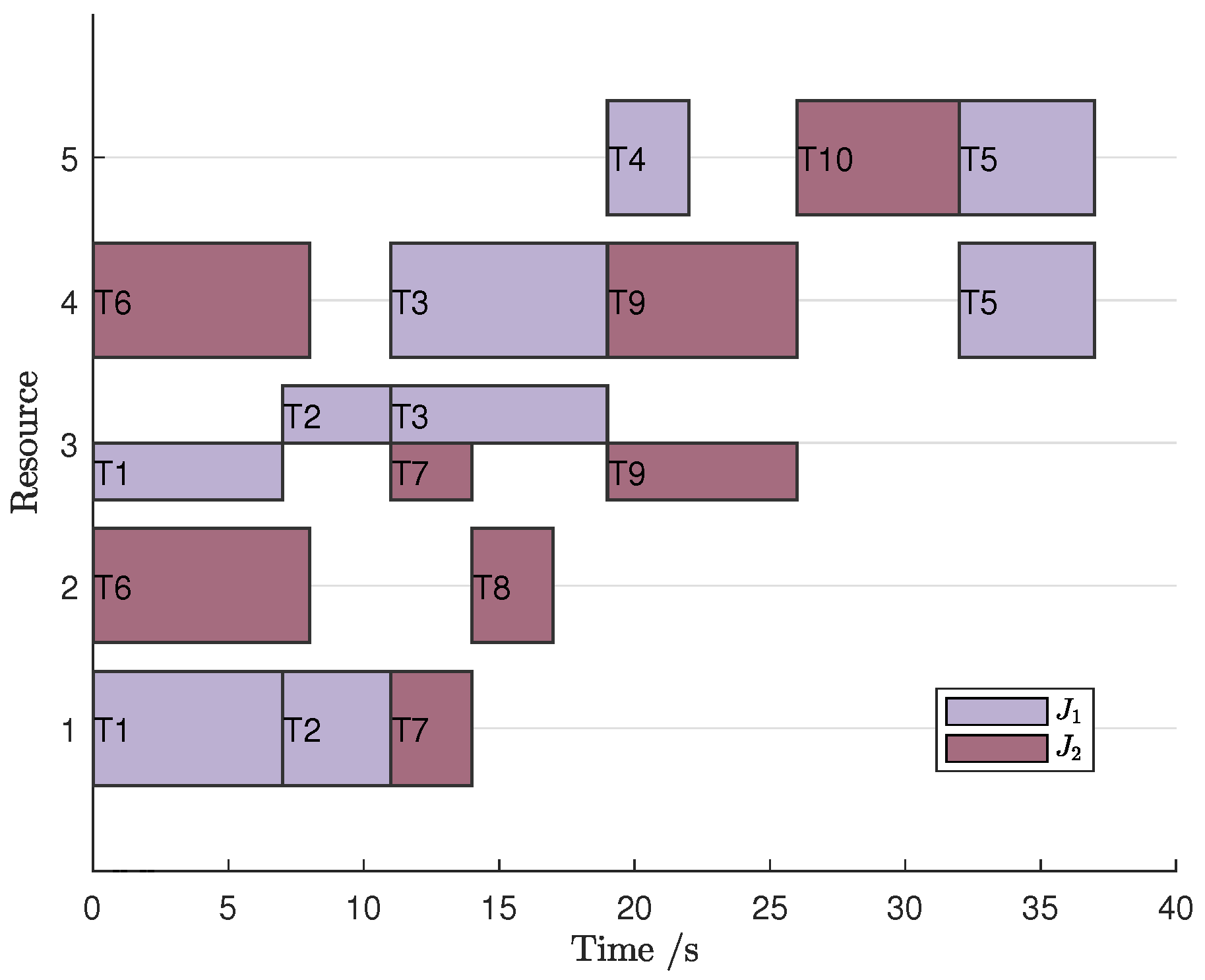
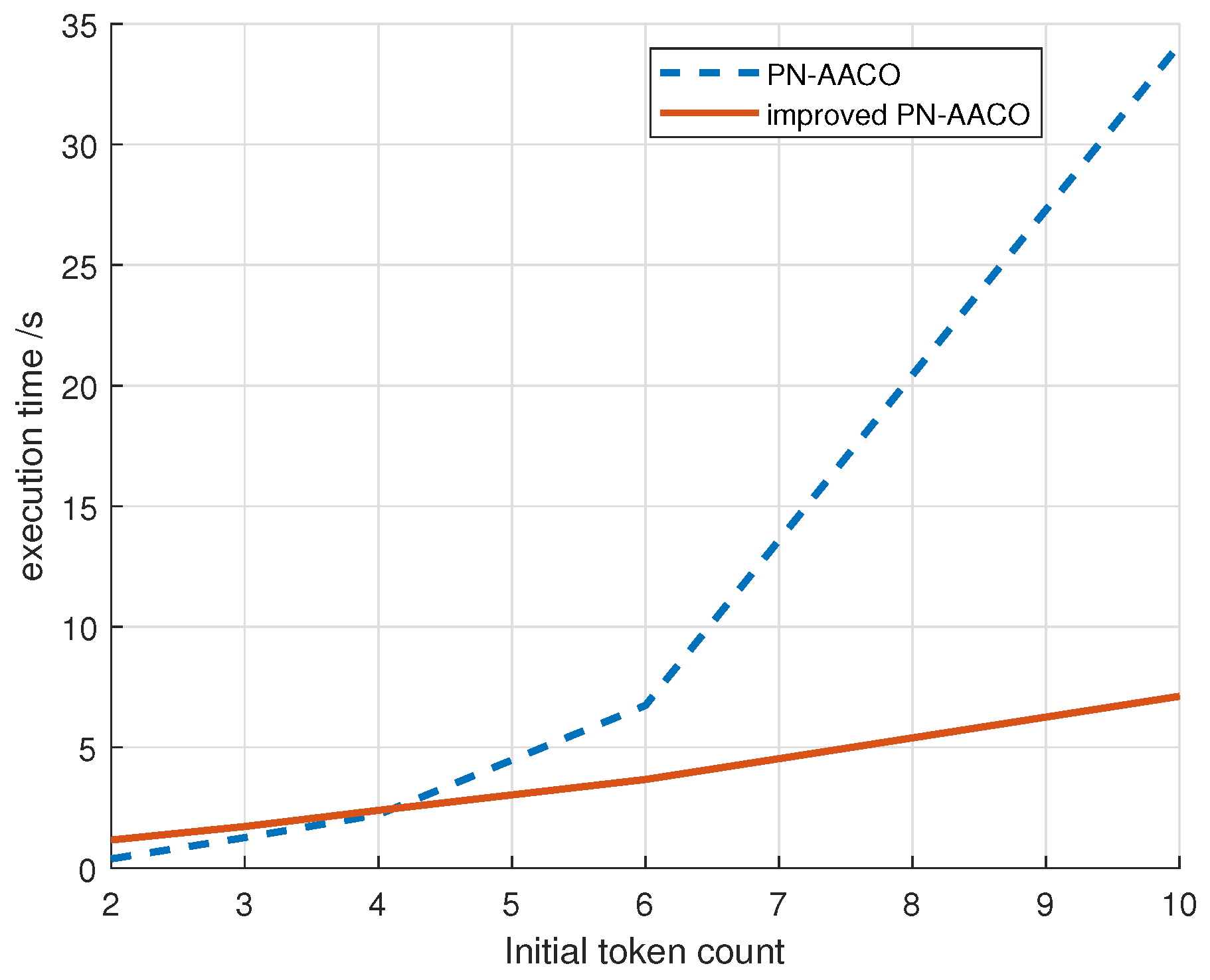
To validate the feasibility of the iPN-AACO algorithm, this study conducted a simulation using the task of coiling carbon steel sheets in the 2# warehouse area of the Finished Product Service Branch of Gansu Jiuquan Iron and Steel Group Hongxing Iron and Steel Co., Ltd., Jiayuguan, China. The simulation aimed to obtain a scheduling solution for minimizing the completion time of work in this system. Specifically, the goal was to find the shortest transition sequence ${\sigma }_t$ that minimized the completion time ${\tau }_{sum}$. The simulation employed both the PN-AACO algorithm and the iPN-AACO algorithm for this purpose.

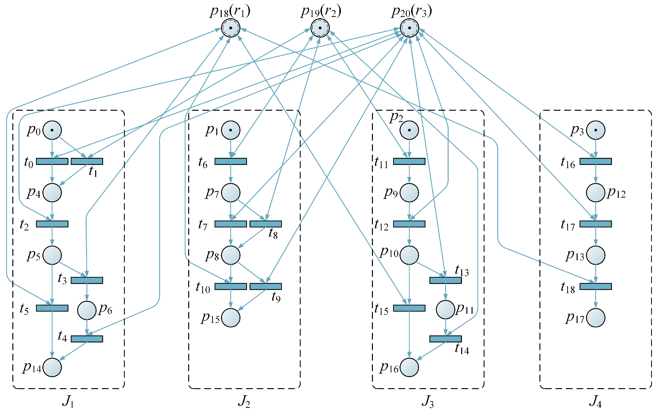
There are two double-girder overhead traveling cranes and two forklifts for transporting steel coils in the cold rolled carbon steel sheet 2# storage area. And there is one railroad loading and unloading line with access to the warehouse area with six carriages, one carriage for two steel brackets and one steel bracket for two steel coils. The task was to optimize the deployment of cranes and forklifts in such a way that the shortest possible time was required for loading the six carriages of steel coils that were driven into the storage area. This study did not take into account the mutual interference between cranes, and it assumed that the storage capacity is much greater than the capacity of the six carriages. Additionally, it did not consider the time taken for the train to transport coils to the next empty train position. The loading problem was simplified to model the Petri net, as shown in Figure 8.

The description of each parameter in Figure 8 is shown in

Table 5. Definition of places and transitions.

Places or Transitions	Descriptions
$p_1,p_4,p_7,p_{10},p_{13},p_{16}$	Count of steel brackets
$p_2,p_5,p_8,p_{11},p_{14},p_{17}$	Count of steel coils
$p_3,p_6,p_9,p_{12},p_{15},p_{18}$	Completion status of coil loading
$p_{10}\left(r_1\right),p_{11}\left(r_2\right)$	Crane resources, forklift resources, respectively
$t_1,t_5,t_9,t_{13},t_{17},t_{21}$	Average time for crane to install steel bracket: 90 s
$t_2,t_6,t_{10},t_{14},t_{18},t_{22}$	Average time for forklift to install steel bracket: 120 s
$t_3,t_7,t_{11},t_{15},t_{19},t_{23}$	Average time for crane loading steel coil: 150 s
$t_4,t_8,t_{12},t_{16},t_{20},t_{24}$	Average time for forklift loading steel coil: 180 s

.

The algorithm parameters were the same as in test task. In the iPN-AACO algorithm, $T_o=\{t_1,t_2,t_5,t_6,t_9,t_{10},t_{13},t_{14},t_{17},t_{18},t_{21},t_{22}\}$. Our target was to find an ${\sigma }_t$ that minimizes the ${\tau }_{sum}$ when the train drives into the warehouse area. The PN-AACO and iPN-AACO algorithms were used, where the PN-AACO algorithm had a execution time of 36.1 s, and the iPN-AACO algorithm had a execution time of 5.1 s. 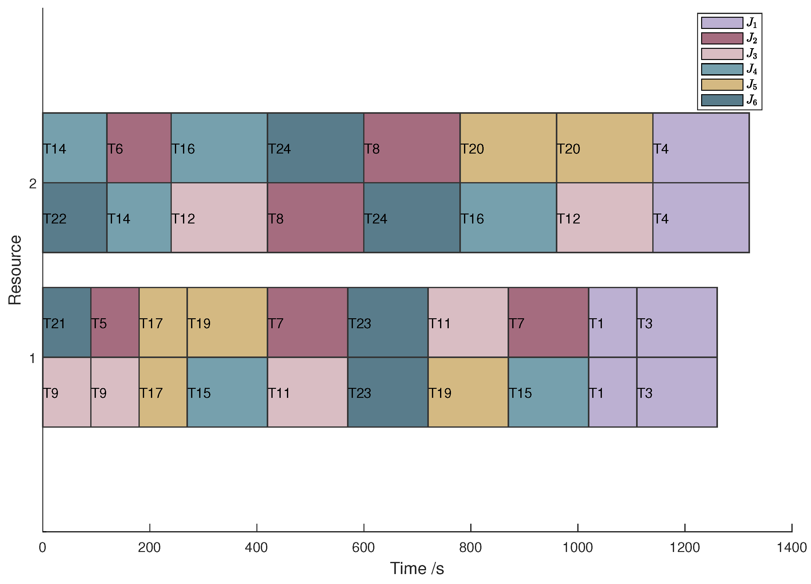Both algorithms searched for the best known path, and the ${\tau }_{sum}$ of ${\sigma }_t$ came out ot 1320 s. It can be seen from the algorithms that there is more than one best known path, and the scheduling Gantt chart is shown in Figure 9 for example $t_{22}{t}_9{t}_{21}{t}_{14}{t}_9{t}_5{t}_{14}{t}_6{t}_{17}{t}_{17}{t}_{12}{t}_{16}{t}_{15}{t}_{19}{t}_8{t}_{11}{t}_7{t}_{24}{t}_{23}{t}_{23}{t}_{24}{t}_8{t}_{19}{t}_{11}{t}_{16}{t}_{20}{t}_{15}{t}_7{t}_{12}{t}_{20}{t}_1{t}_1{t}_3{t}_3{t}_4{t}_4$.

7. Conclusions

This study introduces the iPN-AACO algorithm to address the performance issues encountered by the original PN-AACO algorithm when the model size or state increases. The iPN-AACO algorithm retains the Petri net modeling method and the time representation of key time points. On this basis, the pheromone index mechanism and the initial state selection method were improved so that the pheromone size was fixed to ${\left|T\right|}^2+\left|T_o\right|$. After that, a probabilistic selection method based on best known paths was designed to increase the influence of the best known paths and weaken the local influence on the results. Finally, through simulations, it has been demonstrated that the PN-AACO algorithm exhibited faster program execution speeds in scenarios with small-scale models or fewer states. In contrast, the iPN-AACO algorithm was faster when the model size or state increased, with up to a 92% reduction in runtime in the simulations. Each algorithm presents its own advantages when confronted with different application environments, necessitating the selection based on the specific task requirements. The next task will be to deploy the algorithms in the edge control nodes (self-developed PAG series controllers), and how to UI the modeling work is also a key point to consider.