AFEDet: A Symmetry-Aware Deep Learning Model for Multi-Scale Object Detection in Aerial Images

Abstract

Traditional convolutional neural networks face challenges in handling multi-scale targets in remote sensing object detection due to fixed receptive fields and simple feature fusion strategies, which affect detection accuracy. This study proposes an adaptive feature extraction object detection network (AFEDet). Compared with previous models, the design philosophy of this network demonstrates greater flexibility and complementarity. First, parallel dilated convolutions effectively expand the receptive field to capture multi-scale features. Subsequently, the channel attention gating mechanism further refines these features and assigns weights based on the importance of each channel, enhancing feature quality and representation ability. Second, the multi-scale enhanced feature pyramid network (MeFPN) constructs a structurally symmetrical bidirectional transmission path. It aligns multi-scale features in the same semantic space using linear transformation, reducing scale bias and improving representation consistency. Finally, the scale adaptive loss (SAL) function dynamically adjusts loss weights according to the scale of the target, guiding the network to learn features of different scale targets evenly during training and optimizing the model’s learning direction. The proposed architecture inherently integrates symmetry principles through its bidirectional feature fusion paradigm and equilibrium-seeking mechanism. Specifically, the symmetric structure of MeFPN balances information flow between shallow and deep features, while SAL applies a symmetry-inspired loss-weighting strategy to maintain optimization consistency across different scales. Experimental results show that, on the DOTA dataset, the proposed method improves the mAP by 7.12% compared to the baseline model.

1. Introduction

The main task of remote sensing target detection is to accurately identify the categories and locations of objects in remote sensing images [1]. It has a wide range of application fields, including but not limited to military and mineral exploration [2]. Due to the growth of deep learning, convolutional neural networks (CNNs) can play a vital role in remote sensing image analysis because of their powerful feature-learning capabilities. CNN can automatically extract hierarchical features of images, thus enabling the recognition and localization of objects in complex backgrounds.

However, conventional object detection approaches encounter numerous challenges when dealing with remote sensing images [3]. As shown in Figure 1, the background of these images is extremely complex, with various terrain elements intertwined, which increases the difficulty of object recognition. Moreover, the scale of objects varies significantly, making it difficult for traditional methods to handle multi-scale objects uniformly and efficiently. Additionally, objects of the same category exhibit significant differences in appearance due to factors such as shooting angles, lighting, and the environment, which pose difficulties for accurate classification.

Research on multi-scale feature representation focuses on two main approaches [4]. One category involves the use of convolution kernels with variable receptive fields, such as dilated convolutions [5] and adaptive pooling techniques [6]. These methods have made some progress in capturing multi-scale features. However, when faced with complex and variable object scales, they still cannot fully cover the required scales, resulting in incomplete feature extraction and thus affecting the detection accuracy. The other category of methods combines hierarchical backbone networks with feature pyramid networks (FPN), which attempt to achieve multi-scale representation by integrating features at different levels [7,8]. In practical applications, due to the structural differences between the two, information loss or misalignment is likely to occur during the feature fusion process [9]. Moreover, the multi-scale feature extraction ability of the backbone network is limited, making it difficult [1] to deal with objects with extreme scale variations. Increasing the number of FPN layers can attempt to solve some problems, but it will increase the model complexity and lead to a large consumption of computing resources.

Figure 1. (a) FPN combined high-level and low-level info via top-down paths and lateral links. (b) PANet [10] added bottom-up paths for bidirectional info flow. (c) BiFPN [11] used weighted feature fusion to enhance the network structure.

Figure 1. (a) FPN combined high-level and low-level info via top-down paths and lateral links. (b) PANet [10] added bottom-up paths for bidirectional info flow. (c) BiFPN [11] used weighted feature fusion to enhance the network structure.

To address the limitations of existing object detection techniques in handling complex scenes and multi-scale targets, this paper proposes an adaptive feature-enhanced detection network (AFEDet). AFEDet addresses the limitations of traditional methods by incorporating dynamic scale selection and bidirectional feature fusion. As shown in Figure 2, the network consists of three main components: adaptive feature extraction (AFE), multi-scale enhanced feature pyramid network (MeFPN), and scale-aware loss (SAL). AFE extracts key features, MeFPN enhances multi-scale fusion, and SAL dynamically adjusts loss weights to optimize training. Experiments show that AFEDet offers key contributions, including:

(1) Flexible Feature Extraction Method: AFE adheres to the principle of operational symmetry. It first employs a sequence of parallel dilated convolutions, expanding the receptive field with minimal computational cost. Then, in the $L_2$-normalization gating module, it introduces a symmetric tanh function, which dynamically adjusts channel weights based on the input features. This mechanism effectively suppresses interference while maintaining a balance between different receptive field branches.

(2) Efficient Feature Fusion Strategy: MeFPN follows the principle of structural symmetry, utilizing linear scale transformation to precisely align upper- and lower-layer feature maps to the middle layer scale. This ensures spatial and semantic consistency across different scales. Unlike traditional FPN, which uses unidirectional information flow, MeFPN employs a symmetric bidirectional transmission path. This design improves fusion efficiency and reduces computational complexity.

(3) Dynamically Adjusted Loss Weights: SAL is designed based on the principle of optimization symmetry, incorporating scale-aware weighting to dynamically adjust loss weights according to target size. During training, it increases the classification and regression loss weight for small objects, enhancing feature learning and detection accuracy.

2. Related Work

2.1. Aerial Object Detection

Traditional deep learning detectors typically use horizontal bounding boxes for object localization. However, in remote sensing imagery, object rotation, dense distribution, and significant aspect ratio variations make it difficult for convolutional networks to extract rotation-invariant features and achieve precise localization [12]. Current research mainly focuses on optimizing rotated bounding boxes and regions and extracting rotation-sensitive features.

Rotated bounding box encoding forms the foundation of rotation-based detection. Early conventional object detection methods, which used horizontal and vertical rectangular boxes, failed to effectively localize rotated objects. The OpenCV representation [13] and long-side representation [14] improved localization accuracy by integrating rotation angles and aspect ratios, laying the groundwork for subsequent research. On this basis, rotated anchor box design has evolved significantly. RRPN [15] was the first to introduce rotated candidate boxes into the RPN [16] architecture, but it suffered from angle discretization limitations. To address this, CSL [17] and DCL [18] reformulated the angle prediction problem as a classification task, while VGL (variance Gaussian labeling) created discrete Gaussian angle labels, successfully overcoming the continuity and periodicity issues associated with regression-based angle prediction. Further improvements include $R^{2}PN$ [14], which introduced multi-directional anchors for specific targets, and $R^{3}Det$ [19], which optimized anchor box design through a feature refinement module and rotation-equivariant networks, significantly improving recall and accuracy. RoI Transformer [20] employed spatial transformation and the RPS-RoI-Align module, enhancing both detection speed and the performance of object classification and boundary regression. AO-RCNN and $R^{2}CNN$ [21] introduced unique network structures and strategies, achieving progress in complex scene detection and small object detection.

2.2. Multi-Scale Object Detection

Multi-scale object detection is a significant challenge in remote sensing image analysis [22]. Traditional FPNs [23] improve detection performance by fusing features from different hierarchical levels [24], yet they still exhibit limitations in complex scenes.

To enhance small-object detection, $R^{2}CNN$ [21] proposed a scale-invariant anchor strategy to accurately locate small objects while utilizing position-sensitive RoI pooling for precise feature extraction. Additionally, DFPN [25] and EFPN [26] introduced improvements in feature extraction enhancement and feature fusion path optimization, respectively. However, these methods fail to achieve high accuracy in large-object detection. The primary reason for this limitation is that the top-down upsampling operation in the FPN can lead to information loss, which in turn causes feature misalignment issues. Info-FPN [27] attempted to enhance feature fusion accuracy by incorporating template matching and feature offset learning, but it still requires further optimization in complex scenes.

To improve large-object detection, attention mechanisms have been introduced. $A^{2}FPN$ [9] utilizes attention mechanisms to focus on key features of large targets, while MSRO-Net [28] adopts a perceptual pyramid feature aggregation module to balance local and global feature extraction, thereby enhancing the representation capability for objects of varying scales. However, these approaches increase computational complexity and require more training data. Despite these improvements, they still do not fully address the limitations of FPN in handling scale diversity.

In contrast, the proposed MeFPN adopts an improved feature fusion strategy. By integrating BFM and leveraging linear scale transformation, MeFPN accurately aligns features across different levels while maintaining a lightweight model design, significantly improving detection accuracy.

2.3. Attention Mechanisms

The attention mechanism mimics the selective attention characteristics of human vision, enabling the model to focus on key features, suppress irrelevant data, and thus improve the accuracy and efficiency of detection. Spatial attention [29] mechanisms such as large selective kernel network (LSKNet) [30] adjust the receptive field through spatial selection strategies, enhancing the distinguishability between objects and the background. For the channel attention mechanism, for example, the practice of integrating SENet [31] into the Faster R-CNN framework [32] strengthens the extraction of key information by re-distributing channel weights. However, most existing methods [33] are based on traditional architectures, making it difficult to deeply integrate multi-scale feature representation with scale-adaptive adjustments. In complex multi-scale scenarios, these methods perform poorly, unable to adapt to scale changes, prone to losing details when dealing with small targets, and having difficultly when capturing global features when dealing with large targets.

Our proposed AFE is different from traditional methods. It combines the channel attention mechanism and the parallel dilated convolution sequence for the first time. Without augmenting the overall quantity of model parameters, it skillfully broadens the receptive field. AFE dynamically adjusts the dilation rate of each branch and concatenates outputs along the channel dimension, enabling efficient multi-scale feature extraction and improving adaptability to varying target scales.

In terms of optimizing the channel attention, we introduce the normalized channel attention gating (CAG) module. The traditional SENet [31] has low sample discrimination when dealing with normalized inputs and is sensitive to noise and outliers, affecting the stability of the model. In contrast, CAG adopts a more robust measurement method in the channel dimension. This method is superior to average pooling and max-pooling, being able to better resist noise and outliers and preserve vector information, and has rotational invariance. Subsequently, a parameter-free normalization method and the $tanh$ activation function are used to adaptively adjust the channel scale, maintaining numerical stability during training. It can adjust the feature contribution in two directions to better adapt to different feature distributions.

3. Methodology

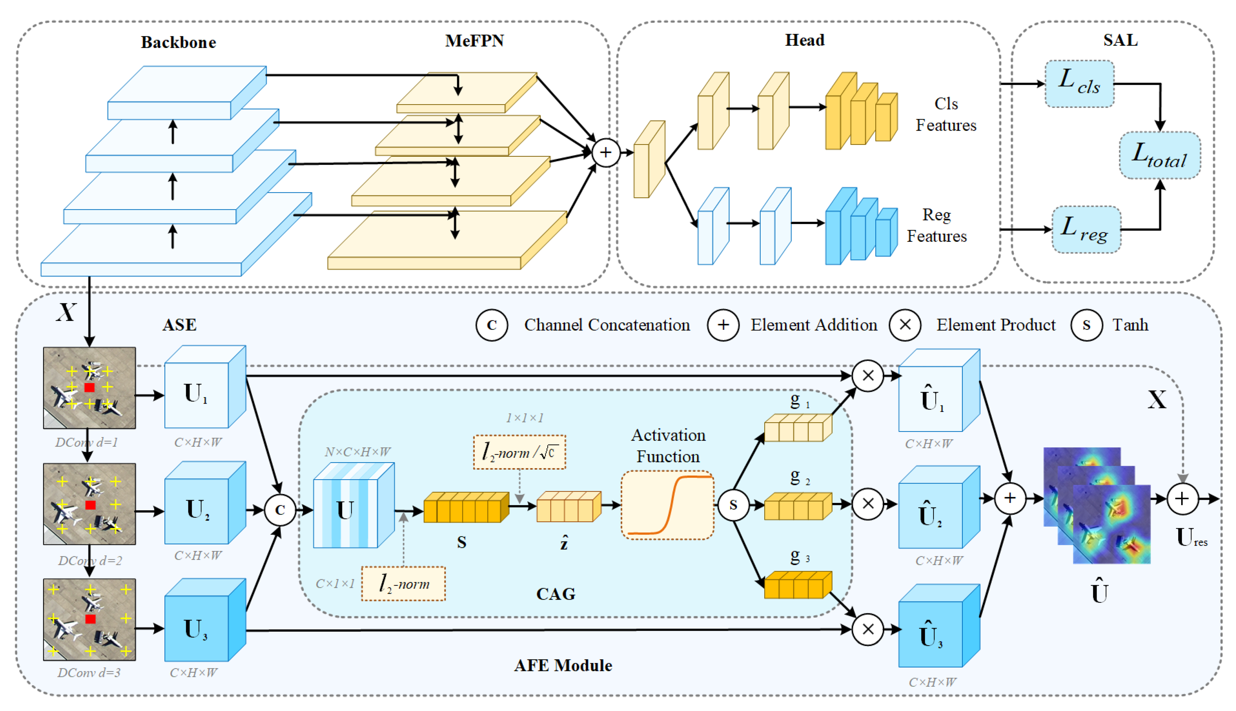
3.1. Adaptive Feature Extraction Module

Traditional object detection methods use fixed-sized convolution kernels and a single network structure. When dealing with objects of different scales, it is difficult for them to adapt to scale changes and they cannot effectively extract comprehensive features.

Parallel Dilated Convolution Sequence: AFE adopts a parallel dilated convolution sequence. This design expands the receptive field without extra parameters and excels in tasks like image recognition requiring a good grasp of data spatial relationships. The pseudocode of this module is shown in

Table 1. AFE algorithm.

Input	x: feature map, $x\in {\mathbb{R}}^{C\times H\times W}$
Output	$\widehat{U}$: enhanced feature map, $\widehat{U}\in {\mathbb{R}}^{C\times H\times W}$
	for each branch in range(branch_count):
	$U=convolution(x,kernels=[1,3,5,7\left]\right)$
	Function L2norm(u, $\alpha$, $ϵ=1e-5$):
	$s\leftarrow$ sum(sum(x**2 for x in row) for row in u)
	$\widehat{s}\leftarrow \alpha \ast (s+ϵ)$ ** 0.5
	return $\widehat{s}$
	for c in range(0, C)
	$\widehat{z}\left[c\right]\leftarrow L2norm\left(U\left[c\right]\right)\times sqrt\left(C\right)/sum(L2norm\left(U\left[c\right]\right)$)
	$g\left[c\right]\leftarrow 1+tanh(\gamma \times \widehat{z}\left[c\right]+\beta )$
	$\widehat{U}\left[c\right]\leftarrow g\left[c\right]\times U\left[c\right]$
	return $\widehat{U}$

. Assume that the input feature map is denoted as $X\in R^{C\times H\times W}$, and the output of each branch can be formulated as follows:

$$U(x,y)=\sum _{i=0}^H\sum _{j=0}^W\left(x+d\times i,y+d\times j\right)·K(i,j)$$

(1)

where d represents the dilation rate, which determines the interval of skipping pixels during the convolution process of the convolutional kernel, and $K(i,j)$ is the kernel function that describes the specific operation rules of the convolution operation.

The receptive fields of different branches can be expressed as

$${\mathrm{RF}}_m=\left\{\begin{array}{cc}(k-1)\times d_m+1,\hfill & \mathrm{if}m=1\hfill \\ {\mathrm{RF}}_{m-1}+(k-1)\times d_m,\hfill & \mathrm{otherwise}\hfill \end{array}\right.$$

(2)

Here, k denotes the kernel size, $R{F}_{m-1}$ stands for the receptive field of the preceding layer, and $d_m$ is the dilation rate of the current layer. The dilation rates of various layers can be configured based on practical requirements. By doing so, the network is able to flexibly modify the size of the receptive field to meet the feature extraction needs of objects at different scales.

All branch outputs are combined in the channel dimension, with the following formula representing this process:

$$U=Concat(U_1,U_2,...,U_n)$$

(3)

where n represents the number of branches, and $Concat$ represents the concatenation operation along the channel. Through this concatenation method, the features with different receptive fields extracted by different branches are fused to obtain more abundant feature information.

Channel Attention Gating Module: Selective kernel network (SKNet) [33] uses global average pooling (GAP) and fully connected layers to perceive the relationships between channels and assign channel importance. However, for normalized inputs, its output lacks discrimination among different samples. Moreover, global average pooling is insensitive to noise and outliers, and these will be averaged into the final result, affecting the model’s stability. To resolve these issues, the present paper employs the normalized CAG. For the features of each branch, the $L_2$-norm [34] is calculated along the channel dimension. Unlike average pooling and max pooling, which select the maximum or average value within the pooling window as output, the $L_2$-norm, computed as ${\parallel \mathbf{x}\parallel }_{L_2}=\sqrt{{\sum }_{i=1}^n{x}_i^2}$, can preserve richer feature information. This enables the extraction of more detailed features during the feature extraction phase. The formula for the $L_2$-norm is as follows:

$$s_c={\alpha }_c·{\parallel u_c\parallel }_{L_2}={\alpha }_c·{\left\{\left[\sum _{i=0}^H\sum _{j=1}^W{\left(u_c^{i,j}\right)}^2\right]+ϵ\right\}}^{{\displaystyle \frac{1}{2}}}$$

(4)

Here, ${\alpha }_c$ is a learnable weight parameter used to adjust the importance of each channel’s feature, and $ϵ$ is assigned a value of ${10}^{-5}$ to prevent division-by-zero errors during the computation.

The feature vector of each channel is processed through a parameter-free normalization technique based on $L_2$-norm scaling, and the formula is as follows:

$${\widehat{z}}_c={\displaystyle \frac{\sqrt{C}{s}_c}{{\parallel S\parallel }_{L_2}}}={\displaystyle \frac{\sqrt{C}{s}_c}{{\left[\left({\sum }_{c=1}^C{s}_c^2\right)+ϵ\right]}^{\frac{1}{2}}}}$$

(5)

The scalar $\sqrt{C}$ is introduced to adjust the scale of ${\widehat{z}}_c$, preventing its value from being too small when the number of channels C is large, and ensuring the comparability of features of different channels in subsequent calculations. Subsequently, the activation function $tanh$ is used to dynamically adjust the contribution of features, and the formula is

$${\widehat{\mathrm{u}}}_{\mathrm{c}}={\mathrm{u}}_{\mathrm{c}}·[1+tanh({\gamma }_{\mathrm{c}}·{\widehat{\mathrm{z}}}_{\mathrm{c}}+{\beta }_{\mathrm{c}})]$$

(6)

Here, ${\widehat{s}}_c$ represents the normalized scale vector, while ${\gamma }_c$ and ${\beta }_c$ denote the gating weight and bias, respectively. These are employed to adaptively regulate the scale of each channel within the feature map. The output of the $tanh$ function lies within the range of $[-1,1]$. This property can effectively preserve numerical stability throughout the training process and permits the adjustment of feature contributions in both positive and negative directions. As a result, the model can better adapt to diverse feature distributions.

3.2. Multi-Scale Enhanced Feature Pyramid Network

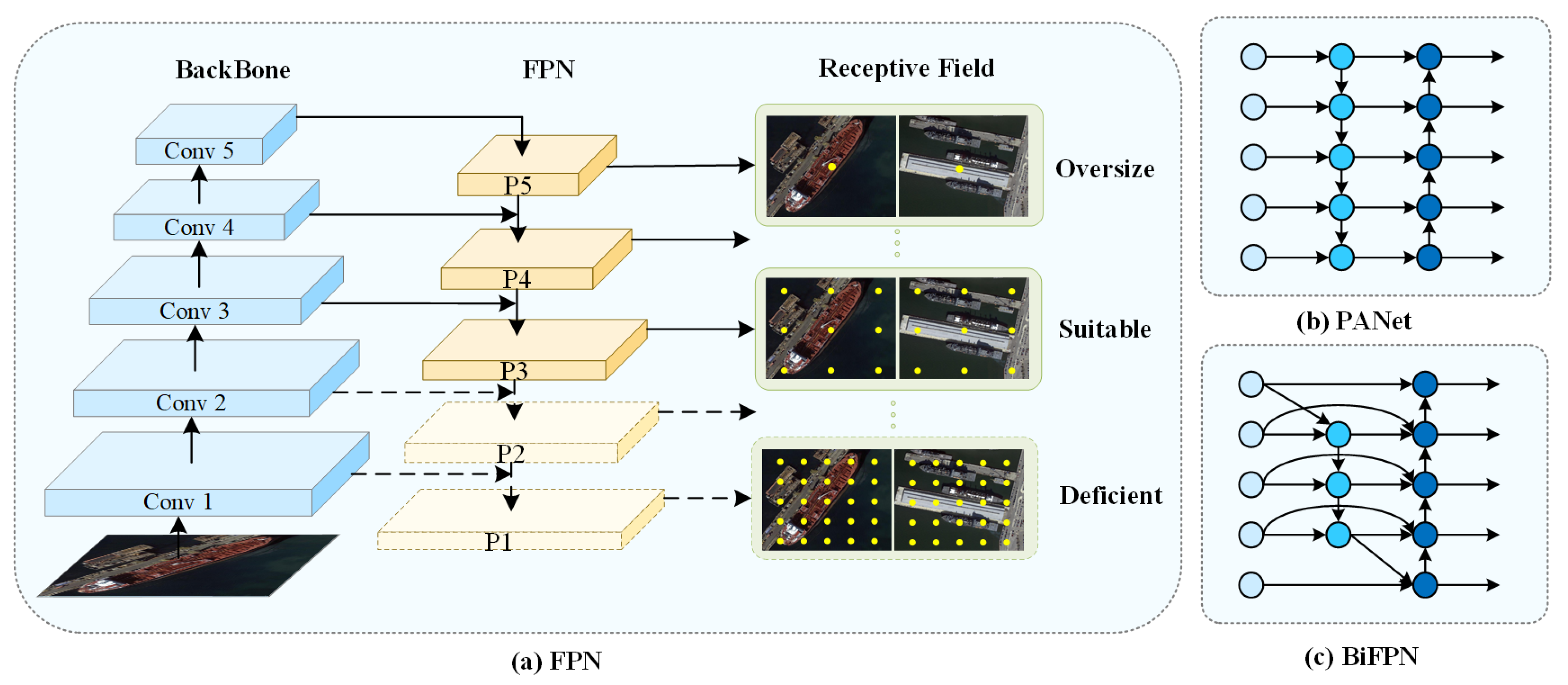
Previously, in the realm of feature fusion, numerous methodologies frequently resorted to straightforward techniques like feature concatenation or direct addition to integrate multi-level features, as depicted in Figure 3b. This approach overlooks the disparities in scale and semantics among features at various levels. Consequently, it readily leads to information loss or semantic ambiguity in the fused features, making it arduous to fully harness the merits of features at each layer during object detection.

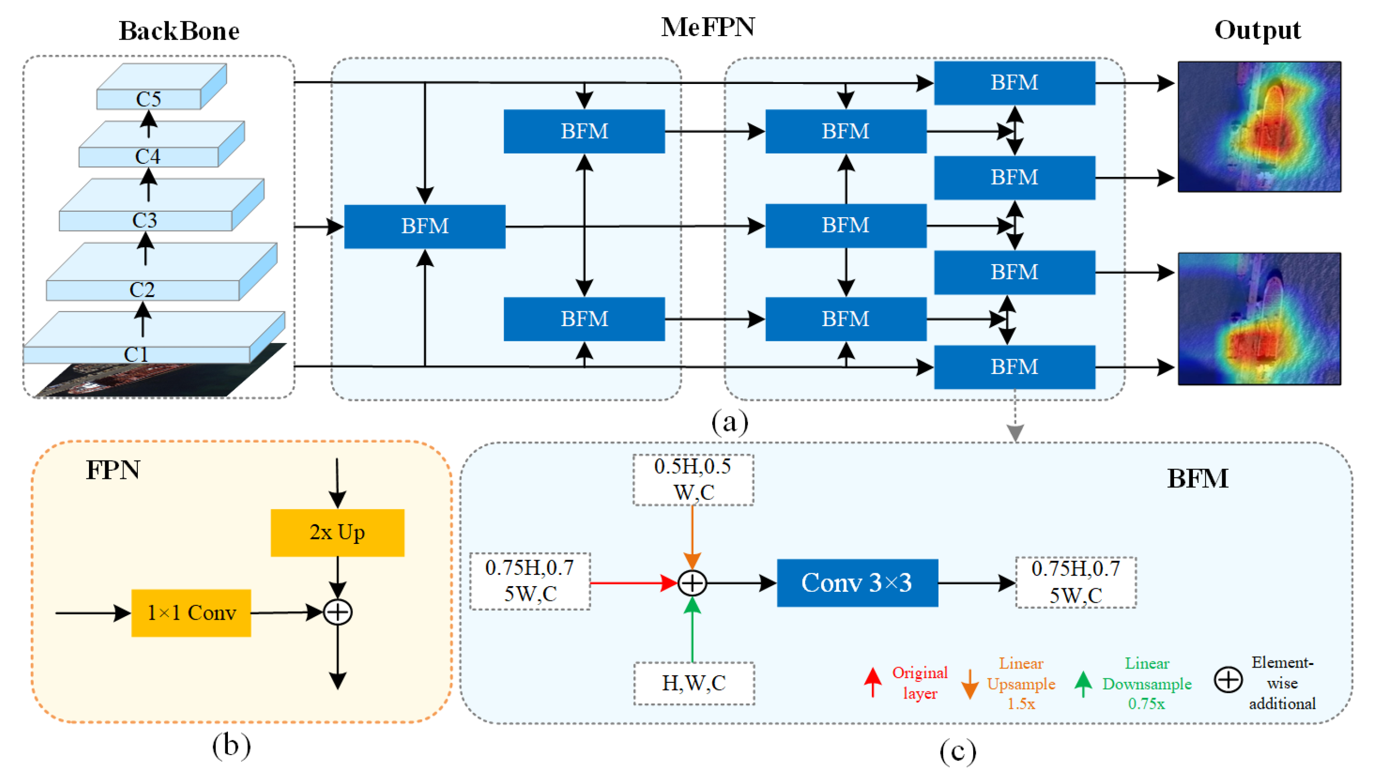
To effectively utilize multi-level features, MeFPN integrates a BFM based on structural symmetry, as illustrated in Figure 3a. Within the BFM (Figure 3c), a linear scale transformation is applied to align features from different levels to a common intermediate scale. This ensures that features from various levels can be fused at a unified scale, facilitating the efficient integration of high-level semantic cues with low-level fine-grained details. The formula for linear scale transformation is as follows:

$$F_{up}=UpSampling(F_{high},\psi )$$

(7)

$$F_{down}=DownSampling(X_{low},\varphi )$$

(8)

Here, $\psi$ and $\varphi$ represent the scaling factors for upsampling and downsampling, respectively. We employ bilinear interpolation to upscale higher-level feature maps, bringing their scales closer to the intermediate level in upsampling.The upsampling factor $\psi =1.5$, and the new pixel value is computed as a weighted average of four neighboring pixels:

$$F_{\mathrm{up}}(i,j)=\sum _{m=0}^1\sum _{n=0}^1{w}_{mn}·F_{\mathrm{high}}\left(⌊{\displaystyle \frac{i}{\psi }}⌋+m,⌊{\displaystyle \frac{j}{\psi }}⌋+n\right)$$

(9)

Here, $F_{up}$ is the upsampled feature map, $w_{mn}$ denotes the weight coefficient determined by the relative position of the new coordinate $(i,j)$ and neighboring pixels, and $F_{high}$ represents the pixel values in the higher-level feature map.

We employ convolution-based downsampling with a fixed stride to adjust lower-level feature maps. Specifically, a convolution kernel slides over the lower-level feature map with a downsampling factor $\varphi =0.75$, following the equation

$$F_{\mathrm{down}}(i,j)=\sum _{m=0}^{k-1}\sum _{n=0}^{k-1}K(m,n)·F_{\mathrm{low}}(i·s+m,j·s+n)$$

(10)

Here, $F_{down}$ is the downsampled feature map, K represents the convolution kernel value at position $(m,n)$, $F_{low}$ denotes the corresponding pixel value in the original lower-level feature map, and k is the kernel size. The stride s is determined by the downsampling factor $\varphi$.

To enhance the feature representation, the scaled features are combined with the original layer features in an element-wise manner. The corresponding formula is presented below:

$$F_{add}=F_{orig}+F_{up}+F_{down}$$

(11)

where $F_{orig}$ represents the features of the original layer. This preserves the advantages of each layer while enriching the overall feature set.

Finally, further feature extraction and fusion are carried out through a convolution operation to achieve more in-depth feature extraction. The formula for the fusion layer is

$$F_{fused}=Conv(F_{add},K)$$

(12)

Here, K is a $3\times 3$ convolution kernel, and $Conv$ the convolution operation. The convolution screens and integrates fused features to extract more representative ones, boosting the model’s multi-scale object detection ability.

Therefore, the BFM design of MeFPN not only maintains high-efficiency feature fusion but also enhances the feature representation and discriminative ability through precise scale alignment and a two-way fusion mechanism. It achieves more flexible and accurate feature capture of multi-scale objects with lower computational complexity. The pseudocode of it is shown in

Table 2. MeFPN algorithm.

Input	x: feature map, $x\in {\mathbb{R}}^{C\times H\times W}$
Output	F: enhanced feature map, $F\in {\mathbb{R}}^{C\times H\times W}$
	for index in range(1,n+1)
	Higher-level feature map $F_{high}$, Upsampling scale factor $\psi =1.5$
	$F_{up}\leftarrow \mathrm{Bilinear}\mathrm{interpolation}(F_{high},\mathrm{scale}\mathrm{ratio}=\psi )$
	Lower-level feature map $F_{low}$, Downsampling scale factor $\varphi =0.75$
	$F_{down}\leftarrow \mathrm{convolution}(F_{low},K=k_{down},\mathrm{stride}=s_{down})$
	Combine feature maps $F_{add}=F_{orig}+F_{up}+F_{down}$
	Fusion convolution $F_{fused}\leftarrow \mathrm{convolution}(F_{add},K)$
	return $F_{fused}$

. By stacking multiple BFMs, features at different levels can be combined more fully, further enhancing the feature representation ability.

3.3. Scale-Aware Loss Function

In remote sensing images, detection difficulty varies greatly by object scale. Small objects are harder to detect due to small pixel proportion and vague features [35]. Traditional loss functions treat all-scale objects alike when computing losses, causing the network to struggle to improve small-object detection accuracy during training and thus affecting overall performance.

To balance detection difficulty differences, we introduce a scale-sensitive loss function that adjusts loss weights by object scale. Specifically, a scale weight ${\delta }_i$ is added to the classification loss function:

$${\delta }_i={\displaystyle \frac{1}{1+{\mathrm{e}}^{-\rho (s_i-\mu )}}}$$

(13)

Here, the relative scale of an object is given by $s_i=\sqrt[2]{{\displaystyle \frac{w_{gt}\times h_{gt}}{W_i\times H_i}}}$, where $w_{gt}$, $h_{gt}$, $W_i$, and $H_i$ are object and image width-height values, respectively. Trainable parameters $\rho$ and $\mu$ are vital for regulating adjustment speed and maintaining scale-weight balance. Their values generally range for $\rho$ from $0.1$ to 10 (increased for datasets with many small objects), and $\mu$ is selected around the average relative scale $s_{avg}$ based on target scale statistics. In actual training, random initialization and gradient descent are combined to fine tune them. In the DOTA [36] dataset experiment, with dense small objects, multiple comparative tests show the model performs well when $\rho =5$ and $\mu =0.1$. The classification loss function is expressed as

$$Los{s}_{cl{s}_{-}scale}=-{\delta }_i·\alpha ·{(1-\widehat{y})}^b·log\left(\widehat{y}\right)$$

(14)

Here, $\alpha$ is a balance factor for sample balancing, adjusting sample weights in loss calculation, and $\widehat{y}$ is the model’s predicted probability. The focusing parameter b is usually 2, reducing the loss weight of easy-to-classify samples so the model focuses on hard-to-classify ones. For small objects, ${\delta }_i$ is small, increasing classification loss and making the model focus on them. For large objects, ${\delta }_i$ is near 1, with no obvious increase in classification loss, ensuring stable detection.

The intersection over union (IoU) [37] is commonly employed as a metric for evaluating regression loss. Nevertheless, IoU comes with certain limitations. Take the situation where there is no overlap between the ground-truth box (GT) and the anchor box, for instance; in such a case, the IoU value drops to 0, potentially resulting in the vanishing gradient problem. Moreover, when the anchor box is entirely enclosed within the GT box, IoU fails to precisely assess the positioning status.

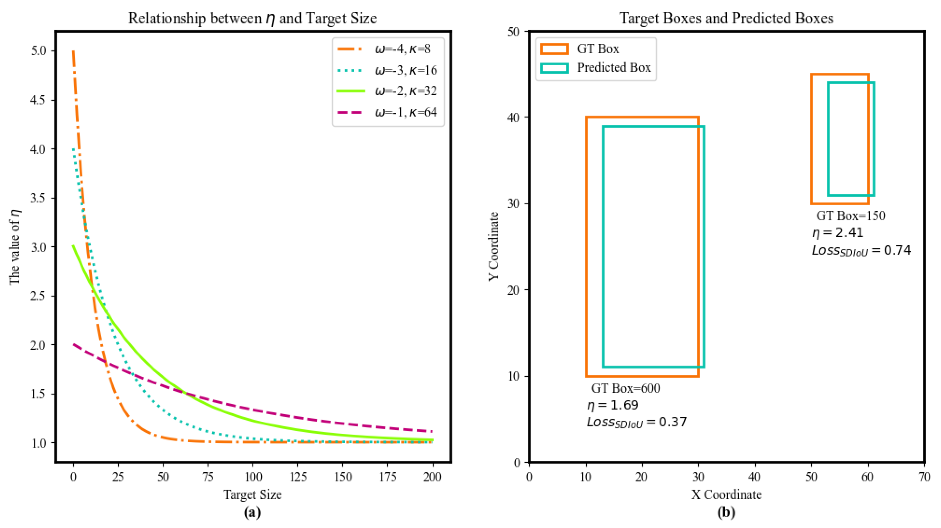
To address these issues, this paper proposes the scale-aware intersection over union (SDIoU), which balances the loss contribution of objects of different sizes through the scale weight $\eta$. As shown in Figure 4, the GT box is $B_{gt}=(x_{gt},y_{gt},w_{gt},h_{gt})$ and the anchor box is $B_p=(x_p,y_p,w_p,h_p)$. The SDIoU is defined as follows:

$$Los{s}_{SDIoU}=1-IO{U}^{\eta }-{\displaystyle \frac{d^2}{c^2}}$$

(15)

$$\eta =1-\omega ·exp\left(-{\displaystyle \frac{\sqrt{w_{gt}{h}_{gt}+w_p{h}_p}}{\sqrt{2}\kappa }}\right)$$

(16)

Here, d is the Euclidean distance between the GT box and anchor box centers, c is the diagonal of their smallest enclosing box, $\eta$ is the scale weight, $\omega \in (-\infty ,1]$ adjusts small-object scaling, and $\kappa$ determines large-object’s return rate to standard IoU. Multiple tests show the model gets best accuracy for different-scale objects when $\omega =-3$ and $\kappa =16$. In practice, these two parameters are fine tuned based on dataset features and task requirements.

The SAL integrates the $Los{s}_{cl{s}_{-}scale}$ and the $Los{s}_{SDIoU}$ to formulate an overall loss function:

$$Los{s}_{total}={\rho }_{cls}{\displaystyle \frac{1}{M}}\sum _{i=1}^{M}Los{s}_{cl{s}_{-}scale}+{\lambda }_{reg}{\displaystyle \frac{1}{N}}\sum _{i=1}^{N}Los{s}_{SDIoU}$$

(17)

where ${\rho }_{cls}$ and ${\lambda }_{reg}$ are the weights of the classification and regression error terms, respectively. In the experiments, their values are set to ${\rho }_{cls}=0.7$ and ${\lambda }_{reg}=0.3$. The determination of these two weights is obtained through comparative experiments on multiple datasets, comprehensively considering indicators such as the precision and recall rate of the model in the detection of objects at different scales. By using scale-reciprocal loss weighting in the SAL function, these symmetric components collectively enhance the system’s robustness to scale variations while maintaining computational efficiency.

4. Experimental Methods and Discussion

4.1. Experimental Details

(1) Experimental Environment: The experiment was conducted on a system equipped with eight NVIDIA GeForce RTX 4090D GPUs for computational support; the experimental code was developed based on the MMRotate [38] framework built on PyTorch 1.13.1, providing convenient tools and efficient implementations.

(2) Selection of Backbone Networks: ResNet50 and ResNet101 [39] were selected as backbone networks. The baseline model used was $R^{3}Det$ [19], a single-stage rotated object detector, which performs exceptionally well in detecting rotated objects with high aspect ratios. This model serves as a reliable reference for evaluating AFEDet’s performance.

(3) Data Processing: The DOTA dataset has a high resolution, and input images were cropped into 1024 × 1024 pixel blocks. To prevent information loss and enhance data diversity, a sliding window with a 200-pixel overlap was applied. For HRSC2016 [40] and UCAS-AOD [41] datasets, images were resized to 512 × 800 pixels [42]. The data augmentation included random horizontal, vertical, or diagonal flipping (25% probability), and random rotation (50% probability).

(4) Training Parameter Settings: For the DOTA dataset, training and validation sets were merged. The AdamW optimizer was used with a batch size of 32, the initial learning rate $lr$ was $1\times {10}^{-4}$, momentum was set among $[9\times {10}^{-1},9.99\times {10}^{-1}]$, and the weight decay was $5\times {10}^{-2}$. Training was for 24 epochs, with the $lr$ linearly decaying from epoch 16 to epoch 22. For the HRSC2016 and UCAS-AOD datasets, training and validation sets were also merged. The SGD optimizer was used with a batch size of 32, an initial learning rate $lr=5\times {10}^{-3}$, momentum of $9\times {10}^{-1}$, and a weight decay of $1\times {10}^{-4}$. Training was for 36 epochs, with the learning rate decaying from epoch 24 to epoch 33.

4.2. Datasets

(1) DOTA [36]: a large-scale remote sensing object detection dataset with 15 categories, including buildings, vehicles, and other common objects. This dataset contains 2806 images with resolutions ranging from 800 × 800 to 4000 × 4000 pixels, simulating various imaging conditions. It also includes over 188,000 annotated object instances, providing a rich resource for model training, facilitating precise object recognition and localization.

(2) HRSC2016 [40]: extracted from Google Earth images, this dataset contains 27 categories and is specifically designed for ship detection; oriented bounding box (OBB) annotations are used for precise ship localization. This dataset contains 1061 labeled images, with 436 for training, 181 for validation, and 444 for testing.

(3) UCAS-AOD [41]: composed of 2127 annotated images collected from Google Earth, this dataset was used primarily for detecting airplanes in various flight states. The image sizes range from 400 × 400 to 1200 × 1200 pixels, and OBB annotations are provided for accurate target localization.

4.3. Evaluation Metrics

To comprehensively evaluate the detection performance of the model, this study adopts precision, recall, mAP, and FPS as evaluation metrics. The mAP represents the average area under the precision–recall curve across different target categories. Precision is the proportion of true positives among all samples predicted as positive, calculated as

$$Precision={\displaystyle \frac{TP}{TP+FP}}$$

(18)

where $TP$ (true positives) represents the correctly predicted positive samples, and $FP$ (false positives) represents the incorrectly predicted positive samples.

Recall measures the proportion of correctly predicted positive samples among all actual positive samples. The calculation formula is as follows:

$$Recall={\displaystyle \frac{TP}{TP+FN}}$$

(19)

where $FN$ (false negatives) represents the actual positive samples that were incorrectly predicted as negative.

The $mAP$ reflects the model’s overall detection performance across all categories. The calculation formula is as follows:

$$mAP={\displaystyle \frac{1}{N}}\sum _{i=1}^{N}A{P}_i$$

(20)

Here, N represents the total number of object categories, and $A{P}_i$ represents the average precision ($AP$) of category i.

4.4. Comparative Experiments

To verify AFEDet’s performance and generalization ability, experiments were conducted on the three public datasets above, comparing AFEDet with state-of-the-art models.

4.4.1. Evaluation on the DOTA Dataset

Table 3. Comparison of AFEDet with state-of-the-art object detection models on the DOTA dataset.

Method	Backbone	mAP (%)	AP (%) for Various Targets
			SV	LV	ST	PL	HA	BD	SH	TC	BR	RA	SP	BC	HC	GTF	SBF
One-stage
$R^{3}Det$ [19]	ResNet101	73.79	76.23	80.39	83.24	88.76	66.91	83.09	86.72	90.78	50.91	61.35	70.63	84.68	53.94	67.27	61.98
FMSSD [43]	ResNet101	72.43	69.23	73.56	73.33	89.11	72.37	81.51	76.87	90.71	48.22	67.52	80.57	82.67	60.15	67.94	52.65
$S^{2}ANet$ [44]	ResNet50	79.42	79.94	83.19	87.81	88.89	78.30	83.60	89.11	90.78	57.74	68.25	77.01	84.87	69.58	81.95	70.30
Two-stage
SCRDet [45]	ResNet101	72.61	68.36	60.32	86.86	89.98	66.25	80.65	72.41	90.85	52.09	66.68	68.24	87.94	65.21	68.36	65.02
DRN [13]	CenterNet	73.23	76.22	74.43	84.89	89.71	89.71	82.34	82.34	82.34	47.22	61.93	69.63	86.18	58.48	64.10	57.65
RoI Trans [20]	ResNet101	75.57	68.81	73.68	81.46	88.64	62.83	78.52	83.59	90.74	43.44	53.54	58.93	77.27	47.67	75.92	58.39
SCRDet++ [46]	ResNet101	76.24	69.62	81.17	85.10	90.01	77.69	82.32	78.83	90.86	61.94	61.12	80.68	86.32	64.25	68.62	65.10
NPMMRDet [12]	ResNet101	76.16	76.93	84.08	86.32	89.44	79.61	83.18	88.25	90.87	54.50	68.16	79.51	88.29	57.26	66.10	49.95
DAL [47]	ResNet50	76.90	81.90	88.46	64.41	83.11	72.09	55.03	90.89	84.97	71.00	65.65	72.09	87.46	64.35	78.30	65.65
DCL [18]	ResNet152	77.37	82.56	87.31	67.49	83.60	70.56	53.54	90.67	86.59	72.76	73.29	70.56	86.98	69.99	79.04	66.88
G-Rep [48]	ResNet101	80.16	80.94	85.68	87.77	88.15	77.19	81.64	88.37	90.90	61.30	67.42	81.23	85.47	75.83	79.50	71.01
ReDet [49]	ResNet50	80.10	78.34	86.06	87.03	88.81	79.26	82.48	88.31	90.87	60.83	66.90	79.71	88.77	74.67	80.82	68.65
AFEDet (Ours)	ResNet101	80.91	79.70	81.12	72.15	81.66	80.96	81.51	81.12	81.73	77.96	81.66	80.87	88.75	81.66	81.51	81.38

presents the evaluation results on the DOTA dataset. AFEDet achieved an mAP of 80.91%, outperforming all comparison methods. Compared with similar methods, mAP improved by 7.12% over a baseline model, and mAP increased by 8.48% compared to FMSSD. Even compared to high-performing models, AFEDet still achieved a 1.49% improvement.

For two-stage detection models, AFEDet surpassed G-Rep, SCRDet, and SCRDet++, demonstrating superior detection capabilities in complex remote sensing scenes. For specific categories, small-object detection (PL and HC categories) achieved 81.66% accuracy, surpassing all competing methods. This highlights AFEDet’s ability to capture fine details, which is crucial for accurately detecting small targets in real-world applications.

4.4.2. Evaluation on the HRSC2016 Dataset

The evaluation results on the HRSC2016 dataset are presented in

Table 4. Comparison of AFEDet with state-of-the-art object detection models on the HRSC2016 dataset.

Method	Backbone	mAP (%)	FPS
$R^{2}CNN$ [21]	ResNet101	73.07	2.00
DCL [18]	ResNet101	89.46	-
TIOE-Det [50]	ResNet101	90.16	-
$S^{2}ANet$ [44]	ResNet101	90.17	12.70
Oriented RCNN [51]	ResNet101	90.50	15.10
$R^{3}Det$ [19]	ResNet101	89.26	20.00
AFEDet (Ours)	ResNet101	91.88	22.90

. When AFEDet was implemented with ResNet101 as the backbone network, it achieved an mAP of 91.88%, significantly outperforming many comparison methods. In terms of accuracy improvement, AFEDet showed remarkable gains compared to other models. Specifically, it outperformed $R^{2}CNN$ by 18.81%, achieved an increase of 2.42% over DCL, and demonstrated an improvement of 1.72% over TIOE-Det. When compared to $S^{2}ANet$ and $R^{3}Det$, the model’s performance improved by 1.71% and 2.62%, respectively. Even when compared to Oriented RCNN, which achieved an mAP of 90.50%, AFEDet still maintained an accuracy advantage, further confirming its effectiveness in remote sensing object detection.

Regarding FPS performance, AFEDet demonstrated outstanding efficiency, achieving 22.9 FPS, which is significantly higher than $R^{2}CNN$ (2.0 FPS) and $R^{3}Det$ (12.0 FPS). Although $S^{2}ANet$ and Oriented RCNN achieved 12.7 FPS and 15.1 FPS, respectively, AFEDet maintained a higher mAP while offering superior detection speed. This balance between high detection accuracy and fast processing speed highlights AFEDet’s practical potential.

4.4.3. Evaluation on the UCAS-AOD Dataset

For the UCAS-AOD dataset, we conducted experiments using ResNet50 as the backbone network to evaluate the detection performance of AFEDet. The results, presented in

Table 5. Comparison of AFEDet with state-of-the-art object detection methods on the UCAS-AOD dataset.

Method	Backbone	Car (AP%)	Airplane (AP%)	mAP (%)
R-RetinaNet [52]	ResNet50	84.64	90.51	87.57
FasterRCNN [53]	ResNet50	86.87	89.86	88.36
RoI Transformer [20]	ResNet50	88.02	90.02	89.20
G-rep [48]	ResNet50	89.64	90.30	90.16
DAL [47]	ResNet50	89.25	90.49	89.87
$S^{2}ANet$ [44]	ResNet50	89.56	90.42	89.99
$R^{3}Det$ [19]	ResNet50	89.65	89.89	89.42
AFEDet (Ours)	ResNet50	90.30	90.46	90.28

, indicate that AFEDet achieved an mAP of 90.30%, demonstrating its strong capability in remote sensing object detection. Breaking down the results further, AFEDet obtained an AP of 90.46% for vehicle detection and 90.28% for airplane detection, outperforming other methods in both categories. Compared to R-RetinaNet, AFEDet achieved a 2.73% improvement in mAP, while it outperformed Faster R-CNN by 1.94%. In comparison with RoI Transformer, AFEDet still demonstrated a 1.1% advantage in detection accuracy. Even when evaluated against competitive models such as G-Rep, DAL, and $S^{2}ANet$, AFEDet consistently achieved the highest mAP, further solidifying its superior performance in object detection tasks. These results confirm that AFEDet exhibits strong target detection capabilities on the UCAS-AOD dataset, excelling in both precision and localization accuracy.

4.4.4. Detection Visualization Results

(1) The Visualization Result of DOTA

In Figure 5a,b, both large and medium-sized objects can be easily and accurately identified. Even for elongated targets, as shown in Figure 5c–e, precise recognition can still be achieved. In Figure 5k–o, various densely parked targets, such as airplanes and ships, are also accurately detected. Figure 5f–j present the prediction results of objects of different sizes and shapes in a complex background. Notably, in Figure 5n, objects of varying sizes have been successfully detected.

(2) The Visualization Result of HRSC2016

Figure 6 presents detection results on the HRSC2016 dataset, where AFEDet demonstrates highly efficient detection performance. As shown in Figure 6a,c, the model accurately detects various types of ships densely docked in ports, including large cargo ships and small warships. The bounding boxes tightly fit the ship contours, emphasizing the model’s precision in target localization. Even in complex backgrounds, as illustrated in Figure 6d–f, AFEDet successfully differentiates individual ships, effectively reducing missed detections. The ability to distinguish ships even in cluttered and densely populated harbor environments highlights the robustness and accuracy of AFEDet’s detection mechanism.

(3) The Visualization Result of UCAS-AOD

Figure 7 displays detection results on the UCAS-AOD dataset, further demonstrating AFEDet’s adaptability in various scenarios. As shown in Figure 7a, the model achieves high-precision airplane detection, ensuring tight bounding box alignment, even for small and distant aircraft. In densely packed parking areas, AFEDet effectively differentiates each airplane, minimizing overlapping bounding boxes and avoiding false detections. Additionally, Figure 7b illustrates detection results in urban road environments, where AFEDet maintains strong performance despite background interference from buildings, vegetation, and other structures. The model’s ability to accurately detect vehicles of various sizes and orientations further underscores its robustness in complex backgrounds.

(4) Detection Results under Extreme Lighting Variations

As shown in Figure 8, the model demonstrates stable detection performance under extreme lighting variations. Even in low-light environments where object features are barely visible, such as in Figure 8e,g, the model is still capable of recognizing small objects that are difficult to detect with the naked eye, showcasing strong robustness in challenging conditions.

4.5. Ablation Study

4.5.1. Key Component Analysis

To further analyze the impact of different modules on the performance of AFEDet, we conducted an ablation study using the DOTA dataset. The results, presented in

Table 6. Ablation study results of AFEDet.

Method	Backbone	mAP (%)	Recall (%)	Precision (%)
Baseline	ResNet-50	84.68	83.61	82.82
Baseline+AFE	ResNet-50	87.59	88.12	86.42
Baseline+MeFPN	ResNet-50	88.90	88.34	88.21
Baseline+SAL	ResNet-50	86.27	87.41	85.13
AFEDet (Ours)	ResNet-50	91.29	91.50	90.89

, show that each module contributes significantly to the overall performance of the model. The baseline model, which lacks the AFE, MeFPN, and SAL modules, achieved an mAP of 84.68%. When AFE was added, the mAP increased to 87.59%, reflecting an improvement of 3.44%. Additionally, recall and precision saw improvements of 5.3% and 4.34%, respectively. This indicates that AFE effectively enhances multi-scale feature extraction through parallel dilated convolution and channel attention mechanisms, significantly improving detection accuracy. Integrating MeFPN further boosted the mAP to 88.90%, representing an additional improvement of 4.98% compared to the baseline. This performance gain can be attributed to MeFPN’s bidirectional fusion strategy, which enhances feature alignment across different scales, reduces feature degradation, and improves information retention. Furthermore, incorporating the SAL function resulted in an mAP increase to 86.27%, an improvement of 1.88% over the baseline. The SAL function optimizes loss balancing for small-object detection, increasing the model’s ability to capture and accurately recognize small-scale targets.

When all three modules-AFE, MeFPN, and SAL-were combined, AFEDet achieved its highest mAP of 91.29% (7.8%↑), with recall improving by 9.4% and precision increasing by 9.7% compared to the baseline. These results confirm that the integration of these three modules significantly enhances AFEDet’s ability to detect multi-scale objects, making it more effective in complex remote sensing scenarios.

The visualization results in Figure 9 indicate that AFE enhances feature extraction by making feature representation more focused and highlighting key information. MeFPN improves the model’s response accuracy to multi-scale targets. After integrating these three modules, AFEDet achieves the most precise response in the target regions, demonstrating strong object localization capabilities.

4.5.2. Parameter Analysis of SDIoU

To investigate the impact of SDIoU parameters on the model’s performance in detecting objects of different scales, we conducted an ablation study using the DOTA dataset. The detailed experimental results are shown in

Table 7. Comparison of different loss functions’ performance on object detection.

Loss Function	Parameters	mAP (%)	S (P)	S (R)	M (P)	M (R)	L (P)	L (R)
IoU	-	77.30	74.10	65.50	78.30	75.20	79.70	82.40
DIoU	-	78.50	75.40	70.20	79.80	76.90	80.30	83.10
SDIoU	$\gamma =-1,\kappa =64$	78.90	76.80	72.00	79.60	76.50	80.50	83.50
SDIoU	$\gamma =-2,\kappa =32$	79.40	77.10	73.10	80.10	77.80	81.20	84.20
SDIoU	$\gamma =-3,\kappa =16$	80.80	78.80	75.30	81.50	79.60	82.10	85.40

mAP represents mean average precision, P denotes precision, and R represents recall.

.

In this experiment, we adjusted the parameters $\gamma$ and $\kappa$ to observe changes in the model’s sensitivity and accuracy for different target scales. To determine the optimal values for $\gamma$ and $\kappa$, we first referred to the weight formula $\eta =1-\omega ·exp\left(-{\displaystyle \frac{\sqrt{w_{\mathrm{gt}}{h}_{\mathrm{gt}}+w_{\mathrm{p}}{h}_{\mathrm{p}}}}{\sqrt{2\kappa }}}\right)$, combined with the model’s theoretical principles and prior research experience, to preliminarily define the parameter ranges as $\gamma =[-5,5]$ and $\kappa$ = [1, 64]. Next, we selected multiple parameter combinations within the defined range and employed a five-fold cross-validation method to precisely record key performance metrics, including detection precision and recall for small, medium, and large targets. Simultaneously, we monitored the effect of variations in $\gamma$ and $\kappa$ on $\eta$ and overall model performance.

Through extensive experimentation and data analysis, we found that reducing the values of $\gamma$ and $\kappa$ significantly improved the model’s localization sensitivity for small targets, leading to a substantial increase in small-target detection accuracy. As shown in Table 7, when $\gamma$ and $\kappa$ were set to relatively small values (e.g. $\gamma =-3,\kappa =16$), the model achieved a mAP of 80.8% (an improvement of 3.5%), while the detection accuracy for small targets (column S) increased to 78.8% (a 4.7% improvement). This enhancement is particularly significant compared to traditional IoU and DIoU methods, which do not incorporate scale adaptivity, strongly validating the effectiveness of SDIoU in small-object detection. Based on a comprehensive evaluation of the model’s performance across different target scales, we determined the optimal values of $\gamma$ and $\kappa$, ensuring the model achieves the highest possible accuracy when detecting objects of varying scales.

4.5.3. Computational Complexity Analysis

To evaluate the practicality of the proposed method in real-world applications, we compare different object detection models in terms of parameter count, floating-point operations (FLOPs), and FPS. The results are shown in

Table 8. Comparison of different remote sensing object detection models in terms of parameters, FLOPs, and FPS.

Model	Params (M)	FLOPs (G)	FPS
$R^{3}Det$ [19]	38.54	196.21	8.3
SKNet-101 [33]	48.9	8.46	–
LSKNet [30]	31.0	161.0	20.5
MSRO-Net [28]	42.98	168.09	12.5
AFENet (ours)	20.91	50.26	19.7

.

AFEDet demonstrates a significant advantage in parameter efficiency, with only 20.91M parameters, considerably lower than models like LSKNet (31.0M). This compact parameter design reduces storage requirements and memory consumption, enhancing deployability on resource-constrained devices. In terms of computational complexity, AFEDet achieves 50.26G FLOPs, which is lower than most comparison models, indicating its ability to operate efficiently under limited computational resources while maintaining detection accuracy. AFEDet achieves 19.7 FPS, outperforming $R^{3}Det$ (8.3 FPS) and MSRO-Net (12.5 FPS) and approaching LSKNet (20.5 FPS). This demonstrates that AFEDet effectively balances detection speed and computational cost, meeting real-time processing requirements. The improvements in inference speed can be attributed to the parameter-free normalization method and the BFM, which enable precise alignment of intermediate-layer features and accelerate information flow within the model.

In comparison, MSRO-Net has a high parameter count and FLOPs, resulting in increased computational complexity and limiting its scalability. Although SKNet-101 has lower FLOPs, its higher parameter count may introduce additional challenges. Overall, AFEDet achieves a well-balanced trade-off between parameters, computational cost, and speed, enabling efficient detection with low complexity. This makes AFEDet a cost-effective solution for remote sensing object detection with strong practical applicability.

5. Discussion of Experimental Results

The ablation study demonstrates that the three key modules AFE, MeFPN, and SAL effectively enhance the performance of AFEDet. AFE leverages parallel dilated convolutions and channel attention mechanisms to improve the model’s adaptability to multi-scale targets. MeFPN reduces information loss and enhances feature perception through bidirectional fusion strategies. The SAL function optimizes small-object detection, improving both model accuracy and robustness. The synergy among these modules enables AFEDet to excel in multi-scale object detection and achieve outstanding results across multiple remote sensing datasets.

However, AFEDet still faces certain challenges. As illustrated in Figure 10, the model struggles to detect densely packed or overlapping objects. Most existing algorithms primarily focus on individual object features, making it difficult for the model to recognize occluded object boundaries, leading to missed detections. Future research will explore semantic segmentation techniques to distinguish occluded and visible parts, thereby enhancing the model’s ability to extract features from occluded areas and guiding it to uncover potential hidden features. For large-scale objects, as depicted in Figure 11, the model faces challenges due to image cropping. When a large object is divided into multiple image patches, the model learns only the segmented parts rather than the entire object structure. This discrepancy between the segmented features and the original complete feature distribution results in detection difficulties. To address this issue, we plan to incorporate ViT [54] (Vision Transformer) architectures to capture long-range dependencies, helping the model understand the complete structure of large objects.

Overall, while AFEDet focuses on addressing object scale diversity, it still faces limitations in handling occluded targets, complex object appearances, and extreme variations in real-world scenarios. The sample balancing process is insufficient, leading to under-representation of certain complex scenarios, while data augmentation techniques remain relatively simple. Future improvements should focus on optimizing these aspects to further enhance model performance.

6. Conclusions

The proposed AFEDet aims to achieve an optimal balance between multi-scale feature extraction and computational complexity. By incorporating a channel attention mechanism, an $L_2$-norm-based gating module, a bidirectional fusion module, and a dynamic weight adjustment loss function, AFEDet has demonstrated outstanding performance across multiple remote sensing datasets, with the effectiveness of its key components validated through ablation experiments. However, challenges remain in handling occluded and extremely large objects; also, further improvement in computational speed for real-time applications is expected. Future research will explore ViT [54] or multi-head attention mechanisms, model distillation, and pruning techniques to enhance both accuracy and efficiency. Additionally, we plan to extend AFEDet to applications in low-altitude flight [1] and field exploration [2], with targeted optimizations to improve its robustness and adaptability across diverse scenarios.