Abstract
We compared two methods for determining the detector performance and the cosmic ray small-surface array aperture. The comparison was performed using the GELATICA network station at Telavi Iakob Gogebashvili State University (hereafter TEL) as an example. The first method is a standard analytical method. It is based on mean values of variables and averaged distributions. This analytical approach to data analysis was the focus of the research carried out within the GELATICA project. The project is a member of the international CREDO (Cosmic-Ray Extremely Distributed Observatory) Collaboration, whose main goal is the detection and global analysis of cosmic ray ensembles. In contrast to the traditional approach, which focuses on the detection of individual cosmic ray extensive air showers, CREDO aims to connect existing and yet-to-be built cosmic ray arrays into a worldwide network, thus creating a scientific tool for the global analysis of ultra-high energy cosmic rays. The present work was the first to compare the determination of the parameters of the extensive air showers recorded by the TEL array with simulation results using the CORSIKA code. The interpretation of the results of the analytical method for the evaluation of detector registration thresholds is generally found to be inconclusive. In order to obtain definitive results, we propose additional measurements and a new method of array detector performance. We show that the energy spectrum obtained analytically is nearly in agreement with that obtained from simulations. Differences are apparent for the primary particle energy threshold. The difference in the overall counting rate for the TEL array is of the order of 4%.
1. Introduction
The motivation for this study is to develop a robust method for analysing the performance of our cosmic ray stations. In this work, we focus on the TEL station, one of the surface arrays in our GELATICA network [1], which consists of four similar observatories. By refining this method for TEL, we aim to create a standardised approach that can later be applied to other GELATICA stations, each operating under slightly different conditions. A comprehensive performance analysis of all our stations will enable us to identify coincidence events across the network [2] and search for potential candidates for cosmic ray ensembles within the CREDO (Cosmic-Ray Extremely Distributed Observatory) collaboration [3], which is our primary scientific objective. The quest for such phenomena is a scientific terra incognita. They could be formed both within classical models (e.g., as products of ultra-high energy photons interacting with the solar magnetic field [4]) and exotic scenarios (e.g., resulting from the decay of super-heavy dark matter particles, interactions of exotic particles which do not fit into the SM, WIMPs, cosmic strings, etc.). The particles that constitute as cosmic ray ensembles might have energies that essentially span the entire cosmic ray energy spectrum. Calculations presented in [4] show the energy spectra of cascaded photons reaching the Earth’s atmosphere in the cosmic ray ensemble from energies below GeV to EeV and even higher.
The small shower arrays that are being built in many countries for a variety of reasons often require specific methods to estimate their measurement capabilities. The small size of the detectors and the small surface they cover, with low registration thresholds, generally make it unjustified to carry out an amplitude analysis of the recorded signals, since one usually has to deal with registrations of at most a few particles simultaneously. On the other hand, such a model of their operation is characterised by an unambiguous response of the detectors, often simply a binary “Geiger” response (there is a particle)/(there is no particle). In the case of such array, it is important to determine which particle energies of the primary cosmic rays produce the trigger(s) and lead to the registration of events.
In order to estimate the size of the observed showers, and thus the energy of the primary particles, there are essentially two methods that can be used. Historically, the first one, analytical, is based on the calculation (estimation) of the expected frequency of registration of the showers. This is performed by integrating over variable parameters describing the extensive air showers and by assuming relationships, known from other studies, between them and the densities of charged particles potentially observed by the array detectors.
The second method, developed with the improvement of numerical computing technology, is in fact also based on the integration over unknown internal parameters of the evolution of the shower, and in particular, on the computer generation of air showers and testing the possibility of their ’theoretical’ registration. Shower simulations require a thorough knowledge of the physics of the high energy interactions (strong as well as electromagnetic) and the use of complex algorithms that also reproduce the geometry of the cascade evolution with some degree of accuracy. Simulation calculations are very time-consuming compared to analytical methods, but this is becoming less important as the technology develops.
2. Analytical Calculation of Properties of EAS Array Using TEL Station as an Example
The main fundamental difficulty concerning the calculation of the counting rate and the energy spectrum of registered showers of any array is that we do not know the actual the sensitivity threshold of our detectors.
The determination of the efficiency of particle registration by the detectors of surface array is in principle quite challenging. Among other issues, the solution is not obvious because of the wide range of angles from which the relativistic charged shower particles we want to register come, and due to the effects on the edges of the scintillators. All of these factors increase the amplitude dispersion of the signals. A homogeneity and sensitivity study using small telescopes of detectors, which are perfectly 100% effective, would make it possible to determine the approximate efficiencies for given angles and positions of the particle track and, by interpolation and extrapolation, to obtain total efficiencies of the studied detector. This method is sufficiently accurate for large-area scintillators. The smaller the surface area, the more important the edge effects are and the more difficult they are to be determined experimentally.
Another possibility is to simulate the detector system with all its geometry using software packages such as GEANT. Due to this rather complex geometric structure of the small detectors used in TEL, the predicted uncertainties associated with the results of this method would be substantial.
We define this threshold as the minimum effective number of charged particles, whose passage is able to be registered by the detector. We leave aside the question of detector homogeneity and the effects of the obvious dependence of the signal magnitude on the angle of arrival of the particle, and thus, on the length of the ionisation path in the detector, hence the term ‘effective’.
In the analytical calculations, we also assume that the detectors in the array are identical, at least as far as the value of the ‘effective threshold’ is concerned. This is, of course, an approximation, because even structurally identical detectors, even if we have ensured that their sensitivity thresholds are the same in a separate experiment, will in fact randomly change their effectiveness value independently of each other even if only because they are shielded differently by surrounding objects, which also depends on the position of the shower axis. We will return to this problem later.
Based on the expected shower registration rates calculated for some arbitrarily given thresholds, we will estimate the ‘effective threshold’ of all detectors using the inverse interpolation method. The value corresponding to the measured average rate of showers registered by the array will be an estimate of the desired actual effective sensitivity threshold of each detector in the array
2.1. The Aperture of the Array
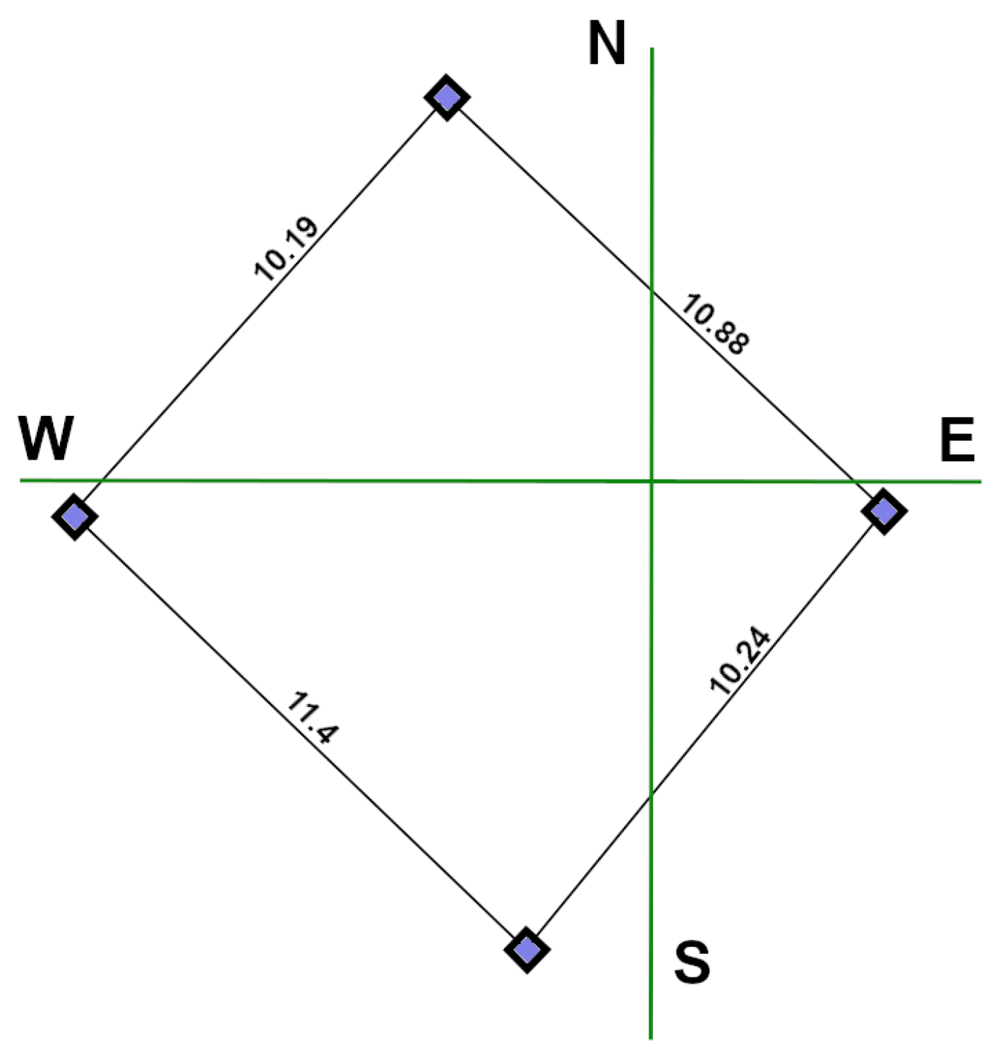
The aperture of the horizontal array is its main characteristic, with the help of which all the main parameters of the array can be calculated. Suppose the array consists of N detectors located at points . In the case of the TEL array, we have four detectors arranged as shown in Figure 1.
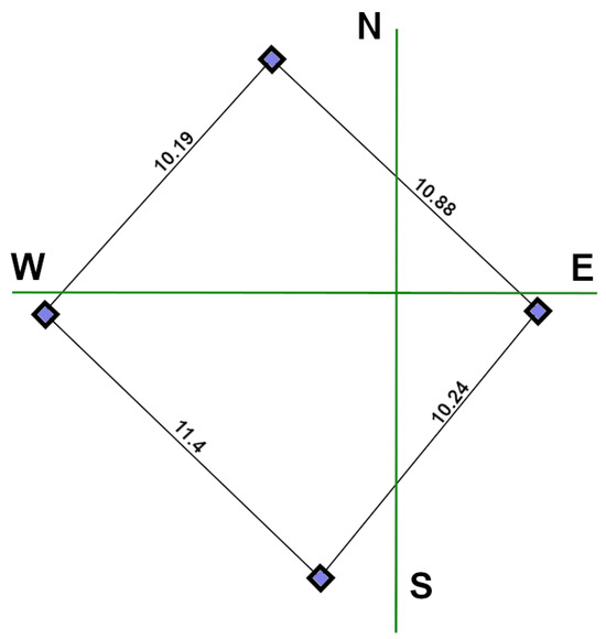
Figure 1.
Layout of the TEL detectors in the attic of the building of Telavi University. Distances shown are in metres.
The aperture of the array as a function of the shower energy E is determined through the following integral:
The characteristic function of the sensitivity region of the installation is
where
X is the vertical air column above the array; are coordinates of all detectors of the array; and are sensitivity thresholds of each detector; E is the energy of primary particle that initiated the shower; R is the distance from the origin of coordinates to the shower axis position (point of intersection of the shower axis with the horizontal plane of the array coordinate system); is the azimuth of this axis position point in the array plane; is the zenith angle of the direction of arrival of the shower; and is the azimuth of the direction of arrival of the shower.
The expected number of shower particles at the position of the i-th detector is given by , and is the distance from the i-th detector to the EAS axis trajectory. Its calculation is obvious.
The calculated number of particles in Equation (2) is determined, firstly, by the Nishimura–Kamata–Greisen formula [5,6] in which the number of particles and the age are determined from the mean cascade curve of a shower with a given energy, and the characteristic transverse radius according to Moliére for a given air density at the array plane is fixed.
These functions for each detector are included in the definition of the characteristic function (Equation (3)). It is taken into account here that not all particles in the shower front reach the detectors; some of them are absorbed in the substance surrounding the setup—in the so-called “”. The quantity is the total thickness of the absorber located above the setup. In the general case, it depends on the spherical angles of the shower arrival direction. The value of is the thickness of a cascade unit for the filtering substance, and the function represents the dependence of the thickness of the atmosphere above the matrix on the zenith angle of the direction of arrival of the shower.
The function appears in the classical theory of electromagnetic cascades [7] as a postulated stationary solution in the variable X. It is related to a parameter s, called the age parameter of the cascade, which defines the postulated stationary solution in the energy variable of the form . The function takes into account the functional forms of the cross sections for pair production and bremsstrahlung in a rather complex way, but practically, it can be assumed that with a good approximation, it is , while .
The characteristic function in Equation (3) actually limits the integration region over R for each set of angles—that is, it sets the maximum allowable distance from the origin to the shower axis.
Let be the limiting distance to the point where the shower axis hits the array plane, which is located in the direction of azimuth . At this distance, the function of the average number of particles (Equation (4)) in each sensor reaches the corresponding limit of the threshold sensitivity . This distance should be found numerically as the point of a jump in the value of the characteristic function in Equation (2) from 1 to 0. In this process, the function is uniquely defined. Using this function, we obtain a simplified expression for aperture (Equation (1)):
Thus, integration over distances to the shower axis has already been carried out. Further integration in the expression (Equation (5)) is complex and cumbersome, and essentially uninteresting. Equation (5) is used for the numerical determination of the aperture of any array for any given shower energy. Further, this function is considered known for a given sensitivity threshold .
2.2. Shower Counting Rate
After the dependence of the aperture on the shower energy, E is calculated with a known vertical atmospheric thickness X above it, a given detector arrangement , and their sensitivity thresholds ; the shower counting rate by this array can then be determined.
Let be the known density of the flux of particles with energy E that initiate the shower in the Earth’s atmosphere.
Here, is the total flux of showers with energy above , and the probability density function of shower energies in the total shower flux (normalised to unity ).
Then, the average frequency of shower registration () by an array with a known aperture is determined (roughly and conditionally) by the integral of the product of the shower flux by the aperture (the minimum energy is a spectrum parameter that does not depend on the properties of the setup; in fact, it is the aperture function that limits the integration limit from below by the threshold energy of the setup):
2.3. Determination of the Average Effective Threshold of Sensitivity of Detectors and the Energy Threshold of the Installation
Let us calculate, in accordance with Equation (7), the possible average frequencies of EAS registration by this array for an arbitrarily specified set of possible sensitivity thresholds of all detectors:
We construct the interpolation polynomial on the basis of m points and obtain an estimate of the real average effective sensitivity of all detectors as a value of P, at the point , which is the experimentally measured counting rate of the array.
3. Luminosity of the TEL Array
The TEL array is shown in Figure 1. Four scintillation detectors with an area of 0.25 were arranged in an almost square geometry at a distance of about 10 m from each other. Vertical thickness of air above the device (X) was 936.35 g/ (820 m altitude) and air density at the location was 1.129 × g/. The width of the coincidence gate was set to 1200 ns. The array trigger required all four detectors to be hit within this time. Each individual detector counting rate was set at 100 Hz, which, given such a coincidence time gate width, resulted in a virtually negligible number of unwanted quadruple coincidence noise registrations.
The presence of a concrete ceiling was also roughly taken into account. It was rather arbitrarily assumed that = 27.5 g . Since the TEL detectors were also surrounded by the walls of the building, to simplify calculations, it was assumed that the “” would surround the protractor uniformly—something like a dome over the installation: it was assumed that absorption in the “” did not depend on the direction of the shower’s arrival.
Using these data, the counting rates of the TEL array were calculated for some arbitrary (but reasonable) possible sensitivity thresholds of all detectors. The energy spectrum of the cosmic ray particles that initiated the extensive air showers was used as reviewed by [8].
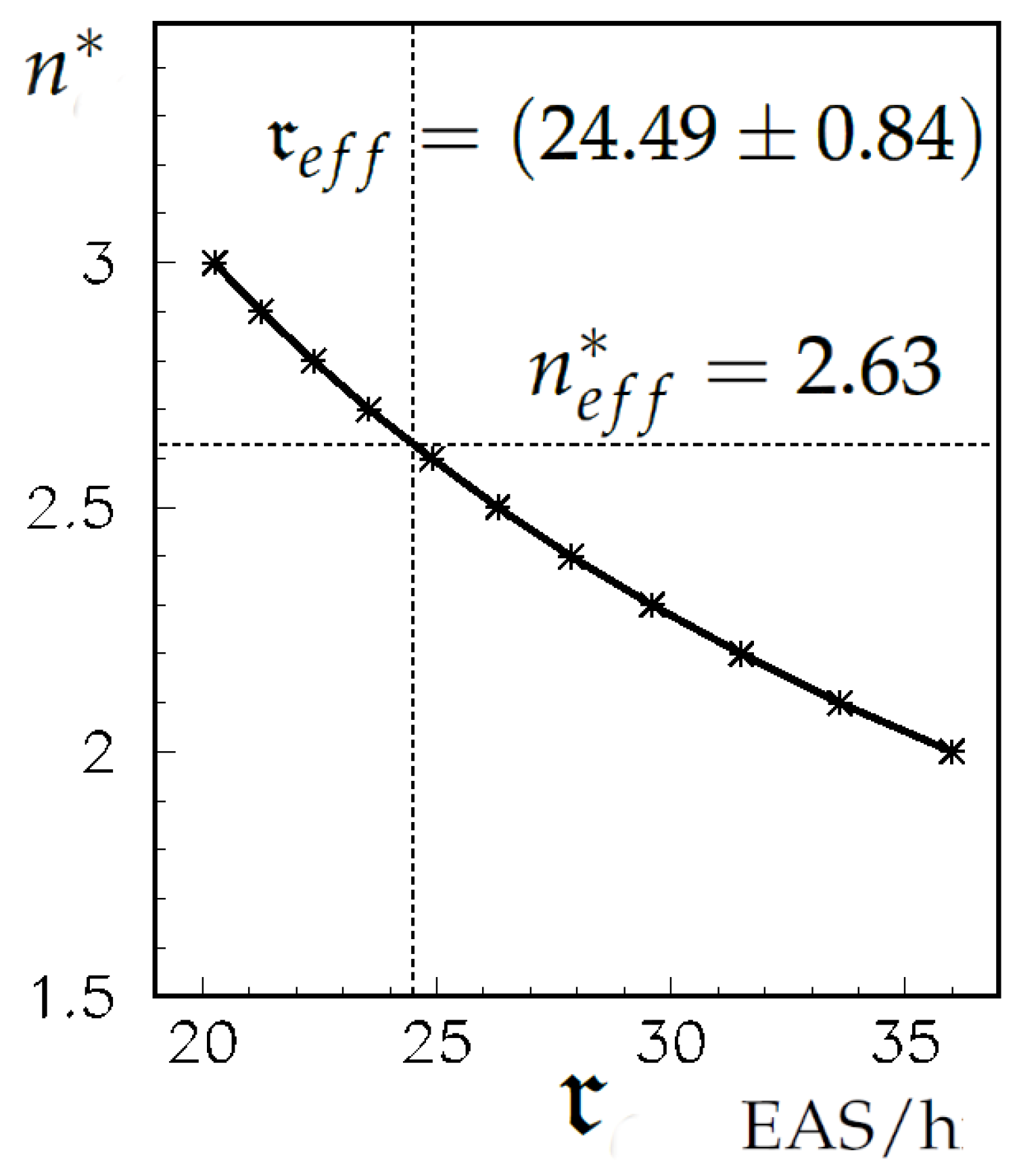
Based on these values, an interpolation polynomial was constructed, which is shown in Figure 2, together with the base points.
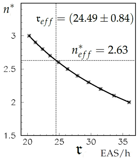
Figure 2.
Each detector threshold as a function of the counting rate of the TEL array.
The counting rate of the TEL array was measured:
Numerically inverting the polynomial P,
we found (see Figure 2) an estimate of the effective sensitivity threshold of the TEL array detectors:
3.1. Ambiguity of the Solution Found
The effective registration threshold of the TEL array detectors has been determined analytically, assuming that it is the same for all detectors. We cannot guarantee this, but the value of more than 2 minimum ionising particle (m.i.p.) is itself questionable. A reasonable discrimination level is 1 m.i.p., and any other setting should have some justification.
This problem is, however, only illusory. In the calculations, the trigger level appears as one of three factors defining the (expected) threshold number of particles at which the Heaviside function changes from 0 to 1, and this, of course, depends on the detector area s and its efficiency , which is understood as the probability of registering a particle crossing the detector surface:
where is the expected density of EAS particles at given point . This quantity is equal to the previously determined . Thus,
and therefore, the actual threshold for particle registration by TEL array detectors can be set at 1 m.i.p., as long as the registration efficiency is correspondingly less than 100%.
3.2. Testing the Effectiveness of TEL Detectors
To address the question of the registration threshold, a method has been proposed to quickly find the efficiency of detectors using real minimally ionising particles—incoherent cosmic ray muons. These reach the Earth’s surface at frequencies of hundreds per per second. At the same time, as the name suggests, they arrive independently, so that with the coincidence gate open for a few hundred nanoseconds, there are virtually no cases of more than one particle passing through the surface of a detector such as the TEL array while the gate is open.
We placed the four TEL array detectors on top of each other in the geometry of the telescope. If they all have 100% efficiency, an incoming incoherent muon would mostly produce a signal in all the detectors (1234). In rare cases, if it is close to the edge, it could hit the bottom three (-234) or the top three detectors (123-), and even more rarely, the top two (12- -), the bottom two (- -34), and very exceptionally, if it is a practically horizontal muon, it could hit the pair of detectors in the middle of the telescope (-23-).
If the efficiency of the detectors is not 100%, events will occur when, for example, the top detector is hit, the second detector does not give a large enough signal, and the two lower detectors register the passage of a particle (1-34), etc. The total number of possible coincidences (double, triple, and quadruple) is 11. By measuring the frequency of occurrence of each of these events, the efficiency of all four TEL array detectors can be determined. The coincidence time gate width for the system of detectors aligned with the telescope geometry was reduced to 250 ns to also eliminate unwanted random double and triple coincidences.
If it is assumed that the detectors have efficiencies that are not 100%, then the simple geometry of the tracks must be supplemented by the respective probability Bernoulli trials to determine whether the detector through which the particle will pass will give a sufficiently strong signal. These quantities define the detector efficiencies .
The whole algorithm of searching for the most likely values of efficiency is, in fact, a simple geometric puzzle. First, it counts the muons that passes through all the detectors (top and bottom are enough). Of course, for each trajectory, the respective solid angle is calculated, and the flux corrected by is multiplied by the respective efficiency factors. For pattern ‘1234’, it is ; for ‘-234’, it is ; for ‘-23-’, it is ; and so on. A similar procedure should be used for particles that hit detectors 2, 3, and 4 and that do not hit detector 1. The corresponding is also added to the variable ‘-234’, etc. Such a similar procedure should be applied for muons hitting 1, 2, and 3 (but not 4) and in cases of hitting detectors 2 and 3 but not detectors 1 nor 4. Finally, the contributions of the muons hitting detectors 3 and 4 (but not 1 nor 2) are totalled.
After performing all the geometric integrations and normalising the sum of counts in each configuration to the number of cases measured experimentally, we determine the value of the statistic. Minimising this quantity in the four-dimensional cube of efficiencies leads to finding the best matching efficiencies of all four detectors.
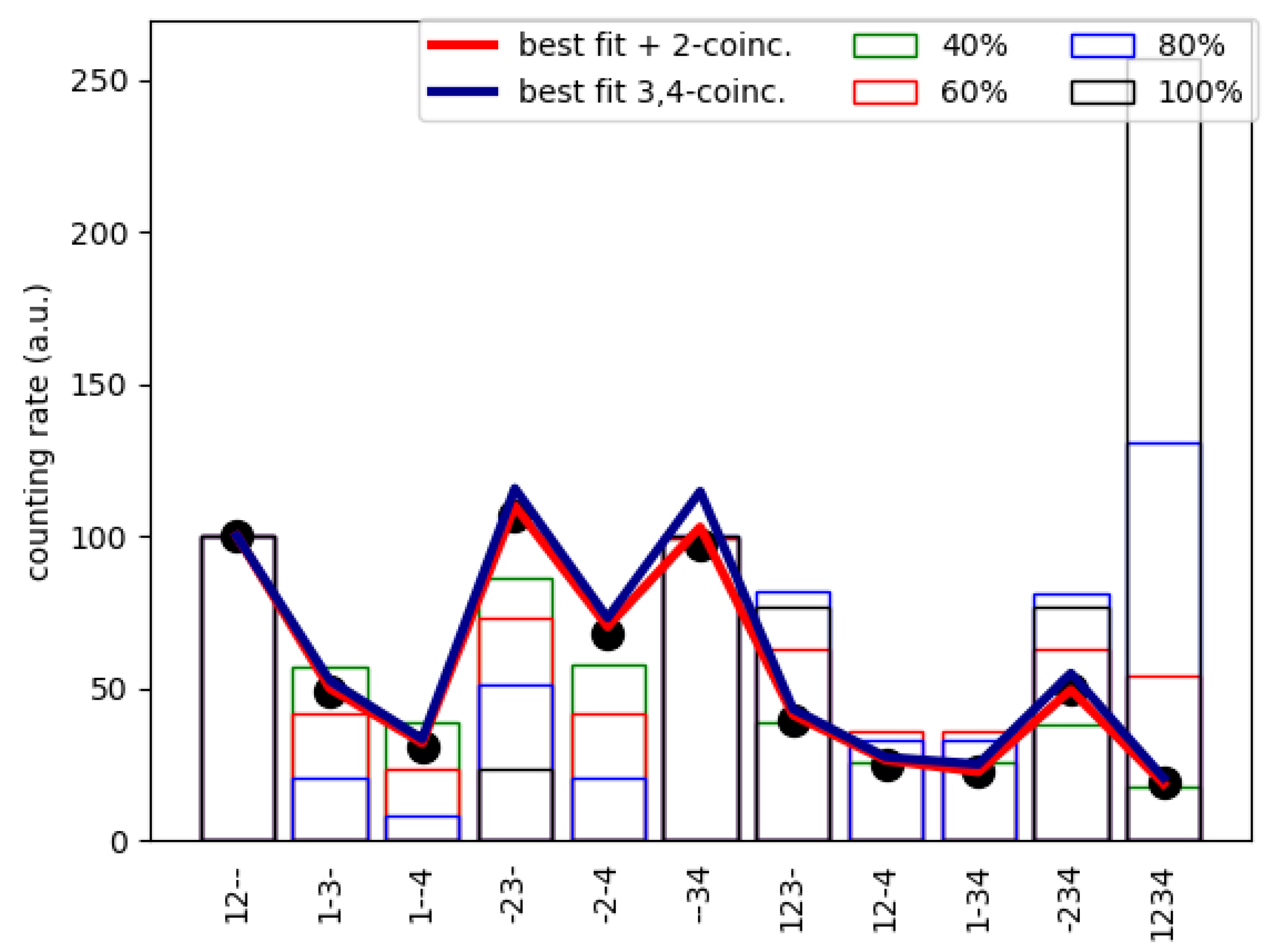
The results are shown in Figure 3. As can be even seen from the last bar of the histogram, the efficiency of the TEL detectors is far from 100%. If we take for the fitting procedure only the cases of 3-fold and 4-fold coincidence, which we are certain do not contain any random registrations but only actual cases of the charged particle passing through the telescope, then the best-fit detector efficiencies are 35%, 45%, 41%, and 40% for detectors 1, 2, 3, and 4, respectively. When we performed the fitting including all 11 combinations shown in Figure 3, the best-fit values changed slightly to 35%, 45%, 43%, and 42%, which is not a significant change, but shows the correctness of the telescope and the fit method, while assuring us that the double coincidences also do not contain noise registration, which we have ensured by reducing the width of the time gate as mentioned above. We can therefore say that the efficiency of TEL detectors is in the order of 40%.
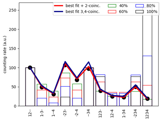
Figure 3.
Fitting the TEL detector efficiencies to the measured recording rates of the different possible coincidences. The measurements are shown as black circles and are normalised to 100 for ‘12- -’ coincidence. The coloured histograms show, for illustration, the predictions for a few different efficiencies (the same for all detectors). The black broken line shows the fit considering only triple and quadruple coincidence (last 5 points), while the red broken line is the fit for all 11 points (see text for details).
The analytically found value of = 2.63, obtained by assuming , converts to at , practically 1 m.i.p. This result proves, firstly, the correctness of the analytical estimates and the correctness of the operation of the TEL array, and, secondly, the validity of the proposed method for determining the detector efficiency.
4. Distribution of Cosmic Ray Particle Energies Available for Observations by the TEL Array
The actual role of the luminosity function of a particular array is reduced to an energy-dependent reduction of the flux in the energy spectrum of all showers () to the flux of only those showers that the given array is capable of recording. Consequently, the observed energy distribution is proportional to the product:
Figure 4 shows the distribution of shower energies accessible for observations by the TEL array obtained with Equation (14) as a dashed line. The spectrum drops very quickly for energies below TeV.
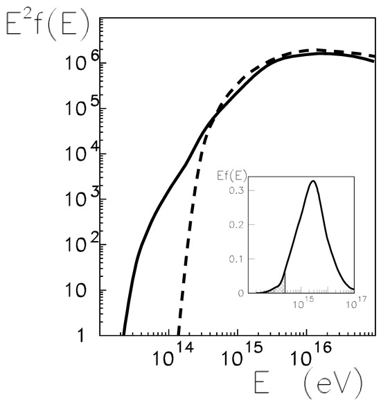
Figure 4.
Spectrum of primary particle energy for showers observed by the TEL array calculated by the analytical method (dashed line) and simulation calculations (black dots and solid line). The inset figure shows the spectrum on a log-log scale, rescaled so that the area under the curve corresponds to the particle flux in the given energy interval. The shaded area indicates the difference between the spectrum obtained from the simulation and the analytical solution.
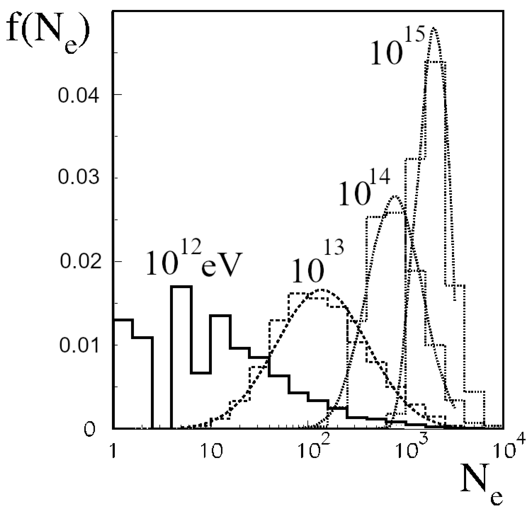
As shown above, analytical considerations make several assumptions that are undoubtedly approximations of physical reality. One of the most important is the lack of consideration of fluctuations in the development of showers. These are essentially of three types. The first and most important are fluctuations in the size of the shower, here still understood as the number of charged particles (mainly electrons and positrons) at the observation level, which must naturally occur even for a fixed energy and type of primary particle. Figure 5 [9] shows how the number of particles varies for proton showers with fixed energies from 1 TeV to 1 PeV. It is worth noting that the higher the energy, the relatively narrower the distributions are, and therefore, the fluctuations in the size of the shower are relatively less significant. The second type of fluctuation is also associated with the variability in the evolution of the shower. Even with the same fixed primary energy and the same size of the shower, the transverse distributions of the particles in the shower can be different. Finally, the third type are fluctuations in the density of particles in a shower, or more precisely, fluctuations in the number of particles that fall into a detector of a given size at a given location. In a first approximation, they are Poissonian, although a closer examination of the subject shows [9] that we can expect deviations from the simple assumption of independence of the particles in the shower.

Figure 5.
Particle number fluctuations in showers initiated by primary vertical protons of different energies. The curves showing the shapes of the distributions for the three highest energies are fits of the LogNormal distributions.
All these effects can be seen in the results of programmes that simulate the evolution of the shower.
5. Simulation Results
The simulated extensive air showers used here were obtained with the CORSIKA programme [10] developed over 30 years ago in Karlsruhe for the KASCADE experiment [11,12]. CORSIKA has been significantly extended and developed since then. Over time, new functions have been added and computational capabilities have been increased to meet the simulation needs of new cosmic ray experiments, and it is still used for simulations even at the highest observed energies (even up to eV).
The already linked programme requires the current simulation parameters to be set. For typical shower simulations, the default set of simulation parameters already built into the programme is selected. However, if the CORSIKA is being used for a more unusual purpose, such as, for example, detailed simulations of a small shower array, then the values of some parameters need to be set particularly carefully. For the purposes of this work, we used CORSIKA to simulate the TEL array trigger. We had to count detector hits by single particles, so we could not use any thinning options. We set the minimum energy of the tracked particles to 3 MeV.
Regarding the high-energy interaction model, in this work, we analysed the simulation results of the CORSIKA programme (version 7.7401) with the setup of the EPOS LHC strong interaction model [13] (v3400). Our interest is focused on particle energies of the ‘knee’, around – eV, which are available to a large extent for some time in accelerator experiments. All high-energy interaction models implemented in CORSIKA were initially fitted to the accelerator results and all gave very similar results in this energy region. Discrepancies could only appear when these models were extrapolated to the highest energies.
The low-energy interaction model CORSIKA is equipped with three options: GHEISHA [14], FLUKA (FLUktuierende KAskade) [15], and UrQMD (Ultrarelativistic Quantum Molecular Dynamics) model [16]. For the purposes of this work, we can expect that the interaction model chosen below GeV is not critical. We used GHEISHA here.
The well-known electromagnetic processes are responsible for the general properties in the relatively small showers. These are described in CORSIKA by the EGS4 (Electron Gamma Shower) package [17].
For the present work, we performed simulations for primary protons with energies from to eV.
Charged particles reaching observation levels in the simulated shower were randomly sampled by an array of TEL detectors located up to 100 m from the axis of the shower, and it was checked in each case whether all four of them would be hit by the shower particles, assuming a detector efficiency of 40%.
The resulting ratio is proportional to the probability that the shower was recorded by a TEL array, and then it is convolved with the primary particle spectrum . The resulting energy spectrum of the showers recorded by the TEL array is shown in Figure 4 as a smooth black solid curve moving through them.
As can be seen, starting from energies of eV, the simulation results are in good agreement with the results of the analytical calculations. The small systematic discrepancy is due to the fact that the mean transverse distributions and the dependence of the mean shower size on the energy (and on the angles of incidence) assumed in the calculations are not in absolute agreement with the results of the simulations (with the assumed interaction models). The search for absolute agreement is already not justified because of the discrepancies in the modelling of showers in CORSIKA.
On the other hand, below eV, the truncation occurs much faster in the analytical method than in the simulations. This is an obvious effect of not taking fluctuations into account, as mentioned above. In Figure 4, this effect is clearly visible, especially in the inset figure with a smaller line-logarithmic scale, where the area under the curve corresponds to the flux of primary cosmic rays in a given range of particle energies. This effect is clearly important for the estimate of the rate with which the station detects showers, but the significance is not large. The dashed area in Figure 4 represents about 4% of the total area under the energy spectrum curve. A more important finding seems to be the fact that the lower energy threshold recorded by the small array is shifted. The actual truncation in the simulation calculations is about an order of magnitude lower than that would be obtained from analytical calculations averaging everything. Estimating and attempting to determine the number of times that small instruments register cosmic ray showers initiated by particles around (and below) 100 TeV is not in itself a task of fundamental or even great cognitive importance. Nevertheless, the mere awareness, not to mention the quantitative knowledge, that one can register the remains of showers initiated by particles with energies below 100 TeV, can be of importance in fields far from the mainstream of cosmic ray research, where cosmic rays are an unwanted and undesirable side effect. Examples include biological studies in low-background laboratories.
6. Summary
We have shown that the energy spectrum of primary cosmic ray particles recorded by a small shower array, such as the GELATICA network station at Telavi Iakob Gogebashvili State University (TEL), obtained by an analytical approach is consistent with accurate simulation calculations based on sophisticated programmes like CORSIKA.
The analytical approach assumes that for a given primary particle energy, its mass and angle of arrival, the size of the shower recorded at a given depth, and the lateral distribution of the charged particles in the shower are always identical to the theoretically justified expected values and distributions. It is also assumed that the detectors sense the average density at a given point and generate a trigger signal when a certain value, considered as the registration threshold, is exceeded.
At first sight, these assumptions seem rather crude, but the shown agreement with the CORSIKA simulation results proves that they are sufficiently accurate (with a systematic bias of about a few per cent).
The detector registration threshold in the analytical method is determined from the measured EAS registration rate, but the value obtained this way is not completely unique. It does not necessarily correspond to the detector amplitude signal level. The threshold needs to be combined with the detector efficiency. We have proposed a method to measure the absolute efficiency of the detectors.
By applying this method to the TEL array detectors, their efficiency was determined to be of about 40%, which, combined with the analytically determined recording rate, gave an actual threshold detector amplitude of 1 m.i.p.
The analytically determined aperture of the TEL array unambiguously gives the energy distribution of the primary cosmic ray particles that trigger the large atmospheric showers recorded by the instrument. The spectrum obtained in this way has a very abrupt cut-off at low energies (estimated at ∼200 TeV). Such an abrupt cut-off is caused by the fact that the assumptions of the analytical method do not take into account any fluctuations. Any fuzziness in the parameters of the actual shower leads to a smearing and smoothing of any sudden changes in the spectrum.
Simulation methods inherently account for most of the random deviations from the various mean parameters of extensive air showers. A much smoother truncation and a lower threshold for EAS registration up to 20 TeV are clearly evident from the CORSIKA results shown. However, it is worth noting that the EAS registration rate of the TEL apparatus is hardly affected by the differences in the determination of the lower energy threshold.
In the context of the search for cosmic ray ensembles, it must be stated that the reliable identification of such events requires knowledge of the detection capabilities of the (global) network of detection stations, and in particular, the minimum energy at which showers can be effectively recorded. The accurate modelling of the TEL station response and the comparison of analytical estimates with CORSIKA simulations provided a quantitative basis for defining the energy range available to a GELATICA station network. This is particularly important for the distinction between random background recordings and real, physically correlated registrations of extensive air showers in a cosmic ray ensemble. By correctly defining the lower energy threshold, it will be possible to filter out background events and improve the selection criterion for potential cosmic ray ensembles. This will increase the importance of their potential detection and the astrophysical significance of such detections. Furthermore, a thorough understanding of the shower registration limit of the analysed TEL-type station allows us to optimise the search for distant coincidences in the whole network of all GELATICA stations. By setting a common threshold for the energy of the recorded showers for all stations, we improve the reliability of potential observations of long-range correlations between stations. This is crucial for the search for large-scale structures in the highest-energy-particle flux in cosmic rays or rare ensemble events.
Finally, it should be noted that there are many publications that obviously used simulation methods to determine the parameters of the cosmic ray surface array. With the increase in computing power in recent years, this has become a common tool and has been used so often that other methods have almost been forgotten. Practically all current publications on these topics operate on the results of CORSIKA-type programmes, without delving into the physics and treating the simulation results as a matter that is obvious and undeniably true. The discrepancies in interpretation resulting from the different interaction models and the simplifications used are not surprising. They do not cause physical confusion. In the 20th century, analytical and semi-analytical solutions performed similar tasks. However, as a result of the above exchange of analysis methods, there has been little recent work comparing the two. A significant comparative publication, if one has been produced lately, is not widely known. Thus, this work provides some additional, perhaps not entirely physical, value.
Author Contributions
Conceptualisation, T.W. and M.S.; Data curation, R.B., A.I., V.K. and I.I.; Formal analysis, T.W.; Funding acquisition, M.S.; Investigation, R.B., A.I., V.K. and I.I.; Methodology, T.W. and M.S.; Project administration, M.S.; Resources, R.B., A.I., V.K. and I.I.; Supervision, T.W. and M.S.; Validation, R.B., A.I. and I.I.; Writing—original draft, T.W.; Writing—review and editing, M.S. and R.B. All authors have read and agreed to the published version of the manuscript.
Funding
This work was supported by the Shota Rustaveli National Science Foundation of Georgia (SRNSFG) FR 23-1964.
Data Availability Statement
The original data presented in the study are available on request from the corresponding author.
Acknowledgments
The authors are grateful to other members of the GELATICA team for their technical support.
Conflicts of Interest
The authors declare no conflicts of interest.
References
- GEorgian Large-Area Angle and TIme Coincidence Array. Available online: https://gelatica.tsu.ge/ (accessed on 30 January 2025).
- Verbetsky, Y.; Svanidze, M.; Ruimi, O.; Wibig, T.; Kakabadze, L.; Homola, P.; Alvarez-Castillo, D.E.; Beznosko, D.; Sarkisyan-Grinbaum, E.K.; Bar, O.; et al. First Results on the Revealing of Cognate Ancestors among the Particles of the Primary Cosmic Rays That Gave Rise to Extensive Air Showers Observed by the GELATICA Network. Symmetry 2022, 14, 1749. [Google Scholar] [CrossRef]
- Homola, P.; Beznosko, D.; Bhatta, G.; Bibrzycki, Ł.; Borczyńska, M.; Bratek, Ł.; Budnev, N.; Burakowski, D.; Alvarez-Castillo, D.E.; Almeida Cheminant, K.; et al. Cosmic-Ray Extremely Distributed Observatory. Symmetry 2020, 12, 1835. [Google Scholar] [CrossRef]
- Dhital, N.; Homola, P.; Alvarez-Castillo, D.; Góra, D.; Wilczyński, H.; Almeida Cheminant, K.; Poncyljusz, B.; Mędrala, J.; Opiła, G.; Bhatt, A.; et al. Cosmic ray ensembles as signatures of ultra-high energy photons interacting with the solar magnetic field. J. Cosmol. Astropart. Phys. 2022, 2022, 038. [Google Scholar] [CrossRef]
- Wilson, J.G.; Greisen, K. Progress in Cosmic Ray Physics; North-Holland: Amsterdam, The Netherlands, 1956; Volume 3. [Google Scholar]
- Kamata, K.; Nishimura, J. The Lateral and the Angular Structure Functions of Electron Showers. Prog. Theor. Phys. Suppl. 1958, 6, 93–155. [Google Scholar] [CrossRef]
- Rossi, B. Cosmic Rays; McGraw–Hill, Inc.: London, UK, 1966. [Google Scholar]
- Navas, S.; Amsler, C.; Gutsche, T.; Hanhart, C.; Hernández-Rey, J.J.; Lourenço, C.; Masoni, A.; Mikhasenko, M.; Mitchell, R.E.; Patrignani, C.; et al. Review of particle physics. Phys. Rev. D 2024, 110, 030001. [Google Scholar] [CrossRef]
- Wibig, T. Intermittent behaviour in small CORSIKA showers. J. High Energy Astrophys. 2023, 40, 11–18. [Google Scholar] [CrossRef]
- Heck, D.; Knapp, J.; Capdevielle, J.N.; Schatz, G.; Thouw, T. CORSIKA: A Monte Carlo Code to Simulate Extensive Air Showers; KZKA-6019; Forschungszentrum Karlsruhe GmbH: Karlsruhe, Germany, 1998. [Google Scholar]
- Antoni, E.T.; Apel, W.D.; Badea, F.; Bekk, K.; Bercuci, A.; Blümer, H.; Bozdog, H.; Brancus, I.M.; Büttner, C.; Chilingarian, A.; et al. The cosmic-ray experiment KASCADE. Nucl. Instrum. Methods Phys. Res. Sect. A Accel. Spectrometers Detect. Assoc. Equip. 2003, 513, 490–510. [Google Scholar] [CrossRef]
- Klages, H.O.; KASCADE Collaboration; Apel, W.D.; Bekk, K.; Bollmann, E.; Bozdog, H.; Brâncuş, I.M.; Brendle, M.; Chilingarian, A.; Daumiller, K.; et al. The Extensive Air Shower Experiment Kascade—First Results. In Proceedings of the 25th International Cosmic Ray Conference (ICRC1997), Durban, South Africa, 28 July–8 August 1998; Volume 8, pp. 297–306. [Google Scholar] [CrossRef]
- Pierog, T.; Karpenko, I.; Katzy, J.M.; Yatsenko, E.; Werner, K. EPOS LHC: Test of collective hadronization with data measured at the CERN Large Hadron Collider. Phys. Rev. C 2015, 92, 034906. [Google Scholar] [CrossRef]
- Fesefeldt, H. The Simulation of Hadronic Showers -Physics and Applications-; Physikalisches Institut RWTH Aachen, FRG, 1985. Available online: http://cds.cern.ch/record/162911/files/CM-P00055931.pdf (accessed on 30 January 2025).
- Mazziotta, M.; Cerutti, F.; Ferrari, A.; Gaggero, D.; Loparco, F.; Sala, P. Production of secondary particles and nuclei in cosmic rays collisions with the interstellar gas using the FLUKA code. Astropart. Phys. 2016, 81, 21–38. [Google Scholar] [CrossRef]
- Bleicher, M.; Zabrodin, E.; Spieles, C.; Bass, S.A.; Ernst, C.; Soff, S.; Bravina, L.; Belkacem, M.; Weber, H.; Stöcker, H.; et al. Relativistic hadron-hadron collisions in the ultra-relativistic quantum molecular dynamics model. J. Phys. G Nucl. Part. Phys. 1999, 25, 1859. [Google Scholar] [CrossRef]
- Nelson, W.R.; Hirayama, H.; Rogers, D.W. Electron-photon transport using the EGS4 (Electron Gamma Shower) Monte Carlo Code. In Proceedings of the Transactions of the American Nuclear Society: 1986 Annual Meeting, Reno, NV, USA, 15–19 June 1986; Volume 52. [Google Scholar]

Disclaimer/Publisher’s Note: The statements, opinions and data contained in all publications are solely those of the individual author(s) and contributor(s) and not of MDPI and/or the editor(s). MDPI and/or the editor(s) disclaim responsibility for any injury to people or property resulting from any ideas, methods, instructions or products referred to in the content. |
© 2025 by the authors. Licensee MDPI, Basel, Switzerland. This article is an open access article distributed under the terms and conditions of the Creative Commons Attribution (CC BY) license (https://creativecommons.org/licenses/by/4.0/).