Triple-Flow Dynamic Graph Convolutional Network for Wind Power Forecasting

Abstract

Wind energy is a clean but intermittent and volatile energy source, and its large-scale integration into power systems poses great challenges to ensuring safe and stable operation and achieving scheduling optimization and effective energy planning of the power systems. Accurate wind power forecasting is an effective way to mitigate the impact of wind power instability on power systems. However, wind power data are often in the form of multivariate time series. Existing wind power forecasting research often directly models the temporal and spatial characteristics of coupled wind power time-series data, ignoring the heterogeneity of time and space, thereby limiting the model’s expressive power. To address the above problems, we propose a triple-flow dynamic graph convolutional network (TFDGCN) for short-term wind power forecasting. The proposed TFDGCN is a symmetric dynamic graph neural network with three branches. It decouples and learns features of three different dimensions: within a wind power variable sequence, between sequences, and between wind turbines. The proposed TFDGCN constructs dynamic sparse graphs based on cosine similarities within variable sequences, between variable sequences, and between wind turbine nodes, and feeds them into their respective dynamic graph convolution modules. Afterwards, TFDGCN utilizes linear attention encoders which fuse local position encoding (LePE) and rotational position encoding (RoPE) to learn global dependencies within variable sequences, between sequences, and between wind turbines, and provide prediction results. Extensive experimental results on two real-world datasets demonstrate that the proposed TFDGCN outperforms other state-of-the-art methods. On the SDWPF and SD23 datasets, the proposed TFDGCN achieved mean absolute error values of 37.16 and 14.63, respectively, as well as root mean square error values of 44.84 and 17.56, respectively.

1. Introduction

Wind energy has received widespread attention due to its renewable, environmentally friendly, and sustainable characteristics. However, as a clean energy source with significant intermittent and fluctuating characteristics, its large-scale grid connection poses many great challenges, including the safe and stable operation of the power system, dispatch optimization, and energy planning [1]. Accurate wind power forecasting (WPF) can be used to guide power dispatching and grid deployment [2,3], and therefore it is an effective way to mitigate the impact of wind power instability on power systems [4].

In recent years, deep learning has been widely used in wind power forecasting tasks due to its powerful nonlinear fitting and complex data modeling capabilities. Liu et al. [5] proposed a short-term wind power forecasting framework based on wavelet transform (WT) denoising and multi-feature long short-term memory (LSTM) networks. Li et al. [6] decomposed wind power sequences using VMD, and grouped these sequences by complexity, and they then implemented forecasting using a dual-channel network composed of an informer and a temporal convolutional network (TCN) informer. Wang et al. [7] divided wind farm clusters based on empirical orthogonal functions and combined multi-level quantiles with WaveNet with multi-head self-attention to achieve ultra-short-term interval power multi-step prediction. Zhu et al. [8] proposed a wind speed prediction method that combines a non-stationary Transformer with dynamic data distillation and wake effect correction. Although the above methods have achieved some degree of success in capturing temporal dependencies of wind power data, wind power prediction is by no means a simple time series prediction problem. The power generation of a wind turbine is determined by its own historical pattern and the conditions of related wind turbines [9]. Therefore, the wind power prediction task is essentially a spatiotemporal prediction problem that requires simultaneous characterization of temporal laws and spatial characteristics.

Due to the advantages of graph neural networks (GNNs) in modeling spatial dependencies, many studies have used GNNs to capture dependencies between wind turbines [10]. These methods use GRU or CNN and their related variants to capture temporal features, which are combined with spatial features captured by GNNs to form spatiotemporal joint features. For example, Daenens et al. [11] constructed a graph structure based on line-of-sight visibility and used generalized graph convolution (GENConv) and LSTM to extract spatiotemporal dependencies to achieve offshore wind farm power prediction. An et al. [12] used electrical connection relationships to construct a graph structure and embedded diffusion graph convolution (Diffusion Graph Convolution) into a gated recurrent unit (GRU) to capture spatiotemporal dependencies to achieve ultra-short-term power prediction. Yang et al. [13] divided wind farm clusters through deep attention embedded graph clustering (DEAGC) and used TimesNet to capture multi-cycle time features after data correction and screening. Zhao et al. [14] constructed a multi-graph structure and integrated TCN with spatiotemporal attention mechanism to achieve ultra-short-term wind power interpretable prediction. Zhao et al. [15] modelled wind farms as nodes, calculated edge weights based on distance and Pearson correlation coefficient, and constructed a static adjacency matrix. They used two spatiotemporal graph convolutional layers (STGCN) and an output layer to achieve the effect of ultra-short-term wind power prediction. All the aforementioned methods constructed static graphs using wind turbines as nodes and information such as their correlation and geographic distance as edges. However, the actual spatial connections between wind turbines are determined not only by their location but also by time-varying meteorological conditions such as wind speed, direction, and humidity. Static graphs with fixed structure and edge weights may not capture these dynamic changes well.

Since it is difficult to use static graphs to capture spatial-temporal correlations, researchers have begun to explore the application of dynamic graph models in wind power prediction. For example, in [9], the authors integrated geographic distance graphs, semantic distance graphs, and learnable parameter matrices, and they dynamically optimized the graph structure through a spatial attention mechanism, and then captured spatiotemporal dependencies by combining an Attentional Graph Convolutional Recurrent Network (AGCRN) with LSTM. Yang et al. [10] proposed a method for ultra-short-term wind power prediction for large-scale wind farm clusters based on dynamic spatiotemporal graph convolution. This method abstracts the wind farm into a graph and dynamically adjusts it. It combines spatial graph convolution with temporal graph convolution to model temporal and spatial dependencies and introduces multi-task learning (MTL) to simultaneously output multi-step prediction results for multiple wind farms. Han et al. [16] used dynamic graph convolution to capture the dynamic spatial correlation of wind farm clusters and used BiLSTM and Transformer to mine the bidirectional temporal dependencies of wind power, thus achieving power prediction for wind farm clusters. Song et al. [17] proposed a wind power forecasting method based on dynamic graph convolution and multi-resolution CNN. This method uses multi-resolution CNN and dynamic graph convolution to extract temporal and spatial features, respectively. Dong et al. [18] extracted the temporal and spatial features of wind power data through directed graph convolution and TCN, respectively, and they realized the power forecasting of wind farm clusters. Although dynamic graphs can dynamically capture spatial features, recent studies on time series modeling have shown that the dependencies between time and space are heterogeneous [19]; time dependencies are usually reflected as dynamic characteristics within the sequence of wind turbine-related variables (such as changes in wind speed, wind direction, or temperature over time), while spatial dependencies are often manifested as cross-sequence relationships between wind turbine variables (such as the correlation between wind speed and wind direction) or spatial dependencies between wind turbines. Existing dynamic graph-based wind power forecasting methods often attempt to extract features simultaneously from the coupled temporal and spatial dimensions. Due to the fundamental differences between these two types of dependencies, jointly modelling them can lead to information entanglement in the dependency representation during feature learning and thus limit the model’s expressive power. Furthermore, existing methods create adjacency graphs with numerous links, and redundant noise in the graph may interfere with the model’s learning of core dependencies, reducing forecasting performance.

To address the above issues, this research proposes a short-term wind power forecasting method based on a triple-flow dynamic graph convolutional network (TFDGCN). Our contributions are as follows:

• We propose a method for constructing dynamic sparse graphs for wind turbines based on cosine similarity. This method dynamically constructs three sparse graphs based on similarities within variable sequences, between variable sequences, and between nodes (wind turbines). This method effectively describes the relationships within wind turbine variable sequences, between sequences, and between wind turbines while reducing computational complexity.
• We propose TFDGCN, which features a symmetric triple-flow architecture. It decouples and learns relationships across three dimensions, namely, within variable sequences, between sequences, and between wind turbines, represented by three sparse dynamic graphs. TFDGCN also uses linear attention to capture global information across the three dimensions.
• We conduct extensive experiments on two real-world wind farm datasets to validate the effectiveness of TFDGCN. TFDGCN outperforms the baseline methods on both wind farm datasets. Furthermore, we demonstrate the effectiveness of various components of TFDGCN through ablation experiments.

The rest of this paper is organized as follows: Section 2 details the problem studied in this research and formally defines the wind power prediction problem. The proposed TFDGCN is presented in Section 3. This is followed by the simulation results reported in Section 4. Finally, Section 5 concludes this paper.

2. Problem Statement

Wind power forecasting for wind farms can reflect three types of correlations: (1) Variable correlation: the various characteristic variables of wind turbines, such as wind speed, wind direction, and temperature, do not act independently. They are interrelated and influence each other, jointly determining wind power. (2) Temporal correlation: continuous wind power data readings form a time series. This means that the data observed at the current moment is correlated with data observed at past moments. This correlation allows for future power forecasts through historical data analysis. (3) Spatial correlation: different wind turbine nodes within the same wind farm may have similar characteristics (e.g., wind speed, wind direction, temperature, power) at the same moment. The correlation between wind turbine nodes with similar characteristics is essentially spatial correlation.

We capture the spatiotemporal correlations of the three types mentioned above through three spatiotemporal dynamic graphs. Namely, we establish dynamic graphs $G_V$ based on variable correlation, $G_T$ based on temporal similarity, and $G_N$ based on spatial correlation. The construction methods of these three dynamic graphs will be detailed in Section 3.1.

Given a multidimensional data set $\chi =\left\{X^1,X^2,\dots ,X^n\right\}\in R^{N\times T\times F}$ observed in a wind farm, $N$ is the number of wind turbines in the wind farm, $T$ is the total time, and $F$ is the measured data of the wind turbines. Where $X^i\in R^{1\times T\times F}$ represents the data observed by the $i$th wind turbine. Our goal is to learn a function f from the historical observation value ${\chi }^{\prime }\in R^{N\times S\times F}$ of the time window of length $S$, and predict the wind power of the future time window of length $S^{\prime }$, as shown below:

$$\left[\begin{array}{cccc}{\widehat{X}}_{(t+1)}^1& {\widehat{X}}_{(t+2)}^1& \dots & {\widehat{X}}_{(t+S^{\prime })}^1\\ {\widehat{X}}_{(t+1)}^2& {\widehat{X}}_{(t+2)}^2& \dots & {\widehat{X}}_{(t+S^{\prime })}^2\\ ⋮& ⋮& \ddots & ⋮\\ {\widehat{X}}_{(t+1)}^N& {\widehat{X}}_{(t+2)}^N& \dots & {\widehat{X}}_{(t+S^{\prime })}^N\end{array}\right]=f\left(\left[\begin{array}{cccc}{X}_{(t-S+1)}^1& X_{(t-S+2)}^1& \dots & X_{(t)}^1\\ X_{(t-S+1)}^2& X_{(t-S+2)}^2& \dots & X_{(t)}^2\\ ⋮& ⋮& \ddots & ⋮\\ X_{(t-S+1)}^N& X_{(t-S+2)}^N& \dots & X_{(t)}^N\end{array}\right],G_V,G_T,G_N\right)$$

(1)

In the above, $\left\{{\widehat{X}}_{(t+1)}^i,{\widehat{X}}_{(t+2)}^i,\dots ,{\widehat{X}}_{(t+S^{\prime })}^i\right\}\in R^{N\times S^{\prime }\times 1}$ is the wind power predicted by the $i$th wind turbine in time window $S^{\prime }$ at time $t$.

3. Methodology

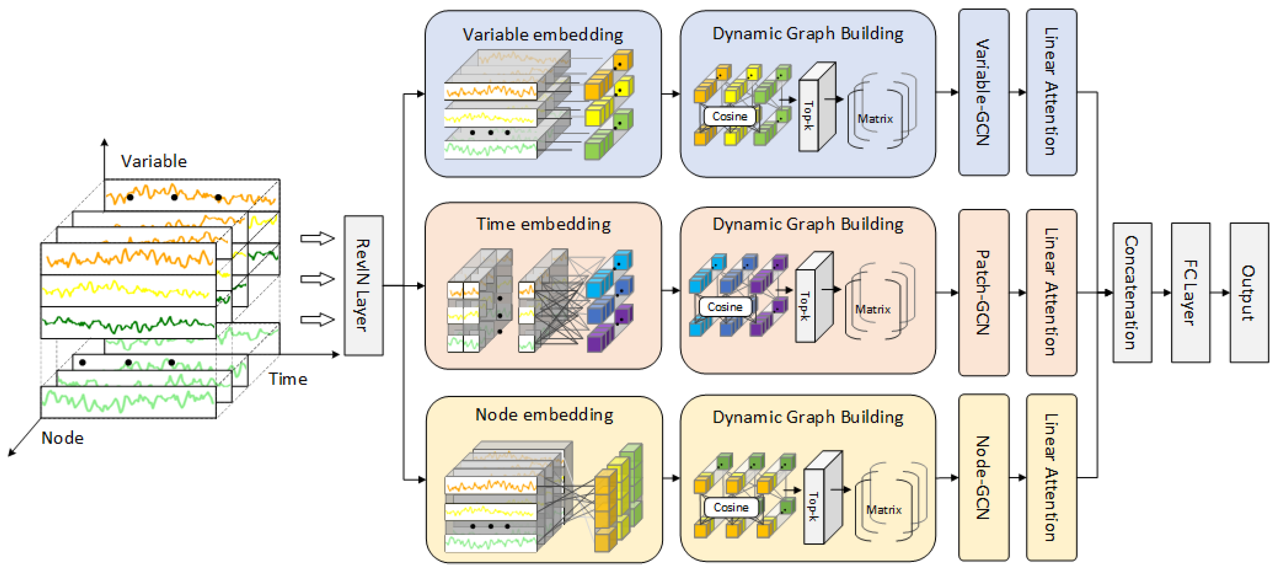
The proposed TFDGCN network architecture is shown in Figure 1. The input data for TFDGCN is multivariate wind power time series data. The coordinate system in Figure 1 can be used to illustrate the variable correlation, temporal correlation, and spatial correlation inherent in these multivariate time series data. In Figure 1, the Variable axis represents wind turbine time series variables such as: wind speed, wind direction, temperature of the surrounding environment, temperature inside the turbine nacelle, nacelle direction, pitch angle of blade, reactive power and active power. The Variable axis describes the relationship between multivariate time series. The Time axis represents the time series, which is the data sequence formed by the changes in wind turbine variables over time. The Time axis reflects the changes in different time slices within a variable’s time series, that is, the change in the variable over time. The Node axis represents the characteristics of wind turbine nodes, namely the wind turbine power at the current moment, wind speed, wind direction, and temperature at the location. The Node axis reflects the spatial correlation between wind turbine nodes at the current moment.

TFDGCN is a three-stream Graph Convolutional Network (GCN) consisting of variable flow, time flow and node flow, with a symmetric architectural design that ensures consistent processing logic across all three branches. The statistical characteristics of time series data, such as mean and variance, change dynamically over time, leading to inconsistent distributions between training and test data, known as distribution drift. This drift can seriously affect the generalization ability of the model. Therefore, TFDGCN first uses the RevIN layer for standardization to address the problem of data distribution drift [20]. The standardized data is then fed into the three branches. For each branch, an embedding operation is first performed, which constructs an adjacency graph representing the variable, time, and node relationship characteristics. TFDGCN then uses dynamic graph convolution to propagate and aggregate features across the dynamic graph and employs linear attention to capture long-range dependencies. The results from each branch are then concatenated. The concatenated features pass through a fully connected layer to produce the final prediction result.

3.1. Spatiotemporal Sequence Embedding and Construction of Dynamic Sparse Graph

We propose a method for constructing dynamic sparse graphs. By using variable embedding, time embedding, and node embedding, we represent variables, time, and nodes as sparse graphs, respectively, thereby decoupling the dependencies among the three dimensions of variables, time, and nodes.

3.1.1. Variable Embedding and Construction of Sparse Graph Between Sequence

As previously mentioned, the variables that affect wind power do not act independently; rather, they are interrelated and mutually influential, jointly determining the final wind power output. Variable embedding aims to represent the differences between different variables in the input data for wind power forecasting tasks. Specifically, for the observed multidimensional data set ${\chi }^{\prime }$, the $i$th turbine treats each variable as a node of the graph and maps each variable to a high-dimensional vector space through linear transformation:

$$E^V=EmbeddingV({\chi }^{\prime })$$

(2)

$$E^V=\left\{\begin{array}{cccc}{E}_1^{V1}& E_2^{V1}& \dots & E_F^{V1}\\ E_1^{V2}& E_2^{V2}& \dots & E_F^{V2}\\ ⋮& ⋮& \ddots & ⋮\\ E_1^{VN}& E_2^{VN}& \dots & E_F^{VN}\end{array}\right\}$$

(3)

Among them, $E_j^{Vi}\in R^D(i=1,2,\dots ,N\&j=1,2,\dots ,F)$ represents the embedding vector of the $j$th variable of the $i$th wind turbine, and the Embedding function transforms $\chi \in R^{N\times F\times S}\to R^{N\times F\times D}$. That is, the Embedding function maps the variables to a high-dimensional vector space through linear transformation, which enables the model to capture these complex relationships that are difficult to represent in low-dimensional space and improves the model’s understanding of the changing patterns of wind power.

Dependencies between variables must be dynamically analyzed based on the observational data, rather than relying on pre-set assumptions or fixed rules. TFDGCN uses cosine similarity to assess similarity between variables and constructs a dynamic sparse graph between variable sequences, as shown below:

$$\left\{{\mathsf{\Theta }}_V^1,{\mathsf{\Theta }}_V^2,\dots ,{\mathsf{\Theta }}_V^N\right\}=COS(E^V,E^V)$$

(4)

$${\mathsf{\Theta }}_V^i=\left[\begin{array}{cccc}{\theta }_{1,1}^i& {\theta }_{1,2}^i& \dots & {\theta }_{1,F}^i\\ {\theta }_{2,1}^i& {\theta }_{2,2}^i& \dots & {\theta }_{2,F}^i\\ ⋮& ⋮& \ddots & ⋮\\ {\theta }_{F,1}^i& {\theta }_{F,2}^i& \dots & {\theta }_{F,F}^i\end{array}\right]$$

(5)

$${\theta }_{j,k}={\displaystyle \frac{{\displaystyle \sum _{n=1}^D{E}_j^V(n)}{E}_k^V(n)}{\sqrt{{\displaystyle \sum _{n=1}^D{E}_j^V{(n)}^2}}\sqrt{{\displaystyle \sum _{n=1}^D{E}_k^V{(n)}^2}}}}$$

(6)

where $COS()$ represents the cosine similarity function, ${\mathsf{\Theta }}_V^i$ represents the cosine similarity matrix of the $i$th wind turbine variable, $i$ represents the wind turbine number and ${\theta }_{i,j}$ represents the cosine similarity between variable $j$ and variable $k$. $j$ and $k$ represents the variable index. In the similarity matrix shown in Equation (5), the $k$ most relevant variables are found for each variable (Equation (7)), and the inter-sequence sparse graph set $M^V$ is established (Equation (8)), as shown below:

$$M_i^V=TopK({\mathsf{\Theta }}_V^i)$$

(7)

$$M^V=\left\{M_1^V,M_2^V,\dots ,M_N^V\right\}$$

(8)

where $M_i^V$ represents the sparse graph between variable sequences of the $i$th wind turbine, and $M^V\in R^{N\times F\times F}$ represents the set of sparse graphs of all wind turbines in the variable dimension.

3.1.2. Temporal Embedding and Construction of Sparse Graph Within Sequence

In wind power forecasting tasks, the goal of time embedding is to characterize the multivariate time series data along the time dimension, such as the trend of short-term power changes, intraday periodic fluctuations, and short-term sudden fluctuations. In order to capture the temporal characteristics, we draw on the PatchTST method [21] to divide the continuous time series data into several time patch units with local correlation. This method can not only focus on the details of variable fluctuations within each time segment but also capture trend or cyclical patterns across time periods through correlation modelling between patches. At the same time, this segmentation method can reduce the sequence length while retaining key time information, allowing the model to focus on the local time series characteristics of short-term predictions, thereby improving the ability of time embedding to characterize the short-term variation pattern of wind power. Specifically, for a sequence ${\chi }^{\prime }$ with a time window size of $S$, we divide it into $P$ subsequences: $P=⌊{\displaystyle \frac{S}{l}}⌋+1$, where $l$ is the patch length and $+1$ represents the completion of the last patch. The time embedding can be expressed as follows:

$$\left\{\begin{array}{cccc}{L}_1^1& L_2^1& \dots & L_P^1\\ L_1^2& L_2^2& \dots & L_P^2\\ ⋮& ⋮& \ddots & ⋮\\ L_1^N& L_2^N& \dots & L_P^N\end{array}\right\}=Patch({\chi }^{\prime })$$

(9)

$$E^T=\left\{\begin{array}{cccc}{E}_1^{T1}& E_2^{T1}& \dots & E_P^{T1}\\ E_1^{T2}& E_2^{T2}& \dots & E_P^{T2}\\ ⋮& ⋮& \ddots & ⋮\\ E_1^{TN}& E_2^{TN}& \dots & E_P^{TN}\end{array}\right\}=EmbeddingT\left(\begin{array}{cccc}{L}_1^1& L_2^1& \dots & L_P^1\\ L_1^2& L_2^2& \dots & L_P^2\\ ⋮& ⋮& \ddots & ⋮\\ L_1^N& L_2^N& \dots & L_P^N\end{array}\right)$$

(10)

In the above, $E^T\in R^{N\times F\times P\times D}$ represents the time flow embedding, $L_j^i\in R^{F\times l}(i=1,2,\dots ,N\&j=1,2,\dots ,P)$ represents the $j$th subsequence of the $i$th wind turbine, and $E_j^{Ti}\in R^{F\times D}(i=1,2,\dots ,N\&j=1,2,\dots ,P)$ represents the embedding vector of the $j$th subsequence of the $i$th wind turbine. The embedding dimension is $D$. $EmbeddingT$ captures the time dimension features by integrating wind power information and mapping it into a high-dimensional space.

The method for constructing a time dimension sparse graph (intra-sequence sparse graph) is the same as that for constructing an inter-variable sparse graph. The equation is as follows:

$$\left\{{\mathsf{\Theta }}_T^1,{\mathsf{\Theta }}_T^2,\dots ,{\mathsf{\Theta }}_T^P\right\}=COS(E^T,E^T)$$

(11)

$${\mathsf{\Theta }}_T^i=\left[\begin{array}{cccc}{\theta }_{1,1}^i& {\theta }_{1,2}^i& \dots & {\theta }_{1,P}^i\\ {\theta }_{2,1}^i& {\theta }_{2,2}^i& \dots & {\theta }_{2,P}^i\\ ⋮& ⋮& \ddots & ⋮\\ {\theta }_{P,1}^i& {\theta }_{P,2}^i& \dots & {\theta }_{P,P}^i\end{array}\right]$$

(12)

where ${\theta }_{i,j}$ is the cosine similarity between the $i$th time slice and the $j$th time slice. In the similarity matrix shown in Equation (12), we select the $k$ most relevant variables for each variable (Equation (13)) and establish the sparse graph set $M^T$ between sequences (Equation (14)):

$$M_i^T=TopK({\mathsf{\Theta }}_T^i)$$

(13)

$$M^T=\left\{M_1^T,M_2^T,\dots ,M_N^T\right\}$$

(14)

Here $M_i^T$ represents the sparse graph within the variable sequence of the $i$th wind turbine, and $M^T\in R^{N\times P\times P}$ represents the set of sparse graphs of all wind turbines in the time dimension.

3.1.3. Node Embedding and Construction of Sparse Graph of Node Relationships

The purpose of node embedding is to learn the relative spatial relationship between wind turbines. Considering that the wind turbine’s own state parameters, such as the yaw angle and pitch angle of the nacelle, reflect the real-time operating status of a single wind turbine, the correlation between it and other wind turbines is not clear in the physical sense. Using state parameters to define the connections between nodes would result in complex and difficult-to-interpret coupling mechanisms within the graph structure. Instead, we chose environmental parameters such as wind direction and speed, along with the predicted target parameters, as inputs for node embedding. This more directly reflects the correlations between wind turbines due to environmental factors. For example, the wind speed and power changes in adjacent wind turbines are often synchronous or transferable. The graph structure constructed based on these parameters is more consistent with the laws of wind farm power forecasting and makes it easier for the model to clearly capture the dynamic influence relationship between nodes, thereby improving the node embedding’s ability to capture the coordinated operation characteristics of wind turbines. Node embedding can be expressed as follows:

$${\chi }_{Select}^{\prime }=Select({\chi }^{\prime })$$

(15)

$$E^N=\left\{\begin{array}{cccc}{E}_1^{N1}& E_2^{N1}& \dots & E_N^{N1}\\ E_1^{N2}& E_2^{N2}& \dots & E_N^{N2}\\ ⋮& ⋮& \ddots & ⋮\\ E_1^{N{F}^{\prime }}& E_2^{N{F}^{\prime }}& \dots & E_N^{N{F}^{\prime }}\end{array}\right\}=EmbeddingN({\chi }_{Select}^{\prime })$$

(16)

where ${\chi }_{Select}^{\prime }\in R^{N\times F^{\prime }\times S}$ represents the input time window tensor after the environmental factor features are selected, $E_j^{Ni}\in R^D(i=1,2,\dots ,F^{\prime }\&j=1,2,\dots ,N)$ represents the embedding vector of the $j$th wind turbine under the $i$th variable, and $E^N\in R^{N\times F^{\prime }\times D}$ represents the node flow embedding.

In the correlation mapping between wind turbines, previous studies often constructed geographic correlation graph structures by presetting distance thresholds or attenuation functions. However, the influence between wind turbines is not solely determined by geographic distance, but changes dynamically with external conditions. Static distance graphs cannot reflect this time-varying dependence. In addition, some studies [22] randomly initialize the embedding matrix and construct a dynamic graph through post-learning. This will lead to insufficient convergence stability, resulting in large fluctuations in the dynamic graph structure in different training rounds, reducing the prediction stability. To address the above problems, TFDGCN uses a data-driven approach to construct a dynamic sparse graph between wind turbine nodes. The equation is as follows:

$$\left\{{\mathsf{\Theta }}_N^1,{\mathsf{\Theta }}_N^2,\dots ,{\mathsf{\Theta }}_N^{F^{\prime }}\right\}=COS(E^N,E^N)$$

(17)

$${\mathsf{\Theta }}_N^i=\left[\begin{array}{cccc}{\theta }_{1,1}^i& {\theta }_{1,2}^i& \dots & {\theta }_{1,N}^i\\ {\theta }_{2,1}^i& {\theta }_{2,2}^i& \dots & {\theta }_{2,N}^i\\ ⋮& ⋮& \ddots & ⋮\\ {\theta }_{N,1}^i& {\theta }_{N,2}^i& \dots & {\theta }_{N,N}^i\end{array}\right]$$

(18)

where ${\mathsf{\Theta }}_N^i$ represents the cosine similarity matrix between wind turbines under the $i$th environmental variable, and ${\theta }_{i,j}$ represents the cosine similarity between the $j$th wind turbine and the $i$th wind turbine. In the similarity matrix shown in Equation (18), find the $k$ most relevant variables for each variable (Equation (19)) and establish the inter-sequence sparse graph set $M^T$ (Equation (20)):

$$M_i^N=TopK({\mathsf{\Theta }}_N^i)$$

(19)

$$M^N=\left\{M_1^N,M_2^N,\dots ,M_{F^{\prime }}^N\right\}$$

(20)

Here $M_i^N$ represents the sparse graph between nodes under the $i$th environment variable, and $M^N\in R^{F\prime \times N\times N}$ represents the set of sparse graphs between nodes under all environment variables.

3.2. Triple-Flow GCN

TFDGCN captures the dimensional dependencies of variables, time patch, and nodes by inputting the three dynamic sparse graphs constructed in Section 3.1 into their corresponding GCNs.

Specifically, TFDGCN uses variable graph convolutional networks (Variable-GCN), time patch graph convolutional networks (Time patch-GCN), and node graph convolutional networks (Node-GCN) to capture the spatial dependencies between variables, dynamic dependencies along the time dimension, and dynamic dependencies between nodes. In this way, TFDGCN can effectively learn the spatiotemporal features of data and improve network performance.

3.2.1. Variable-GCN

We construct a sparse graph between sequence for Variable-GCN based on the method described in Section 3.1.1. By using graph convolution, the node features are weighted and averaged with their adjacent node features to update the new feature representation, as shown below:

$$E_G^V=\sigma ({\widehat{M}}^V{E}^V{W}^V)$$

(21)

$${\widehat{M}}^V=D^{(-{\displaystyle \frac{1}{2}})}(M^V+I)D^{({\displaystyle \frac{1}{2}})}$$

(22)

where $E_G^V\in R^{N\times F\times D}$ represents the features learned through graph convolution, ${\widehat{M}}^V$ represents the adjacency matrix of the sparse graph between variable sequences with self-loops after normalization, as shown in Equation (22), $M^V$ represents the sparse graph set in Section 3.1.1, $I$ represents the identity matrix, and $D$ represents the degree matrix. This normalization helps stabilize the training process of graph convolution and avoid gradient vanishing or exploding. $W^V$ represents the learnable parameter matrix, and $\sigma$ represents the activation function, which is used to introduce nonlinear factors and enhance the expressive power of the model.

3.2.2. Time Patch-GCN

We construct a sparse graph within the sequence for Time patch-GCN based on the method in Section 3.1.2, and explore dynamic dependency features between different time slices through graph convolution operations. This is represented as follows:

$$E_G^T=\sigma ({\widehat{M}}^T{E}^T{W}^T)$$

(23)

$${\widehat{M}}^T=D^{(-{\displaystyle \frac{1}{2}})}(M^T+I)D^{({\displaystyle \frac{1}{2}})}$$

(24)

where $E_G^T\in R^{N\times F\times P\times D}$ represents the features learned by graph convolution, ${\widehat{M}}^T$ represents the adjacency matrix of the sparse graph in the variable sequence with self-loops after normalization, and its specific content is shown in Equation (24). $M^T$ is the sparse graph set in Section 3.1.2, $I$ is the identity matrix, and $D$ is the degree matrix. $W^T$ represents the learnable parameter matrix, and $\sigma$ is the activation function.

3.2.3. Node-GCN

We construct a sparse graph of node relationships for node GCN based on the method in Section 3.1.3, and the wind turbine features are weighted and averaged with their neighboring features to update them into new features. This is represented as follows:

$$E_G^N=\sigma ({\widehat{M}}^N{E}^N{W}^N)$$

(25)

$${\widehat{M}}^N=D^{(-{\displaystyle \frac{1}{2}})}(M^N+I)D^{({\displaystyle \frac{1}{2}})}$$

(26)

where $E_G^N\in R^{N\times F\prime \times D}$ represents the features learned by graph convolution, ${\widehat{M}}^N$ represents the adjacency matrix of the normalized sparse graph with self-loops between nodes, as shown in Equation (26), $M^N$ is the sparse graph set in Section 3.1.3, $I$ is the identity matrix, and $D$ is the degree matrix. $W^N$ represents the learnable parameter matrix, and $\sigma$ represents the activation function.

3.3. Triple-Flow Linear Attention Layer

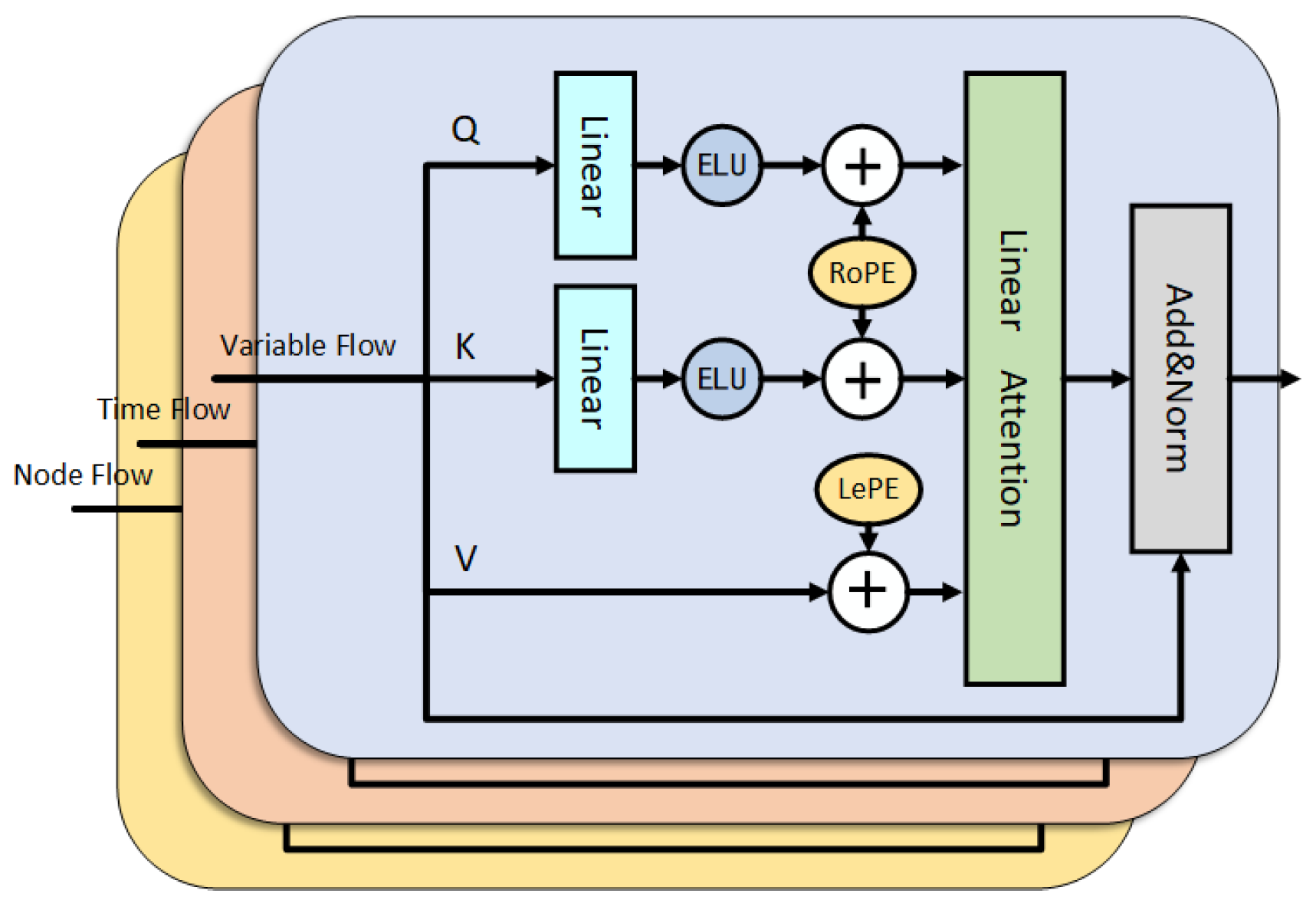
Variable-GCN, Time patch-GCN, and Node-GCN are followed by a linear attention encoder with rotational position encoding and local position encoding. The linear attention mechanism aims to reduce model complexity while learning global dependencies between variable sequences, within variable sequences, and between wind turbines, thereby improving the model’s representational capabilities. The detailed structure of the linear attention module is shown in Figure 2. The features learned by the dynamic graph convolution in Section 3.2 are used as the input of Q, K, and V. The query Q and key K are processed by the linear layer and then activated by the ELU function. The position information is then added to the query Q and key K through the rotation position encoding, and the local position encoding adds local spatial information to the value V, which supplements the deficiency of global dependency modeling in the attention mechanism [23]. After attention calculation, residual connection and layer normalization output are performed.

3.3.1. Variable Flow Attention Correlation

Linear attention mechanism [24,25] can effectively calculate the global correlation between variables and complete the weighted aggregation of features while reducing the complexity of the model. This is shown as follows:

$$E_G^V=\left\{\begin{array}{cccc}{E}_{G1}^{V1}& E_{G2}^{V1}& \dots & E_{GF}^{V1}\\ E_{G1}^{V2}& E_{G2}^{V2}& \dots & E_{GF}^{V2}\\ ⋮& ⋮& \ddots & ⋮\\ E_{G1}^{VN}& E_{G2}^{VN}& \dots & E_{GF}^{VN}\end{array}\right\}\to E_A^V=\left\{\begin{array}{cccc}{E}_{A1}^{V1}& E_{A2}^{V1}& \dots & E_{AF}^{V1}\\ E_{A1}^{V2}& E_{A2}^{V2}& \dots & E_{AF}^{V2}\\ ⋮& ⋮& \ddots & ⋮\\ E_{A1}^{VN}& E_{A2}^{VN}& \dots & E_{AF}^{VN}\end{array}\right\}$$

(27)

We update the feature $E_G^V$ learned from the Variable-GCN in Section 3.2.1 to $E_A^V$ through the linear attention mechanism. $E_{Ai}^{Vm}$ in Equation (28) represents the updated feature of the $i$th variable for wind turbine $m$, and $L_i^{Vm}$ represents the local position encoding of the $i$th variable for wind turbine $m$, which is learnable. $a_{ij}^m$ represents the relationship coefficient, which determines the amount of information each feature receives from other variables, as shown in Equation (29):

$$E_{Ai}^{Vm}={\displaystyle \sum _{j=1}^F{a}_{ij}^m}(W_v^{Vm}{E}_{Gi}^{Vm}+L_i^{Vm})$$

(28)

$$a_{ij}^m={\displaystyle \frac{\kappa (PoP{E}_i(W_q^{Vm}{E}_{Gi}^{Vm}))\kappa (PoP{E}_j(W_k^{Vm}{E}_{Gj}^{Vm}))}{{\displaystyle \sum _{j=1}^F\kappa (PoP{E}_i(W_q^{Vm}{E}_{Gi}^{Vm}))\kappa (PoP{E}_j(W_k^{Vm}{E}_{Gj}^{Vm}))}}}$$

(29)

In the above, $PoPE$ is the rotation position encoding, $\kappa$ is the kernel function ($ELU$), and $W_q^{Vm}$, $W_k^{Vm}$ and $W_v^{Vm}$ are learnable parameters.

3.3.2. Time Flow Attention Correlation

Linear attention mechanism can effectively calculate the global correlation between time slices while reducing model complexity, and thus performs weighted feature aggregation. This is calculated as follows:

$$E_{Ai}^{Tm}={\displaystyle \sum _{j=1}^P{a}_{ij}^m}(W_v^{Tm}{E}_{Gi}^{Tm}+L_i^{Tm})$$

(30)

In Equation (30), $E_{Ai}^{Tm}$ represents the updated feature for wind turbine $m$ at the $i$th time slice, and $L_i^{Tm}$ represents the local position encoding for wind turbine $m$ at the $i$th time slice. It helps the model capture short-term, high-frequency temporal dependencies, forcing the model to focus on the dependencies of these nearby moments and avoid being disturbed by irrelevant historical data in the long sequence. $a_{ij}^m$ represents the relationship coefficient, which determines the amount of information each feature receives from other time slices, as shown in Equation (31):

$$a_{ij}^m={\displaystyle \frac{\kappa (PoP{E}_i(W_q^{Tm}{E}_{Gi}^{Tm}))\kappa (PoP{E}_j(W_k^{Tm}{E}_{Gj}^{Tm}))}{{\displaystyle \sum _{j=1}^P\kappa (PoP{E}_i(W_q^{Tm}{E}_{Gi}^{Tm}))\kappa (PoP{E}_j(W_k^{Tm}{E}_{Gj}^{Tm}))}}}$$

(31)

In the above, $PoPE$ is the rotation position encoding, $\kappa$ is the kernel function ($ELU$), and $W_q^{Tm}$, $W_k^{Tm}$ and $W_v^{Tm}$ are learnable parameters.

3.3.3. Node Flow Attention Correlation

In the node flow, we still use linear attention mechanism, as shown below

$$E_{Ai}^{Nm}={\displaystyle \sum _{j=1}^N{a}_{ij}^m}(W_v^{Nm}{E}_{Gi}^{Nm}+L_i^{Nm})$$

(32)

In Equation (32), $E_{Ai}^{Nm}$ represents the updated feature of the $i$th wind turbine for environmental variable $m$, and $L_i^{Nm}$ represents the local position code of the $i$th wind turbine for environmental variable $m$. It can strengthen the close dependence between wind turbines, that is, the mutual influence of wind turbines at close distances is much stronger than that of wind turbines at far distances. $a_{ij}^m$ represents the relationship coefficient, which determines the amount of information each feature receives from other wind turbines, as shown in Equation (33):

$$a_{ij}^m={\displaystyle \frac{\kappa (PoP{E}_i(W_q^{Nm}{E}_{Gi}^{Nm}))\kappa (PoP{E}_j(W_k^{Nm}{E}_{Gj}^{Nm}))}{{\displaystyle \sum _{j=1}^N\kappa (PoP{E}_i(W_q^{Nm}{E}_{Gi}^{Nm}))\kappa (PoP{E}_j(W_k^{Nm}{E}_{Gj}^{Nm}))}}}$$

(33)

In the above, $PoPE$ is the rotation position encoding, $\kappa$ is the kernel function ($ELU$), and $W_q^{Nm}$, $W_k^{Nm}$ and $W_v^{Nm}$ are learnable parameters.

3.4. Fusion Prediction Module

After processing through the Triple-flow linear attention mechanism, we obtain features in three dimensions: variable, time, and node. The task of the feature fusion module is to fuse the features of these three dimensions to generate the final prediction result. Specifically, it uses a combination of splicing and fully connected layers to aggregate. Before feature splicing, it is necessary to map the features of each dimension to the same dimensional space through linear transformation to ensure the effectiveness of the splicing operation and the stability of subsequent feature fusion. Specifically, we convert the dimensions into: $E_A^V\in R^{N\times F\times D}\to R^{N\times D\times 1}$, $E_A^T\in R^{N\times F\times P\times D}\to R^{N\times D\times 1}$, $E_A^N\in R^{N\times F^{\prime }\times D}\to R^{N\times D\times 1}$. Then we concatenate the feature vectors along the second dimension through the concatenation operation, and $E_{cat}$ is the new feature after concatenation.

$$E_{cat}=Concat(E_A^V,E_A^T,E_A^N)\in R^{N\times 3D\times 1}$$

(34)

Finally, we map the hidden layer dimensions to the output time window dimensions through the fully connected layer to obtain the final prediction result:

$$E_{out}=E_{cat}{W}^{out}\in R^{N\times S^{\prime }\times 1}$$

(35)

On the one hand, this method retains the feature information of variable flow, time flow and node flow; on the other hand, it generates more expressive integrated features through the fully connected layer. These two aspects work together to effectively enhance the performance of the model.

3.5. Loss Function

TFDGCN uses mean square error (MSE) as our loss function, which is defined as follows:

$$Los{s}_{MSE}={\displaystyle \frac{1}{N\times S^{\prime }}}{\displaystyle \sum _{i=1}^N{\displaystyle \sum _{j=1}^{S^{\prime }}{(E_{out,i,j}-E_{True,i,j})}^2}}$$

(36)

where ETrue is the actual value of wind power, is $N$ the number of wind turbines, and $S^{\prime }$ is the size of the prediction time window.

4. Experiments

4.1. Data Description

We conduct experiments using the datasets SDWPF and SD23 obtained from two real wind farms. (1) SDWPF [26] is real wind power data from Longyuan Power Group. This dataset contains 4,727,520 records, sampled every 10 min, and collected over 245 days from a wind farm with 134 wind turbines. Each record contains 13 attributes, including environmental parameter features such as wind speed, wind direction, temperature and state features such as cabin temperature, cabin orientation. (2) The SD23 dataset. This dataset contains wind power data from a wind farm in Shandong Province, China. The dataset contains 2,170,800 records, sampled every 10 min, and covers 335 days of data from 45 wind turbines in the wind farm. The dataset spans from 1 January 2023 to 31 December 2023. Each record contains eight attributes, including features such as wind speed, yaw angle, and actual power.

For the SDWPF dataset, we used data from the past day to predict wind power for the next day. Specifically, we used the past 144 historical time windows to predict power for the next 144 time windows. We set the training, validation, and test sets to 155 days, 30 days, and 60 days, respectively. For SD23, we similarly used data from the past day to predict wind power for the next day. We split the dataset into 235 days, 67 days, and 33 days for training, validation, and testing, respectively.

Both of these datasets can be used for short-term, medium-term, and long-term forecasting tasks. The short-term time scale ranges from a few hours to a few days and is used for economic dispatch decisions, determining reserve requirements, and developing electricity market bidding strategies. The medium-term time scale ranges from a few days to a few weeks and is used for unit commitment and maintenance scheduling. The long-term time scale ranges from a few weeks to a few months, or even years, and is mainly used for wind power capacity planning and power system planning. Our task falls under short-term power forecasting.

For both datasets, the Top_k settings for the time flow, variable flow, and node stream were [8, 8, 8] and [8, 3, 8], respectively. The time slice length was 8. The feature dimension of the hidden layer was set to 128, and the number of heads was set to 2. The linear attention encoder dropout was set to 0.1, and the initial learning rate of the model was 1 × 10⁻⁴. The Adam optimizer was used to minimize the mean squared error (MSE) loss until training was terminated with an early stopping strategy. The model with the best performance on the validation set was selected as the final model and evaluated on the test set.

Table 1. Hyperparameters and their meanings.

Hyperparameters	Explain
patch_len	Length of time series patches in the time flow
dropout	Dropout probability, used to prevent model overfitting
n_heads	The number of heads in the attention mechanism
top_k	Number of nearest neighbors for constructing the adjacency matrix

shows the hyperparameters and their meanings

4.2. Evaluation Metrics

We use the mean absolute error (MAE) and root mean square error (RMSE) metrics to evaluate the performance of all methods on the entire wind farm. These two metrics are defined as follows:

$$MAE={\displaystyle \frac{1}{N}}{\displaystyle \sum _{i=1}^N\left|pre{d}_i-g{t}_i\right|}$$

(37)

$$RMSE={\displaystyle \sum _{i=1}^N\sqrt{\frac{1}{N}{\left(pre{d}_i-g{t}_i\right)}^2}}$$

(38)

where $N$ represents the number of wind turbines, $pre{d}_i$ represents the predicted value of wind turbine $i$, and $g{t}_i$ represents the actual value of wind turbine $i$. It is worth noting that SDWPF [26] provides a range for the abnormal values of the data, for example, the actual power must not be less than 0. If it is less than 0, it will be regarded as an abnormal value. Therefore, we will not use abnormal values or missing values for calculation and evaluation of the model.

4.3. Model Comparison

We compare the proposed TFDGCN with eight methods. These include four time series prediction models: LSTM [27], GRU [28], LSTM + Transformer [29], and TSAT [30], and four spatiotemporal prediction models: MTGNN [31], DCRNN [32], Bi-STAT [33], and AGCRN [34]. AGCRN and Bi-STAT are methods based on static graph networks. They take static graphs constructed based on Euclidean distance as input. MTGNN and DCRNN are based on the use of dynamic graph networks, where the adjacency relationships of graphs dynamically change over time. All parameters are set according to the data division in the previous section.

Table 2. Performance of different models on the SDWPF dataset.

Method	SDWPF
	MAE (MW)	RMSE (MW)
LSTM	41.23	46.15
GRU	40.92	46.40
LSTM + Transformer	39.21	46.32
TSAT	38.03	44.91
AGCRN	38.45	45.92
Bi-STAT	38.34	45.75
MTGNN	40.43	46.61
DCRNN	38.33	46.52
TFDGCN	37.16	44.84

and

Table 3. Performance of different models on the SD23 dataset.

Method	SD23
	MAE (MW)	RMSE (MW)
LSTM	15.94	17.73
GRU	16.38	18.03
LSTM + Transformer	15.58	17.63
TSAT	15.27	17.79
AGCRN	15.81	17.83
Bi-STAT	15.63	17.82
MTGNN	15.37	17.65
DCRNN	15.49	17.75
TFDGCN	14.63	17.56

respectively present the performance of all models on the SDWPF dataset and SD23 dataset. Based on the results shown in Table 2 and Table 3, it can be observed that the proposed TFDGCN performs well in both MAE and RMSE metrics, indicating that the model has good generalization and predictive performance. From Table 2, it can be found that the prediction accuracy of spatiotemporal models (AGCRN, Bi-STAT, MTGNN, DCRNN) is superior to traditional temporal models (LSTM, GRU, and LSTM + Transformer). This indicates that spatiotemporal models can more comprehensively capture the complex patterns of wind power data by integrating temporal and spatial information, thus outperforming temporal models in prediction accuracy and generalization ability. From Table 3, it can be seen that the prediction accuracy of spatiotemporal models based on dynamic graphs (MTGNN, DCRNN) is better than that of spatiotemporal models based on static graphs (AGCRN, Bi-STAT). This indicates that dynamic graphs can better capture the spatiotemporal dependencies that vary over time in wind farms.

To further evaluate the model we proposed, we visualized the prediction results of TFDGCN on SDWPF dataset. We summed the wind power of all turbines from 4–5 August 2023, to obtain the total power of the wind farm, and plotted it together with the TFDGCN predictions for the same time period. Figure 3 shows the error between the predicted and actual power.

4.4. Research on Top-k Values

We conducted experiments on the selection of the Top_k parameter for the variable flow, time flow, and node flow of TFDGCN using two datasets. In the experiments, we fixed the Top_k values of two of the flows to investigate the impact of the Top_k value of the remaining flow on model performance. On the SDWPF dataset, when the Top_k values of the variable flow and temporal flow were fixed, the effects of changes in the Top_k value of the node flow on MAE and RMSE are illustrated in Figure 4a,b. On the SD23 dataset, when the Top_k values of the variable flow and temporal flow were fixed, the effects of changes in the Top_k value of the node flow on MAE and RMSE are shown in Figure 4c,d. As presented in Figure 4, regardless of the dataset, both MAE and RMSE first decrease and then increase as Top_k increases. Specifically, as shown in Figure 4a–c, the optimal Top_k value is 8. This indicates that: A lower Top_k value means a smaller number of neighbors, resulting in limited information aggregated by the graph convolution operation from neighboring nodes. A higher Top_k value implies a larger number of neighbors; during the aggregation process of graph convolution, the model will be affected by neighbors irrelevant to the target node. Such irrelevant neighbors interfere with the model’s learning and reduce its wind power prediction performance. We also conducted experiments on the Top_k values of the variable flow and temporal flow using the same method. On the SD23 dataset, the impact of changes in Top-k values of variable flows and temporal flow on MAE and RMSE are shown in Figure 5a,b and Figure 6a,b, respectively. Based on the experimental results, the Top_k values for the temporal flow, variable flow, and node flow were all set to 8.

4.5. Ablation Studies

4.5.1. Studies on the Validity Ablation of Triple-Flow Structure

To assess the effectiveness of the triple flow architecture of TFDGCN, we compared it with three other architectures, where the definitions of the comparative architectures are as follows: T&N denotes the structure that removes the variable flow while retaining the temporal flow and node flow. T&V denotes the structure that removes the node flow while retaining the temporal flow and variable flow. T&V&StaticN denotes the three-branch structure that replaces the dynamic graph of the node flow with a static graph based on Euclidean distance. The results are presented in

Table 4. Ablation study of the effectiveness of the triple flow structure.

Method	SDWPF		SD23
	MAE	RMSE	MAE	RMSE
TFDGCN (T&V)	37.56	45.49	14.86	17.59
TFDGCN (T&N)	37.88	45.32	15.23	17.61
TFDGCN (T&V&StaticN)	37.35	44.93	14.75	17.63
TFDGCN	37.16	44.84	14.63	17.56

. It can be observed that removing the variable flow, removing the node flow, or using a static graph all lead to a decline in model performance. Specifically, the MAE of T&N and T&V is 1.9% and 1% higher than that of TFDGCN, respectively. This indicates that both the variable flow and node flow contribute to improving the performance of TFDGCN. Additionally, T&V&StaticN performs worse than TFDGCN, which demonstrates the role of dynamic graphs in enhancing the performance of TFDGCN.

4.5.2. Ablation Study on the Effectiveness of Attention Mechanism

We removed the linear attention module of TFDGCN, and the experimental results are shown in

Table 5. Ablation study on the effectiveness of attention mechanism.

Method	SDWPF		SD23
	MAE	RMSE	MAE	RMSE
Delete Attention	38.87	44.86	14.98	17.63
TFDGCN	37.16	44.84	14.63	17.56

. It can be seen that removing the linear attention module has an impact on the model’s prediction performance. This indicates that the linear attention module can effectively capture global dependencies and contributes to the performance of TFDGCN.

To verify the advantage of linear attention mechanism in inference time, we compared the inference time of applying linear attention mechanism and global attention mechanism in TFDGCN. We conducted this experiment on 60 batches of data spanning from day 185 to day 245. Each batch contains daily monitoring data for 134 fans, including 13 fields. We can see from

Table 6. Inference time.

Method	Average Inference Time	Total Inference Time
TFDGCN (LinearAttention)	26.685 ms	1574.421 ms
TFDGCN (GlobalAttention)	41.168 ms	2428.925 ms

that the linear attention mechanism encoder outperforms the global attention mechanism encoder in inference time.

5. Conclusions

We propose TFDGCN, a novel spatiotemporal wind power short-term prediction model. TFDGCN has a three-branch structure, which models the variable dimension, time dimension, and node dimension separately to capture heterogeneous dependencies in spatiotemporal sequence data. Experimental results show that the proposed TFDGCN outperforms traditional temporal models and the state-of-the-art method in terms of performance. The ablation experiments further confirmed the effectiveness of the three-branch structure, that is, when any one of the three branch structures is removed, the model performance decreases. Removing the linear attention module will also result in a decrease in prediction accuracy. This demonstrates the role of the linear attention mechanism in extracting global dependencies.

The latest research results show that the collaborative application of wind power prediction and power scheduling optimization can improve the quality of scheduling strategies. In future work, we will attempt to study the synergistic effect between wind power forecasting and power dispatch optimization, in order to further reduce the operating costs of the power grid and ensure the safe and stable operation of the power system.