PGF-Net: A Symmetric Cutting Path Generation and Fitting Optimization Method for Pig Carcasses Under Multi-Medium Interference

Abstract

In the automated cutting process of pork carcasses, asymmetric cutting path planning is critical. However, various substances on the carcass surface, such as blood stains and fascia, severely interfere with the separation boundaries between fresh meat and bones, significantly reducing the accuracy of asymmetric cutting path planning. To address these issues, this paper proposes a method for generating and fitting optimized cutting paths for pork carcasses (PGF-Net). Specifically, this method comprises a cutting path generation module that integrates multi-scale boundary features and a cutting path fitting optimization module. The cutting path generation module extracts asymmetric boundary information by enhancing attention to boundaries across different regions, identifies key cutting points, and generates a coarse cutting path. The cutting path fitting optimization module then performs fitting optimization on the generated key cutting points to ultimately produce a refined asymmetric cutting path. Experimental results demonstrate that PGF-Net achieves mean root mean square errors of 0.4212 cm, 0.4651 cm, and 0.5313 cm across three cutting paths on six different pork carcass images. Findings confirm that this method enhances the yield of premium meat cuts while reducing tool wear costs. It provides an innovative technological solution for automated meat processing, holding significant industrial application value.

1. Introduction

With the annual growth rate of global meat consumption continuing to climb, technological innovation in pork carcass cutting, a core process in the meat processing industry chain, has become increasingly critical. As industrial intelligence advances, traditional semi-automated pork carcass cutting equipment reliant on manual labor suffers from inefficiencies, inconsistent cutting standards, cross-contamination risks, and high meat waste rates [1]. The meat cutting industry is characterized by harsh working conditions and heavy workloads, leading to labor shortages. Consequently, novel automated methods are urgently needed to address these challenges [2]. Precise asymmetric cutting path generation forms the foundation for automated cutting. Current research primarily employs machine vision and deep learning technologies, yet significant challenges remain [3]. Current research on pork carcass cutting path generation primarily employs machine vision systems or neural networks, though these approaches exhibit limitations. Even with progress in initial path generation, direct application to actual cutting remains inadequate. While fitting optimization in cutting path research has focused on autonomous driving and trajectory correction, referencing these methods remains crucial. This paper reviews relevant work from two perspectives: cutting path generation and fitting optimization.

In terms of asymmetric cutting path generation, the primary methods currently include image segmentation and convolutional neural networks. Nisbet et al. [4] introduced a machine vision system to the inspection of critical parts of cattle carcasses, which accurately delineated the parts and verified the errors by using RMSE through the 3D image data of cattle carcasses. Fernandes et al. [5] introduced machine vision as well as a method to predict pig weight, pig lean, and pig back fat using 3D images to measure pig biometrics and weight. Machine vision is the basis for automation, which uses image processing technology to automate the discrimination of cutting parts of pig carcasses, segmenting the key parts of pig carcasses, and the planning of cutting paths between the parts is key. Lu et al. [6] used an improved three-level color machine vision algorithm, which segments the parts of the chicken through color analysis, contour extraction, and pose matching. Yu et al. [7] used the DeepLab+ResNet50 model because of the distinct boundary between the fatty and lean parts of the meat, which segmented the longest muscle region of the back after correcting for image distortion and chromatic aberration. Cong et al. [8] designed a binocular vision-based robotic system for cutting pig abdomen, using threshold segmentation to detect the contour of pig carcasses, based on the contour using principal component analysis to determine the position of the cutting line. Finally, a binocular vision camera is used to complete the depth extraction of the center line, which is used to guide the robot to adjust the cutting path. Afonso et al. [9] proposed a prediction model for the segmentation of lamb carcass tissues, which selects six characteristic points (center, center of mass, and four vertex coordinates) of the minimum outer connecting rectangle of the four sites with respect to the positional relationships of muscle, subcutaneous fat, intermuscular fat, and bone. However, lamb carcass morphology is complex and variable, and image processing is poorly adapted with low prediction accuracy. In cases where the cutting boundary is clear and the contour of the area is distinct, the above cutting methods can be used for meat processing. However, it is less applicable in pig carcass cutting tasks with large body size differences, ambiguous boundary information, cross-mixing of bone and meat media, and complex cutting paths.

The hierarchical feature extraction mechanism and local perceptual characteristics unique to convolutional neural networks enable deep learning-based image processing algorithms to achieve high precision when performing pixel-level object segmentation tasks [10]. Zhao et al. [11] proposed a real-time semantic segmentation method for sheep carcasses, which achieves accurate segmentation of three parts of sheep carcasses. Tran et al. [12] proposed a poultry carcass cutting method based on the framework of an end-to-end converter, which accurately realized the segmentation of each part region of the poultry carcass. However, it did not improve the structure of the segmentation network itself, and there is still a lot of room for improvement in segmentation accuracy. Ban et al. [13] innovatively introduced a semantic segmentation neural network to the task of cutting pig carcasses, realizing the cutting of key parts of the spine ribs of pig carcasses. Liu et al. [14] proposed a laser-guided efficient cutting path planning method, which combines a segmentation algorithm (SA) with an improved genetic algorithm (GA), and finally identifies the cutting path of pork belly from the 3-D laser point cloud data of pig carcasses. Bao et al. [15] studied the characteristics of sheep carcass profile structure and the mechanical properties of sheep meat and sheep ribs, constructed a three-dimensional model of sheep carcass, and constructed a dynamic model of the slaughtering robot. Finally, the planning of the sheep carcass cutting path was completed from the perspective of mathematical modeling. Bu et al. [16] proposed a laser scanner-based 3D point cloud method for cutting pork pancetta, hind leg and tenderloin and obtaining meat contour information by constructing a contour adaptive shaping unit. Niu and Cai [17] proposed a cutting line construction method for the muscle tissue of pig carcasses, which is based on blurred and distorted X-ray images, using a convolutional neural network to extract the X-ray image features and correcting the muscle and bone edge information. Finally, the segmentation contour information was utilized to obtain the cutting line. Liu et al. [18] proposed a new real-time pork belly cutting path planning method. By using laser sensors instead of traditional machine vision, 3D laser point cloud data of pig carcasses are acquired, and the 3D point cloud data are downscaled and cutting paths are planned using the image pyramid method. Balkrishna et al. [19] constructed a 3D model of the data obtained after CT scanning and aligned it with the point cloud data taken by the camera. Cutting paths were generated on the surface of the 3D model, taking into account the skeletal structure of the pig carcass and the cutting characteristics of the tool. The above studies realized semantic segmentation of key parts of carcasses, and in planning cutting paths for pig carcasses, they are still stuck in relying on machine vision and positional characteristics between key parts to determine cutting paths. Moreover, the pig carcass surface suffers from media cross-mixing and a complex background, and the applicability of the cutting path generation method has not been verified.

With regard to asymmetric cutting path fitting optimization, Wang and Cai [20] proposed a meta-learning based cutting force follow-shape regulation method, which constructs a reinforcement learning-based tool follow-shape regulation model during the cutting of pig carcasses, obtains the optimal action sequences, and achieves the optimization of the cutting path from the feedback information of the tool. Yang et al. [21] proposed a visual navigation path extraction method based on neural networks and pixel scanning. The semantic segmentation network was trained based on Segnet and Unet, and the designed scanning method, filtering algorithm, and weighted average method were used to fit the navigation paths. Zheng et al. [22] proposed an improved lightweight YOLOX-Nano architecture to detect the fruit tree root points and applied the K-means clustering algorithm to classify the root points into two categories belonging to the left and right tree rows and to determine the navigation paths through geometric relationships and least squares. Yu et al. [23] proposed a new method for training Bessel curve control points using radial basis function neural networks, where initial paths are planned by the arc-line-arc three-segment composite curve, and five-times Bessel curve fitting is used to compensate for curvature discontinuities. Dai et al. [24] proposed an online trajectory optimization method for hypersonic vehicles based on convex programming and feedforward neural networks. The feedforward neural network is trained based on multiple optimal trajectories generated offline under aerodynamic uncertainties, and the optimal trajectories are output in real time. Molina-Leal et al. [25] applied a Long Short-Term Memory neural network network (LSTM) to learn the mapping between inputs and outputs in sample data, which can obtain the linear and angular velocities of the mobile robot. This allows the mobile robot to find the optimal trajectory between two points. Lin et al. [26] combined TTCN, the attention mechanism, and GRU network to construct a hybrid model for ship trajectory prediction, where the attention mechanism can better help the neural network to learn the data features, and the GRU has a strong nonlinear fitting ability, which can achieve the fitting optimization of the ship trajectory. In general, time series-based neural networks can be well applied in the field of pig carcass cutting. It can achieve the fitting optimization of the cutting path according to the horizontal and vertical coordinates of the cutting path, the initial direction, and the cutting speed. The optimal cutting path is obtained while ensuring compliance with the cutting criteria.

Therefore, the aim of this paper is to solve the problem of generating and optimizing asymmetric cutting paths for critical parts in the complex context of pig carcasses. An cutting path generation and fitting optimization method for pig carcasses under multi-medium interference (PGF-Net) was proposed. The accuracy of the cutting path has been validated according to current standards. The main contributions of this method are as follows:

• We developed a cutting path generation method (CGM) that integrates a multi-scale boundary feature extraction module (MBM). This module extracts and fuses boundary information across multiple scales to generate effective cutting paths between key components;
• We propose a bifurcated cutting path fitting module (BFM). This module performs fitting optimization on the generated cutting paths based on information such as the horizontal and vertical coordinates of the cutting position, as well as the speed and direction of the cutting tool.

2. Materials and Methods

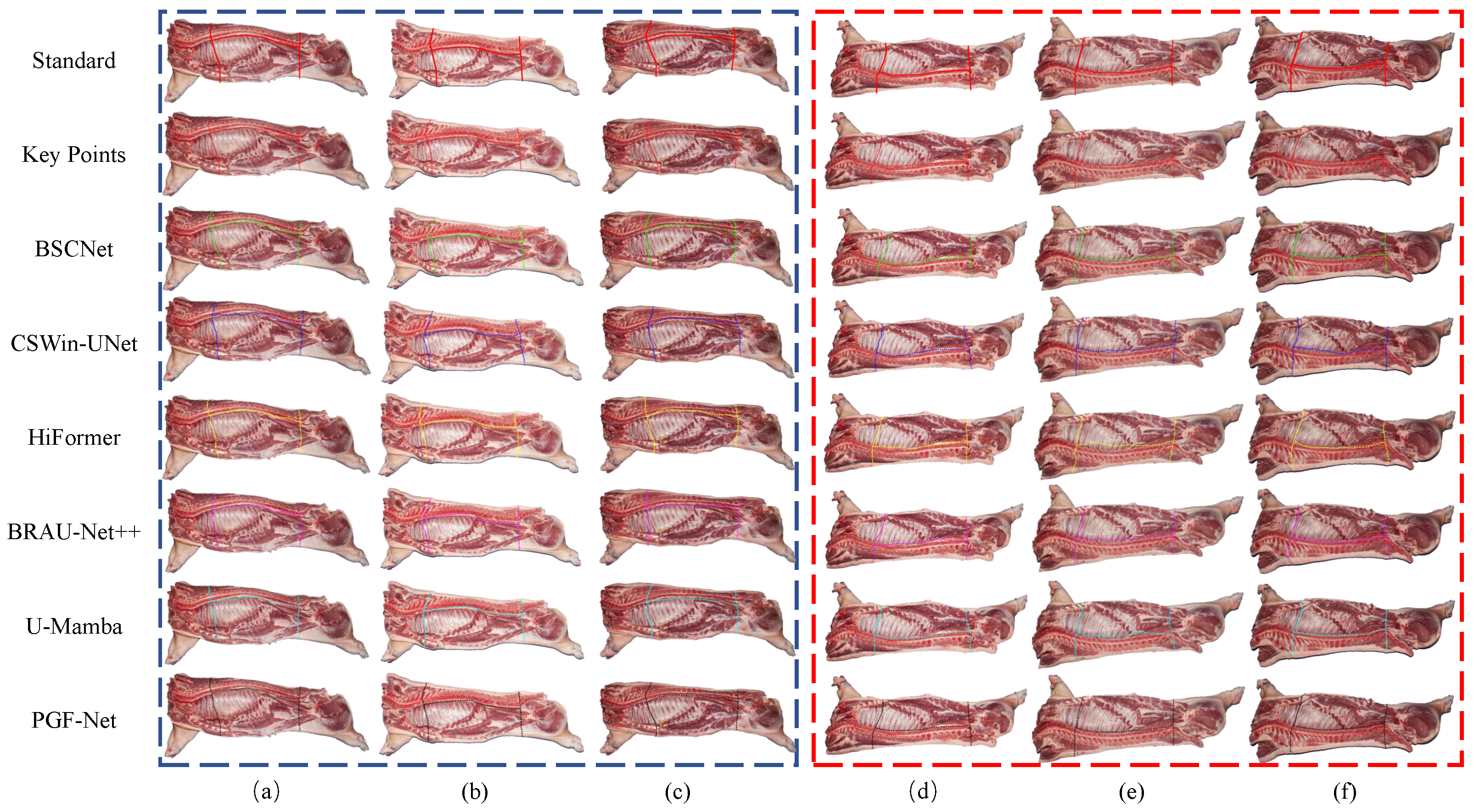
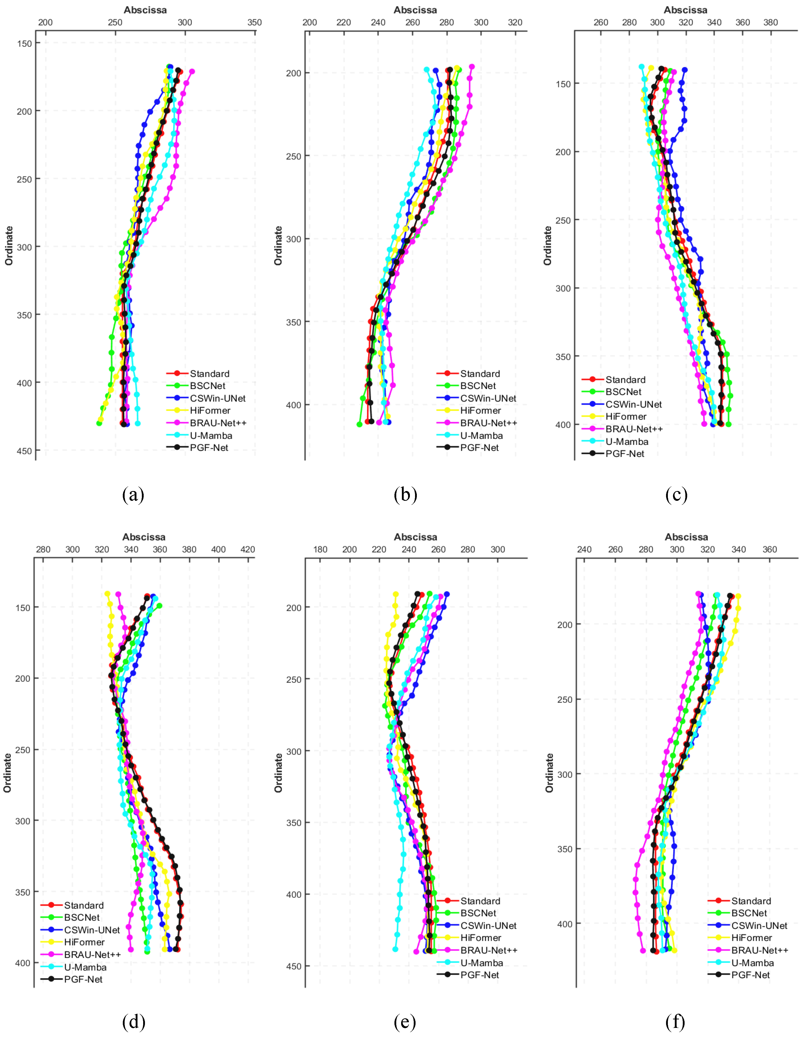
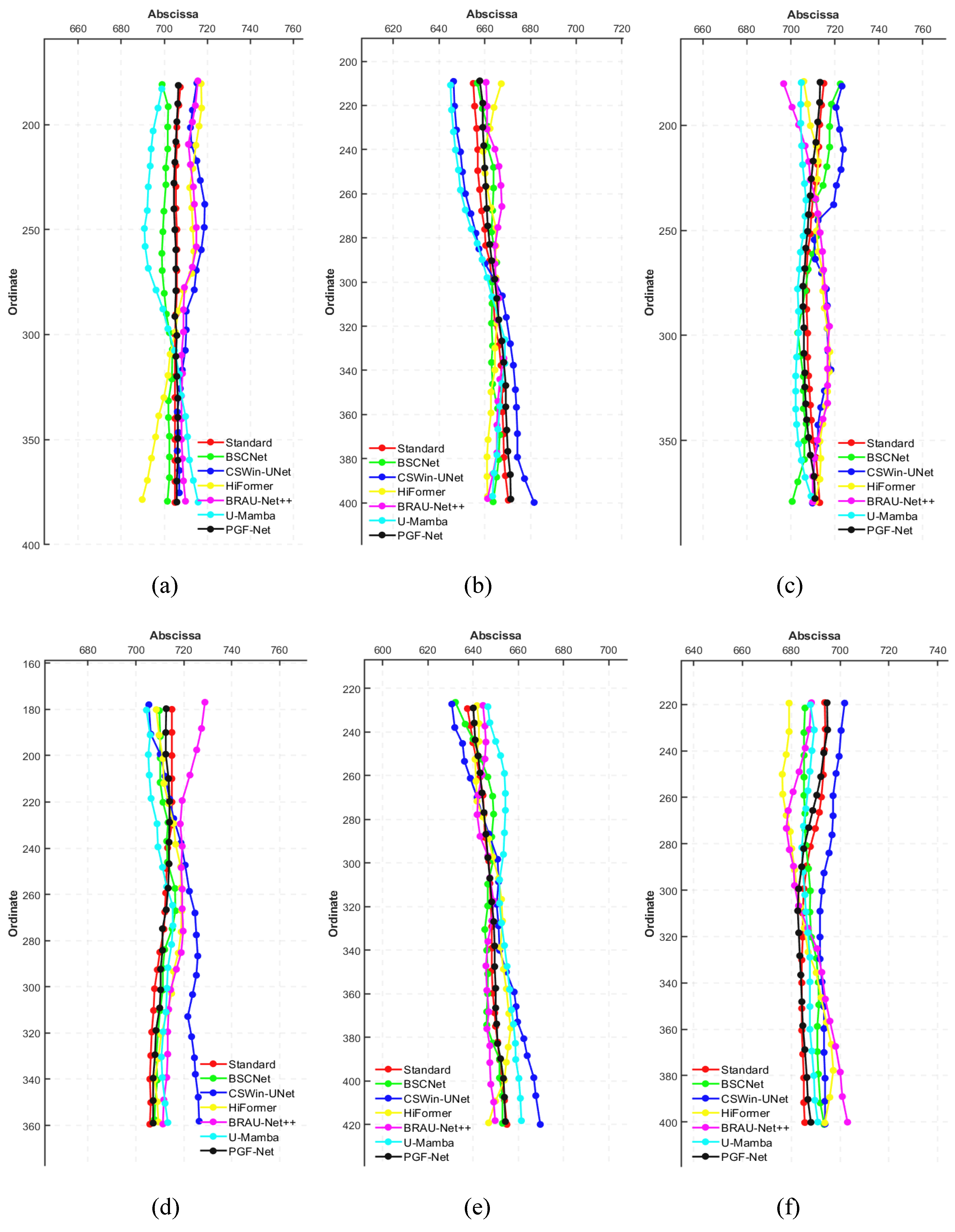
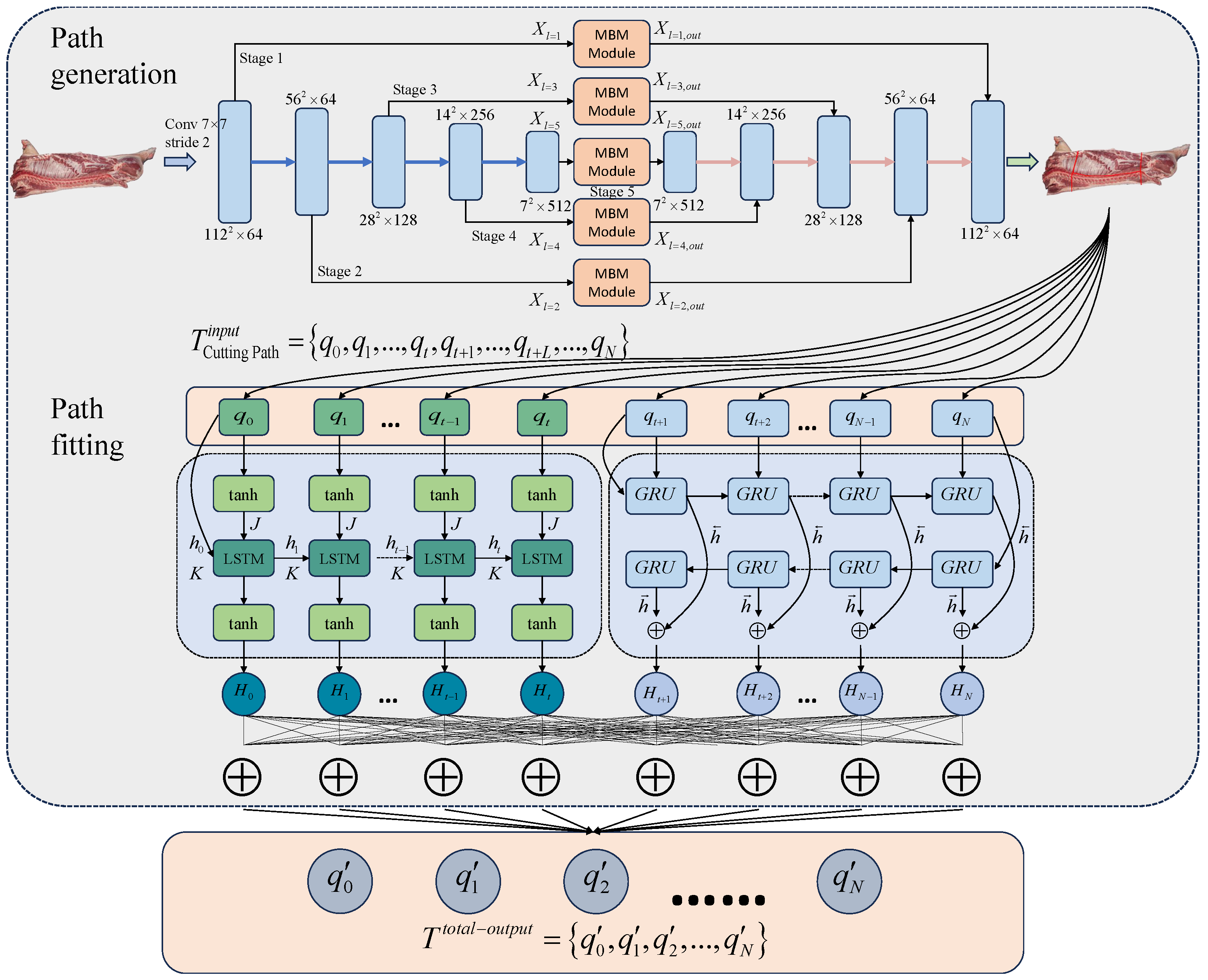
In this section, a generation and fitting optimization method for pig carcass cutting paths (PGF-Net) is described in detail. First, the boundary constraint cutting path generation method (CGM) is introduced as a whole. Then, the main structure of the multi-scale boundary extraction module (MBM) and the realization principle are explained. Finally, a bifurcated cutting path fitting module (BFM) is proposed, and the recursive network of two branches and the implementation process are described in detail. The network framework of the algorithm in this paper is shown in Figure 1.

2.1. Cutting Path Generation Method (CGM)

In this section, a rough generation method for pig carcass cutting paths is proposed, as shown in Figure 2. The method mainly uses semantic segmentation to obtain the cutting boundary. First, a convolution operation with a step size of 2 is performed on the input image. Then, it is inputted into the rough path generation network, and the convolution operation with 5 different stages is performed. The image after the convolution of each scale is input into the multi-scale boundary extraction module separately to enhance the extraction of boundary features. The residual linking mechanism is used, which mainly consists of two $3\times 3$ convolution blocks and feature summation to avoid gradient vanishing. In each multi-scale boundary extraction module, it is divided into five scales after a $3\times 3$ DW convolution, and then DW convolution is performed for each of the five scales. The final feature fusion is performed to recover the original size of the image by a $1\times 1$ convolution. The enhanced target features from the multi-scale boundary extraction module are fused with the corresponding scale decoding blocks, and then richer boundary detail information is obtained.

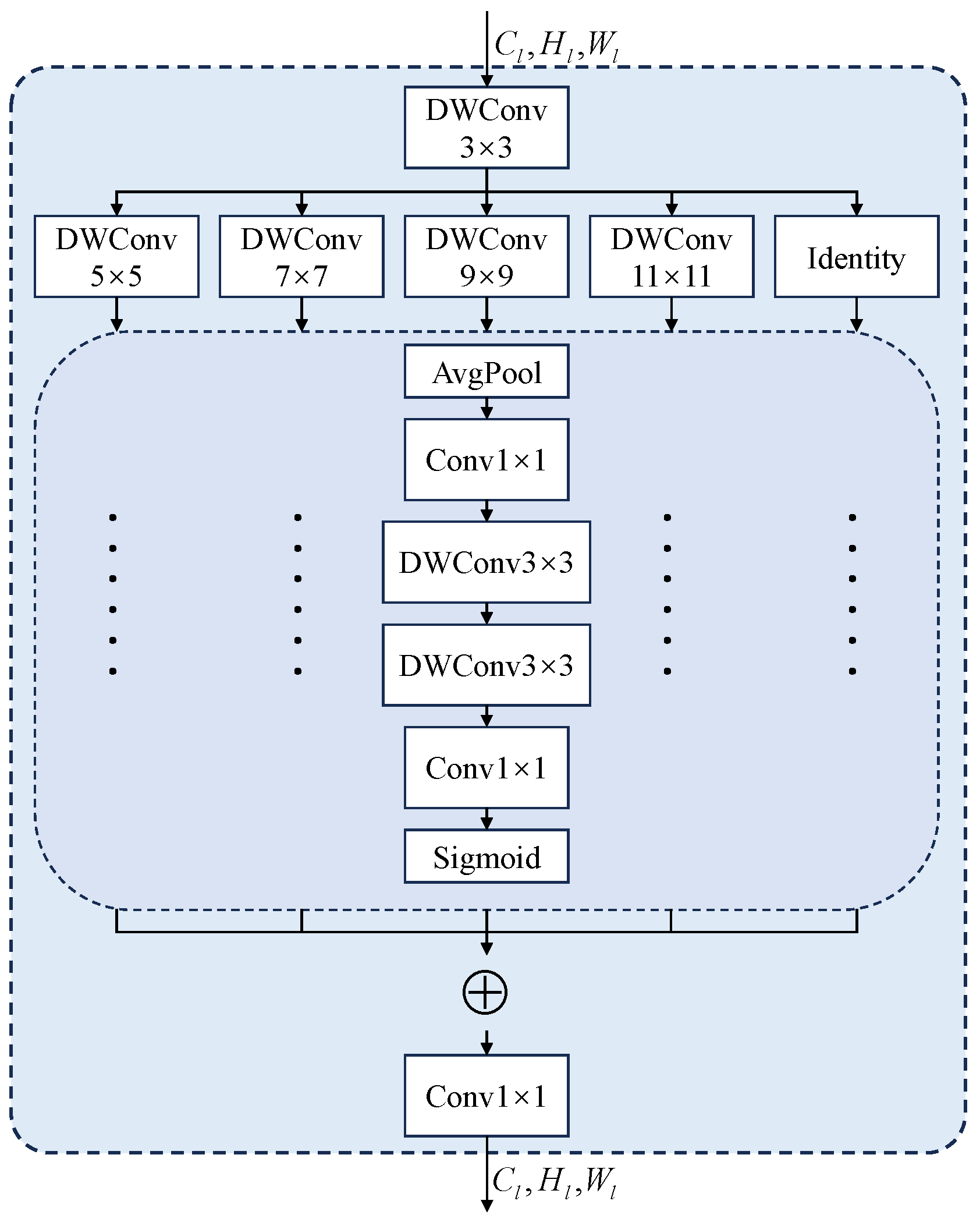
During the cutting process of pig carcasses, the images have problems such as large body size differences, blood stains at critical parts, and missing boundary information due to fascia coverage. In this paper, the MBM module is introduced to capture the multi-scale information of the key part features, and the MBM module is shown in Figure 3. The MBM module includes a small kernel convolution to capture the local information. Then, there is a set of parallel deep convolutions to capture the contextual information on multiple scales, where an Identity block is set to ensure the consistency of the feature information. The n th MBM block in stage l is represented by the following equation:

$$L_{l,n}=Con{v}_{k_s\times k_s}\left(X_{l,n}\right),(n=1,\dots ,5,s=5,7,9,11,13),$$

(1)

$$Z_{l,n}=DWCon{v}_{k^{\left(n\right)}\times k^{\left(n\right)}}\left(L_{l,n}\right),(n=1,\dots ,4),$$

(2)

where $L_{l,n}\in {\mathbb{R}}^{C_l\times H_l\times W_l}$ is the localized feature extracted through $k_s\times k_s$. $Z_{l,n}\in {\mathbb{R}}^{C_l\times H_l\times W_l}$ is the contextual feature extracted by the n th $k^{\left(n\right)}\times k^{\left(n\right)}$ deep convolution $\left(\mathrm{DWConv}\right)$. In this experiment, the settings n and s correspond to each branch. As an the example, in the n th branch of the l th stage, average pooling is used first. Then, a $1\times 1$ convolution is performed to obtain the local region features. It can be represented as

$$F_{l,n}^{pool}=Con{v}_{1\times 1}\left(P_{avg}\left(X_{l,n}\right)\right),(n=1,\dots ,5),$$

(3)

where $P_{avg}$ denotes the average pooling operation. Then, two depth strip convolutions are applied as an approximation to the standard large kernel depth convolution. It can be represented as

$$F_{l,n}^w=DWCon{v}_{1\times k_b}\left(F_{l,n}^{pool}\right),$$

(4)

$$F_{l,n}^h=DWCon{v}_{k_b\times 1}\left(F_{l,n}^w\right).$$

(5)

Deep strip convolution is chosen based on two main factors. First, strip convolution is lightweight. A similar effect is achieved with a pair of 1D deep kernels with ${\displaystyle \frac{k_b}{2}}$ fewer parameters compared to the traditional $k_b\times k_b$ 2D deep convolution. Secondly, strip convolution can be better extracted for feature recognition and extraction of the thin strips (e.g., loin). In order to adapt to different sensory fields and better extract multi-scale features, $k_b=5,7,9,11,13$ is set so that it can obtain more relevant semantic linkage of feature information in the feature extraction process. And the design of strip convolution can avoid the increase in computational cost to some extent. Finally, an attention weight $A_{l,n}\in {\mathbb{R}}^{{\displaystyle \frac{1}{2}}{C}_l\times H_l\times W_l}$ is generated to further enhance the output of the MBM module. This is expressed by the following equation:

$$A_{l,n}=Sigmoid\left(Con{v}_{1\times 1}\left(F_{l,n}^h\right)\right),$$

(6)

where the $Sigmoid$ function is to ensure that the attention graph $A_{l,n}$ stays within the $\left(0,1\right)$ range. $A_{l,n}$ is the output of the entire module at the n th branch of the l th stage. The output of the entire module is

$$X_{l,out}=Con{v}_{1\times 1}\left({\displaystyle {\sum }_1^5}{A}_{l,n}\right)\left(l=1,\dots ,5\right),$$

(7)

where $X_{l,out}$ is the feature that has been enhanced by the module.

2.2. Bifurcated Cutting Path Fitting Module (BFM)

In this section, a double-ended GRU bifurcated cutting path fitting optimization model (BFM) based on forward and backward recurrent networks is proposed, and the overall network structure is shown in Figure 4. The framework is divided into three parts. (1) The sequence of cutting path key points extracted from the CGM module as input data. (2) A bidirectional linear regression network layer. (3) A fusion output layer that aggregates data from the two-branch network. The main components include input data preprocessing, a dual-branch network, and summation and fusion output. Data preprocessing operates on raw, actual coarse segmentation path data. Through data integration techniques, the fusion status information of key segmentation points is converted into a sequence of segmentation paths. The forward recursive network starts from the cutting origin point, extracting features based on adjacent feature information. The backward recursive network begins at the cutting endpoint, extracting features based on adjacent feature information. Each recursive network separately fits the input cutting path sequence. Finally, the fusion layer outputs the sequence of fitted cutting path points by summing the features. In the BFM module, the cutting path fitting problem can be expressed as an optimization problem, whose objective is to minimize the error between the predicted path and the actual path. We define the objective function as

$$MSE=\underset{\theta }{min}\sum _{t=1}^T{∥{\widehat{y}}_t-y_t∥}^2,$$

(8)

where ${\widehat{y}}_t$ is the predicted output of the model at time t, $y_t$ is the true cut waypoint, and $\theta$ is the model parameter. By optimizing this objective function, the BFM module can fit the cutting path more accurately.

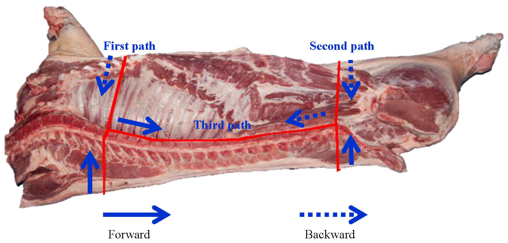
The rough cutting path generated by the pig carcass cutting path generation method, which only has RGB image information, needs to be preprocessed before inputting it to the cutting path fitting optimization algorithm, as shown in Figure 5. The preset cutting paths are set as three paths with known state data as the first path, the second path, and the third path. The existing three paths are just a collection of points on the RGB image, and the horizontal coordinates, vertical coordinates, movement speed, direction of travel, and relative time at moment t of the cutting device during the cutting process need to be fused. The position information of the cutting tool at moment t can be represented as $q_t=\left\{ab{s}_t,or{d}_t,ve{l}_t,po{s}_t,tim{e}_t\right\}$. Where $ab{s}_t$, $or{d}_t$, $ve{l}_t$, $po{s}_t$, and $tim{e}_t$ are the horizontal coordinates of the corresponding cutting position, the vertical coordinates, the cutting tool moving speed, the direction of travel of the cutting tool, and the relative time at the moment of t, respectively.

In the cutting process, the feed point and the cutting direction of the front section are extremely important; it requires the forward network to have a good ability to deal with complex long sequences. Therefore, a standard LSTM network is used as the forward network. The pig carcass cutting path data with moments from 0 to t are organized into a data vector $T_{Forward}^{LSTM-input}=\left\{{q_0}^{*},{q_1}^{*},\dots ,{q_t}^{*}\right\}$, which is used as the input vector of the forward network. The hidden layer is $h=\left\{h_0,h_1,h_2,\dots ,h_t\right\}$. The forward network takes the computed cell state and outputs and combines them to form the state vector $H=\left\{H_0,H_1,H_2\dots ,H_t\right\}$. Then, J, K, and S denote the values of the layer-to-layer weighting metrics, respectively. The hidden and output layers can be represented as

$$h_i=\left\{\begin{array}{c}tanh\left(J{q}_i+b_i^h\right)whilei=0\hfill \\ tanh\left(J{q}_i+K{h}_{i-1}+b_i^h\right)whilei=1,2,3,\dots ,t\hfill \end{array}\right.,$$

(9)

where $q_i$ denotes the state data at moment $t=i$. $b_i^h$ and $b_i^H$ denote the bias values of the hidden and output layers, respectively.

LSTM is able to recognize long-term data better than traditional RNN networks. LSTM solves the problem of long term dependence of data, thanks to the setup and effective cooperation of its input gates, forgetting gates, output gates, and cell state, defined as i, f, o, and c, respectively. Among them, the forgetting gate will decide which cut path point data need to be retained after receiving the previous state data, mainly realizing the filtering of abnormal path point interference. The input gate determines which data need to be retained and updates the cell state. The output gate is what controls which information from the current time step is transferred to the next or output layer. The cell state is the core of the whole network, which can store and transfer information, as well as control the flow and update of information.

The purpose of the forgetting gate is to minimize the interference of anomalous path points on subsequent fitted cut paths, in addition to being responsible for the collection of data from the previous moment. Then, the recursive input $h_{t-1}$ and the current input $q_t$ are multiplied by their weights as inputs to the $Sigmoid$ function denoted as $\sigma \left(q\right)={(1+e^{-q})}^{-1}$. If output $f_t$ is a value within $\left[0,1\right]$, multiply by cell state $c_{t-1}$. If $f_t$ outputs 1, the LSTM will save this new data, and if $f_t$ outputs 0, the LSTM will completely forget this data.

$$f_t=\sigma \left(J_f{q}_t+K_f{h}_{t-1}+b_f\right).$$

(10)

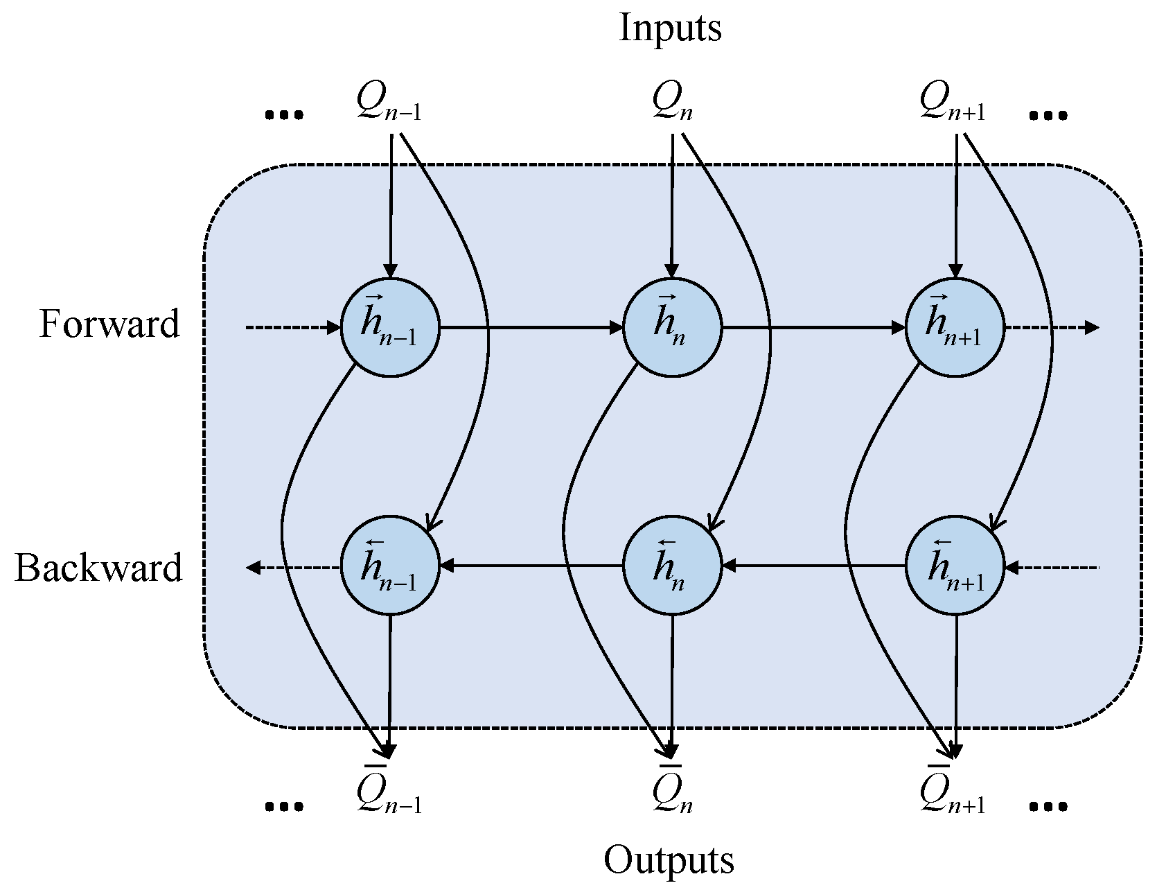
In order to synthesize the efficiency and accuracy of the cut-path fitting, the backward recurrent network that is chosen ensures the correlation between the previous and subsequent moments and at the same time ensures the efficiency of the data sequence processing. In this section, a two-headed GRU network is chosen to realize the fitting of the path from $q_{t+1}$ to $q_N$. The cut path data sequence has the single data characteristics of incremental time information, detailed path information, and small fluctuations between neighboring path points. These data characteristics can better meet the requirements of GRU to handle long data sequences, thus ensuring that the Sigmoid function in the update gate is in an intermediate state distribution. The training effect of each input data is maximized, thus reducing the gradient vanishing and improving the accuracy of path fitting. In this paper, the input cut path vector $T_{Backward}^{BiGRU-input}=\left\{{q_{t+1}}^{*},\dots ,{q_{N-1}}^{*},{q_N}^{*}\right\}$, after bi-directional GRU computation as well as summing, outputs the combined state vector $H=\left\{H_{t+1},H_{t+2},\dots ,H_N\right\}$.

The update gate is updated based on the $abs$ and $ord$ fields in the cut path data. When the two data changes are small, the curvature of the cutting path changes are relatively small, then the update gate takes a smaller value close to 0, and the weights should also take a smaller value. The equation is expressed as follows:

$$z_N=tanh\left(W_z·\left[h_{N-1},{q_N}^{*}\right]\right),$$

(11)

where $W_z$ denotes the weight of the update gate. $h_{N-1}$ is the state at the time of the previous path point. tanh takes values between −1 and 1.

The purpose of the reset gate is to minimize the interference of anomalous path points with subsequent fitted path points. When the reset gate takes a value close to 1, it means that the state values should be invalidated and discarded, thus ensuring the accuracy of the cut path fitting. The expression for the reset gate is shown below.

$$r_N=tanh\left(W_r·\left[h_{N-1},{q_N}^{*}\right]\right),$$

(12)

where $W_r$ is the weight belonging to the reset gate. $h_{N-1}$ is the state of the previous path point. tanh takes values between −1 and 1.

The output variable $h_N$ denotes the output vector value of this network model at moment N. Variable ${\tilde{h}}_N$ denotes the degree of dependency between the candidate state at the current moment and the cut path state value at the previous moment. $h_N$ is responsible for storing the position, attitude direction, and velocity information of the cutting path, and it serves as an input variable for the next moment. The equation is expressed as follows:

$${\tilde{h}}_N=tanh\left(W_h{q_N}^{*}+U_h\left(r_N\otimes h_{N-1}\right)+b_h\right),$$

(13)

$$h_N=z_N\otimes h_{N-1}+\left(1-z_N\right)\otimes {\tilde{h}}_N,$$

(14)

where $W_h$ is the weight value of GRU network. $U_h$ and $b_h$ are the bias values. ⊗ is the multiplication operation.

The first cutting path at successive moments is labeled from $q_0$ to $q_N$. Thus, the cutting path at time $q_t$ can be fitted from $q_0$ to $q_t$ from the initial undercutting point or from $q_{t+M+1}$ to $q_N$ at the end of the cut. Finally, it is fused with the cut path features fitted by the double-ended GRU network. The Double-ended GRU network is represented by the following equation:

$$\overrightarrow{h_n}=GRU\left(q_n,\overrightarrow{h_{n-1}};\overrightarrow{W}\right),$$

(15)

$$\overleftarrow{h_n}=GRU\left(q_n,\overleftarrow{h_{n-1}};\overleftarrow{W}\right),$$

(16)

$${\overline{Q}}_n=W_{\overrightarrow{h}\overline{q}}\overrightarrow{h_n}+W_{\overleftarrow{h}\overline{q}}\overleftarrow{h_n}+b_{\overline{q}},$$

(17)

where W denotes the weight matrix. $\overleftarrow{h_n}$, $\overleftarrow{W}$, $\overrightarrow{h_n}$, and $\overrightarrow{W}$ denote the implied states and weight values of the forward and backward structures of the double-ended GRU network with double heads, respectively. Therefore, the temporal correlation of the input cut path points in both directions can be extracted. The detailed framework is shown in Figure 6.

2.3. Definition of a Loss Function

A semantic segmentation neural network is applied to a pig carcass cutting task. Its main challenge is the lack of feature differentiation due to the high background similarity of the area to be cut, which makes it difficult to achieve accurate cutting path segmentation. Moreover, there are body size differences between different pig carcasses, which leads to an uneven distribution of key part categories in the segmentation process. Meanwhile, the generated cutting paths are difficult to adapt to the body size variability in pig carcasses. Therefore, in order to optimize the proposed model, the cross-entropy loss function $\left({\mathcal{L}}_{CE}\right)$ is set between the segmentation result and the true value, respectively. The dice loss function $\left({\mathcal{L}}_{Dice}\right)$ is set between the cut path generation result and the standard cut path. Cross-entropy loss excels at pixel-wise classification, particularly for imbalanced datasets, by penalizing misclassifications of small or rare anatomical structures. Its logarithmic term ensures gradient stability during backpropagation. Dice loss directly optimizes the overlap between predicted and ground-truth regions, making it suitable for spatial consistency in cutting path generation. It mitigates foreground–background asymmetry caused by size variability among carcasses. Dice loss $\left({\mathcal{L}}_{Dice}\right)$ and cross-entropy loss $\left({\mathcal{L}}_{CE}\right)$ complement each other in addressing the issues of pig carcass segmentation and the generation of cutting paths. In this paper, the total loss function $\left({\mathcal{L}}_{total}\right)$, which consists of the dice loss function and the cross-entropy loss function together, is used to perform the optimization task of fitting the cutting paths of pig carcasses. The equation is expressed as

$${\mathcal{L}}_{CE}=-{\displaystyle \frac{1}{N}}{\displaystyle \sum _{i=1}^N}{g}_i·log\left(p_i\right)+\left(1-g_i\right)·log\left(1-p_i\right),$$

(18)

$${\mathcal{L}}_{Dice}=1-{\displaystyle \frac{2{\displaystyle \sum _{i=1}^N}{g}_i·p_i}{{\displaystyle \sum _{i=1}^N}{g}_i+{\displaystyle \sum _{i=1}^N}{p}_i}},$$

(19)

$${\mathcal{L}}_{total}=\alpha {\mathcal{L}}_{Dice}+\beta {\mathcal{L}}_{CE},$$

(20)

where $g_i$ and $p_i$ denote the ground-truth real image and the predicted probability map, respectively. N is the total number of pixels. $\alpha$ and $\beta$ are the balancing factors.

Higher $\alpha$ prioritizes spatial overlap (critical for cutting paths), while $\beta$ refines pixel-level accuracy. The value range of F1-Score is from 0 to 1, where 1 indicates the best output of the model and 0 indicates the worst output result of the model. As shown in

Table 1. Ablation study on loss weights ($\alpha$, $\beta$). (Optimal: Bold).

$\mathit{\alpha }$	$\mathit{\beta }$	F1-Score	IoU
0.5	0.5	0.85	0.82
0.6	0.4	0.89	0.87
0.7	0.3	0.83	0.84

, when $\alpha$ and $\beta$ are set to 0.6 and 0.4, respectively, the best F1-score (0.89) is obtained.

3. Model Validation and Discussion

3.1. Cutting Path Error Quantification Criteria

For model training, batch size is set to 64, time steps is set to 5, input size is set to 5, and the training epoch value is 600. In this paper, the samples are set as training set and test set, which are 80% and 20% of the total samples, respectively. The distance error between the modeled cut path and the normalized cut path was verified using the root mean square error ($RMSE$). This is expressed by the following equation:

$$RMSE=\sqrt{{\displaystyle \frac{1}{N}}\sum _{i=1}^{N}dist\left(\widetilde{ab{s}_i},ab{s}_i,\widetilde{or{d}_i},or{d}_i\right)},$$

(21)

where the $dist$ function is the relative distance between the computed normalized cut path points and the fitted cut path points. N denotes the total length. i is the position of the path. $\widetilde{ab{s}_i}$ and $\widetilde{or{d}_i}$ are the fitted values in horizontal and vertical coordinates, respectively. $ab{s}_i$ and $or{d}_i$ are the actual values of the horizontal and vertical coordinates, respectively. If the value of $RMSE$ is smaller, it means that the error between the fitted path points and the actual path points is smaller and the fitting is more accurate.

The maximum offset distance $D_{max}$, the minimum offset distance $D_{min}$, and the average offset distance $D_{avg}$ of the same cut path points are used, and these three parameters are used to describe the error fluctuation in the model-optimized path from the standard path. The equations are as follows:

$$\left|D_{max}\right|=\sqrt{{\left(ab{s}_{max1}-ab{s}_{max2}\right)}^2+{\left(or{d}_{max1}-or{d}_{max2}\right)}^2},$$

(22)

$$\left|D_{min}\right|=\sqrt{{\left(ab{s}_{min1}-ab{s}_{min2}\right)}^2+{\left(or{d}_{min1}-or{d}_{min2}\right)}^2},$$

(23)

$$D_{avg}={\displaystyle \frac{D_{max}+D_{min}}{2}}.$$

(24)

3.2. Datasets

The pig carcass image dataset used in this study was photographed at Shandong Qianxihe Food Co. (Dezhou, China). The test samples were selected from adult long white pigs. Photographs were taken with an Intel Realsense D435i camera(Intel) at an overhead angle. In order to ensure the random validity of the dataset, pig carcasses were randomly selected in five batches, with 80 samples in each batch. A total of 400 images of pig carcasses with a size of $640\times 480$ pixels were taken. In order to reduce the interference of unnecessary factors, the collected pig carcass images were preprocessed. Image preprocessing includes three aspects: data enhancement processing, normalization processing, and image annotation. Due to the limited number of pig carcass images collected, the original images were processed by flipping, rotating, and changing the brightness to meet the demand of deep learning on big data. To prevent overfitting, the number of image samples was expanded to five times the number of original samples and divided into training and validation sets in the ratio of 7:3.

3.3. Comparison Experiments

Comparison of the Path Generation Effect

In this study, BSCNet [27], CSWin-UNet [28], HiFormer [29], BRAU-Net++ [28], and U-Mamba [30] were used as comparison algorithms. Cutting path verification was performed in six groups of pig carcass images. As can be seen from the comparison results in Figure 7, PGF-Net outperforms other algorithms in the detection of several critical parts. These key areas include the fourth thoracic vertebrae, the fifth thoracic vertebrae, the lumbar sponsor vertebral junction, the area between the two ribs, and a number of key locations in the lower part of the spine. The results of this experiment will be specifically analyzed below. BSCNet [27] showed deviations in the actual pig carcass cutting paths, mainly in the second path along the underside of the spine, in the first path between the fourth and fifth thoracic vertebrae, and in the overlapping part of the spine as well as the ribs, which can lead to knife jamming during the actual cutting process. CSWin-UNet [28] deviations in actual pig carcass cutting paths exist mainly in the second path along the underside of the spine, especially in CSWin-UNet [28] (Figure 7d) as well as in CSWin-UNet [28] in Figure 7c, where the planned portion of the second path overlaps with the spine position. HiFormer [29] deviates in the actual pig carcass cutting path, mainly in the first path between the two ribs and the second path along the lower part of the spine, which overlaps with the bones or is too far apart to affect the quality of the pig carcass cut. BRAU-Net++ [28] and U-Mamba [30], in the actual pig carcass cutting path deviation, mainly exist in the first path between the two ribs and the ribs that overlap; the actual cutting process will lead to jamming knife or poor cutting quality.

In order to visualize the difference between PGF-Net and the existing network in a more in-depth way, six sets of experiments are taken as examples, and the cutting paths generated by the existing methods are compared with the standard paths, respectively. As shown in Figure 8, the comparison of the key points of the cutting paths can more intuitively feel the error fluctuation of the actual cutting paths, as well as the difference with the standard paths. The overall cutting path is divided into the first path, the second path, and the third path, and the results of the comparison of the three paths are analyzed next. When the camera shoots the image of pig carcass, the visual range is $160\times 120$ cm, and the pixel resolution of the image is $640\times 480$. The actual distance per pixel can be expressed as

$$Actual={\displaystyle \frac{Actua{l}_d}{Pixe{l}_p}}$$

(25)

where $Actual$ is the actual distance per pixel. $Actua{l}_d$ is the actual length. $Pixe{l}_p$ is the number of pixels under the actual length.

The comparison between the existing methods and the standard cut path critical points on the first path is shown in Figure 9. As can be seen from

Table 2. Errors in first path generation results. (a)–(f) denote six sets of experiments. (Optimal: Bold).

Group	Method	${\mathit{D}}_{max}$	${\mathit{D}}_{min}$	${\mathit{D}}_{\mathbf{avg}}$	$\mathit{RMSE}$
(a)	BSCNet	16.693	2.118	5.553	6.512
	CSWin-UNet	13.685	1.733	6.224	7.219
	HiFormer	15.806	1.139	5.453	6.282
	BRAU-Net++	16.960	2.374	7.671	9.028
	U-Mamba	10.896	0.711	5.960	6.531
	Ours	3.026	0.323	1.281	1.418
(b)	BSCNet	5.343	0.342	1.825	2.024
	CSWin-UNet	12.158	1.410	6.997	7.419
	HiFormer	12.139	0.969	4.706	5.339
	BRAU-Net++	14.799	1.243	7.953	8.907
	U-Mamba	12.444	1.882	8.769	9.194
	Ours	3.773	0.362	1.608	1.809
(c)	BSCNet	8.944	0.768	4.409	4.791
	CSWin-UNet	23.280	1.589	8.834	10.317
	HiFormer	16.822	2.828	6.421	7.440
	BRAU-Net++	20.538	1.051	11.971	13.027
	U-Mamba	17.879	2.830	9.284	10.239
	Ours	3.864	0.033	1.842	2.005
(d)	BSCNet	26.817	1.098	12.024	14.808
	CSWin-UNet	15.948	2.614	9.075	9.943
	HiFormer	26.240	0.988	7.952	9.655
	BRAU-Net++	34.752	1.042	10.962	15.747
	U-Mamba	21.151	1.942	12.227	13.618
	Ours	2.526	0.194	1.163	1.277
(e)	BSCNet	11.717	1.476	4.378	5.133
	CSWin-UNet	36.653	4.060	17.667	19.120
	HiFormer	16.623	1.803	5.092	6.475
	BRAU-Net++	17.016	1.255	9.272	10.312
	U-Mamba	24.294	1.541	13.348	14.559
	Ours	2.937	0.475	1.925	2.016
(f)	BSCNet	10.333	1.023	6.124	6.466
	CSWin-UNet	19.736	1.109	7.087	8.339
	HiFormer	11.655	1.885	5.460	6.059
	BRAU-Net++	21.565	3.510	10.621	11.281
	U-Mamba	9.549	0.450	4.115	4.446
	Ours	6.404	0.535	1.473	1.582

, the minimum distance of PGF-Net in Table 2 (b) is slightly lower than that of BSCNet [27] in the first path generation error results. Its minimum average error is 0.2909 cm, and PGF-Net has a better performance than other algorithms in the comparison of root mean square error. From Figure 10 and

Table 3. Errors in second path generation results. (a)–(f) denote six sets of experiments. (Optimal: Bold).

Group	Method	${\mathit{D}}_{max}$	${\mathit{D}}_{min}$	${\mathit{D}}_{\mathbf{avg}}$	$\mathit{RMSE}$
(a)	BSCNet	9.597	0.864	4.864	5.138
	CSWin-UNet	11.527	2.031	6.308	6.680
	HiFormer	27.638	1.880	12.564	14.608
	BRAU-Net++	11.437	2.872	7.456	7.745
	U-Mamba	17.173	1.332	9.319	9.186
	Ours	3.269	0.768	1.375	2.034
(b)	BSCNet	8.618	0.693	4.393	5.056
	CSWin-UNet	9.680	1.055	5.012	5.487
	HiFormer	10.562	1.287	5.156	5.688
	BRAU-Net++	10.351	0.820	5.812	6.315
	U-Mamba	10.528	1.681	5.758	6.018
	Ours	3.3734	0.5297	1.7063	1.8503
(c)	BSCNet	8.607	0.854	3.710	4.087
	CSWin-UNet	14.908	1.483	5.523	6.141
	HiFormer	10.428	1.467	5.785	6.261
	BRAU-Net++	9.041	1.051	4.785	5.077
	U-Mamba	8.210	1.589	4.822	5.051
	Ours	3.344	0.857	1.876	1.971
(d)	BSCNet	8.965	0.737	5.114	5.720
	CSWin-UNet	10.842	2.683	5.968	6.368
	HiFormer	10.500	0.976	4.533	5.328
	BRAU-Net++	14.244	1.226	5.946	6.939
	U-Mamba	12.037	1.678	7.674	7.938
	Ours	2.998	0.299	1.571	1.691
(e)	BSCNet	11.477	1.148	5.126	5.855
	CSWin-UNet	12.188	1.218	6.603	7.335
	HiFormer	14.361	1.625	7.211	7.849
	BRAU-Net++	9.021	1.915	5.247	5.535
	U-Mamba	14.620	3.019	6.669	6.974
	Ours	2.952	0.236	1.628	1.768
(f)	BSCNet	11.513	1.486	5.702	6.387
	CSWin-UNet	11.787	0.968	7.064	7.479
	HiFormer	12.952	1.366	7.921	8.313
	BRAU-Net++	12.505	4.411	7.467	7.810
	U-Mamba	8.340	1.510	5.189	5.425
	Ours	5.265	0.674	1.757	1.848

combined, PGF-Net also shows superior performance on the second path. In the image of Figure 10c, PGF-Net is slightly lower than BSCNet [27], with a minimum average error of 0.3439 cm, and also outperforms the other compared algorithms in terms of root mean square error. From the combined view of Figure 11 and

Table 4. Errors in third path generation results. (a)–(f) denote six sets of experiments. (Optimal: Bold).

Group	Method	${\mathit{D}}_{max}$	${\mathit{D}}_{min}$	${\mathit{D}}_{\mathbf{avg}}$	$\mathit{RMSE}$
(a)	BSCNet	8.564	1.857	4.650	4.938
	CSWin-UNet	13.593	3.355	7.488	8.087
	HiFormer	30.152	8.871	15.882	16.670
	BRAU-Net++	14.547	3.035	7.820	8.453
	U-Mamba	15.125	2.279	9.382	10.219
	Ours	6.129	0.941	3.032	2.154
(b)	BSCNet	7.065	1.058	3.578	3.920
	CSWin-UNet	11.345	1.123	5.842	6.306
	HiFormer	12.248	1.002	4.817	5.561
	BRAU-Net++	9.459	1.866	5.101	5.629
	U-Mamba	12.470	1.344	6.115	6.552
	Ours	3.805	0.910	2.297	2.421
(c)	BSCNet	12.494	0.625	3.969	4.712
	CSWin-UNet	45.340	0.839	10.332	13.441
	HiFormer	10.420	1.142	4.926	5.777
	BRAU-Net++	9.258	4.380	15.898	23.422
	U-Mamba	10.244	1.869	3.827	4.142
	Ours	3.087	1.300	2.195	2.246
(d)	BSCNet	5.273	1.944	3.363	3.526
	CSWin-UNet	20.629	1.682	11.910	13.356
	HiFormer	7.696	0.976	5.014	5.405
	BRAU-Net++	14.139	3.547	7.427	7.766
	U-Mamba	10.603	1.834	6.079	6.513
	Ours	2.774	0.618	1.819	1.934
(e)	BSCNet	6.071	0.411	2.653	2.938
	CSWin-UNet	14.775	0.867	7.233	8.390
	HiFormer	8.109	0.680	4.078	4.477
	BRAU-Net++	7.037	1.330	3.691	3.959
	U-Mamba	10.900	4.068	8.018	8.246
	Ours	2.655	0.674	1.708	1.808
(f)	BSCNet	8.862	1.368	3.827	4.289
	CSWin-UNet	9.140	4.847	7.517	7.613
	HiFormer	16.836	1.852	9.518	10.472
	BRAU-Net++	17.513	3.673	9.634	10.372
	U-Mamba	6.166	0.838	3.564	3.896
	Ours	3.411	0.951	2.091	2.196

, PGF-Net is slightly lower than BSCNet [27] for both the Figure 11e image and Figure 11c image minimum distances in the third path. All other metrics are better than other algorithms. Taken together, PGF-Net is more suitable for cutting path generation and optimization.

3.4. Ablation Experiments

To demonstrate the effectiveness of MBM and BFM in the generation and fitting optimization of cutting paths in pig carcasses, ablation experiments were designed for validation. Four groups of Baseline, Baseline+MBM, Baseline+BFM, and Baseline+MBM+BFM (Ours) were validated on the first path, the second path, and the third path of a random image, as shown in

Table 5. First path ablation experiments (Optimal: Bold).

Method	${\mathit{D}}_{max}$	${\mathit{D}}_{min}$	${\mathit{D}}_{\mathbf{avg}}$	$\mathit{RMSE}$
Baseline	7.8641	18.4166	10.4512	11.3544
Baseline+MBM	7.0248	15.2348	8.7645	9.1269
Baseline+BFM	4.4589	12.4896	6.1267	6.9815
Ours	1.2591	6.1580	3.4557	4.1341

,

Table 6. Second path ablation experiments (Optimal: Bold).

Method	${\mathit{D}}_{max}$	${\mathit{D}}_{min}$	${\mathit{D}}_{\mathbf{avg}}$	$\mathit{RMSE}$
Baseline	6.1255	15.3278	7.5611	8.2354
Baseline+MBM	6.1189	13.4671	6.7693	7.8956
Baseline+BFM	2.4482	9.1165	5.2289	6.1147
Ours	0.9144	4.5568	2.1793	2.4632

and

Table 7. Third path ablation experiments (Optimal: Bold).

Method	${\mathit{D}}_{max}$	${\mathit{D}}_{min}$	${\mathit{D}}_{\mathbf{avg}}$	$\mathit{RMSE}$
Baseline	6.8459	12.4782	7.1358	7.9681
Baseline+MBM	5.6587	10.3648	6.1574	6.4589
Baseline+BFM	4.8963	10.1767	5.1147	5.2354
Ours	1.1714	5.4773	2.5537	2.8413

.

According to the experimental results, the MBM module can effectively improve the algorithm’s boundary attention in the complex context of pig carcasses. The module enhances the boundary constraint ability and optimizes the spatial consistency in the path generation process. The BFM module is able to fit the optimization on the basis of the generated paths to achieve a finer adjustment of the cutting path, which has a more obvious improvement in the accuracy of the cutting path generation for pig carcasses. The average error on the first path is improved by 1.7488 cm. The average error on the second path was increased by 1.3454 cm. The average error on the third path is improved by 1.2817 cm. Overall, PGF-Net improved the accuracy of pig carcass cutting path generation to some extent.

4. Conclusions

A generation and fitting optimization method for pig carcass cutting paths (PGF-Net) is proposed to address the problems of cross-mixing of pig carcass media, the lack of asymmetric cutting boundary information, and the large deviation of cutting path generation. First, the multi-scale boundary extraction module (MBM) is proposed. This module effectively solves the effects of medium cross-mixing and missing asymmetric boundary information on cutting path generation. Then, on the basis of existing pig carcass cutting path generation methods, this study proposes a bifurcated cutting path fitting module (BFM). The method adopts a two-branch structure and a bidirectional fitting strategy to refine the fitting of several critical parts to ensure the cutting quality. The experimental results show that the average values of root-mean-square errors of the three asymmetric paths of PGF-Net on six pig carcass images are 0.4212 cm, 0.4651 cm, and 0.5313 cm, respectively, which are better than other algorithms in the comparison experiments. It basically meets the requirements of pig carcass cutting standards and is applicable to the actual cutting process of pig carcasses. In the follow-up research work, we further reduce the network parameters without reducing the accuracy and improve the detection efficiency.