Research on Safety of Pipelines with Defects in Frozen Soil Regions Based on PDE

Abstract

Buried pipelines in permafrost areas are affected by harsh environments, especially those with defects and damages, which are prone to failure or even leakage accidents. However, current research is limited to single-factor analysis and fails to comprehensively consider the interaction relationships among temperature fields, moisture fields, and stress fields. Therefore, based on the thermodynamic equilibrium equation and the ice–water phase transition theory, this paper constructs the temperature field equation including the latent heat of phase transition, the water field equation considering the migration of unfrozen water, and the elastoplastic stress field equation. A numerical model of the heat–water–force three-field coupling is established to systematically study the influence laws of key parameters such as burial depth, water content, pipe diameter, and wall thickness on the strain distribution of pipelines with defects. The numerical simulation results show that the moisture content has the most significant influence on the stress of pipelines. Pipelines with defects are more prone to damage under the action of freeze–thaw cycles. Based on data analysis, the safety criteria for pipelines were designed, the strain response surface function of pipelines was constructed, and the simulation was verified through experiments. It was concluded that the response surface function has good predictability, with a prediction accuracy of over 90%.

1. Introduction

Under the effect of the environmental temperature gradient, frozen soil triggers heat conduction and drives the directional migration of unfrozen water in the pores. The freezing of migrating water at the phase transition interface releases latent heat, causing the volume of soil to expand and altering its macroscopic mechanical properties, thereby inducing a typical freeze–thaw effect [1,2,3]. The continuous freeze–thaw cycle will cause buried pipelines to bend and deform. Under long-term action, it is prone to structural damage, seriously threatening the safety of oil and gas transportation in cold regions [4,5,6,7].

Driven by the construction of projects in cold regions, a systematic theoretical system of frost heave evolution has gradually taken shape in the field of permafrost mechanics research. The first-generation frost heaving theoretical model was proposed by Everett [8], and its core is based on the water migration hypothesis dominated by capillary effect. Subsequently, Miller [9] constructed the second-generation frost heave prediction model by introducing a quantification method for the characteristic parameters of the freezing front. This model effectively addresses the theoretical deficiency of the first-generation theory in the description of discontinuous phase transition processes by establishing the differential evolution equation of ice lens bodies. Since then, many models describing frost heave behavior have been developed, such as the rigid ice model [10], the fractionation potential model [11], and the thermodynamic model [12]. All these models indicate that the mechanism of pipe–soil interaction is complex. Pipelines are not only subjected to vertical and lateral pressures from the soil but also to additional stresses caused by temperature changes [13]. To analyze the mechanism of pipe–soil interaction, scholars have begun to focus on the influence of the stress field, seepage field, temperature field and their coupled effect (THM) within porous media on pipelines in permafrost areas [14]. Yin et al. [15] constructed a fully coupled model of water, steam, stress and heat including the vapor phase, and proposed to take the porosity ratio as the comprehensive criterion for the formation of the ice lens body. They found that the contribution rate of vapor migration to the water redistribution under the low-temperature gradient could reach 18.7%, and the dynamic characterization of the impermotility effect of the ice lens body was achieved by separating the porosity ratio criterion (e ≥ 1.2). However, this model has significant deficiencies in the dynamic characterization of unfrozen water and the ice lens effect. Zhang [16] proposed a numerical model that couples water migration, heat conduction, and the temperature sensitivity of unfrozen water, improving the complex water–heat coupling mechanism and achieving the prediction of the freezing depth of saline soil.

Based on the multi-physics field coupling numerical simulation method, the parameter sensitivity mechanism of the synergistic effect of temperature field–moisture field–stress field on the mechanical response of pipelines can be systematically analyzed. However, the existing research has significant limitations: the force analysis of pipelines in permafrost areas mostly focuses on environmental boundary conditions (such as the number of freeze–thaw cycles, soil moisture content [17] and other external factors), while there is a lack of quantitative research on the coupling effects of intrinsic attributes of pipelines (defect morphology, material nonlinearity, welding residual stress, etc.) [18,19]. Although various anti-corrosion measures are taken during the laying of pipelines, corrosion will still occur as the operation time increases. This will lead to a decrease in the internal load-bearing capacity of the pipelines and may eventually cause pipeline rupture [20]. Therefore, conducting stress analysis research on pipelines with defects has significant engineering application value for improving the quality control level of pipeline welding and ensuring the safe operation of pipeline systems. Zhang et al. [21] systematically studied the evolution law of CTOD with global strain under bending load for pipelines with three-dimensional semi-elliptical surface cracks, and proposed a CTOD prediction formula based on the response surface method, confirming that the circumferential stress caused by internal pressure would accelerate crack opening. Souza and Ruggieri [22] developed an evaluation framework that integrates the equivalent stress–strain relationship method and the strain version EPRI method for pipes with insufficient weld strength of corrosion-resistant alloys, revealing the boundary of the influence of weld geometry simplification on evaluation accuracy. Zhao et al. [23] established a reference strain fracture evaluation formula for the interface cracks at the toe of the weld seam of composite pipes. A linear J-strain relationship model considering the mismatch of pipe geometry, crack size and weld strength (such as 20% low matching) was proposed, revealing the variation law of crack tip constraints under the coupling effect of multi-axis loads. Fang et al. [24] took X60 pipes as the research object and analyzed the influence of the distance between adjacent double-point corrosion defects in the axial and circumferential directions on the failure pressure of the pipes and the failure modes of the pipes by using the finite element method. The results show that as the axial distance between the two corrosion defects increases, the failure pressure of the pipeline gradually increases. However, the failure pressure of the pipeline gradually decreases as the circumferential distance increases. Arumugam T et al. [25] established a finite element model of the interaction between axial compressive stress and multiple defect factors, revealing the quantitative law of the increase in the number of defects and the rise in axial compressive stress, and proposed a failure criterion based on true strength.

Based on the above analysis, the service safety of buried pipelines in the permafrost environment of cold regions is restricted by multiple factors, and its mechanical response mechanism needs to take into account the coupling effect of external environmental loads and the constitutive characteristics of materials simultaneously. At present, there are still significant deficiencies in systematic research on defective pipelines in cold regions. This study, based on the theory of multi-physical field coupling, focuses on investigating the stress–strain evolution law of defective pipelines under freeze–thaw cycles. By constructing a response surface surrogate model, the quantitative prediction of the strain field is achieved, and the pipeline failure criterion is constructed based on the strength theory. From the perspective of engineering application fields, it can reduce the economic losses caused by the damage of local pipelines due to freeze–thaw cycles. From an academic perspective, it can fill the gap in the dynamic analysis process of pipeline freeze–thaw cycles and effectively combine the freeze–thaw cycle process of soil with the freeze–thaw settlement damage of pipelines.

2. Theory of Water–Heat–Force Coupling for Pipelines in Permafrost Region

The pipe–soil coupling effect involves the bidirectional interaction of temperature gradient and the internal temperature of the soil. The specific heat capacity and thermal conductivity of soil vary due to different temperature gradients and physical properties of the soil. Consideration of the heat transfer behavior within the soil can only be achieved through partial differential equations.

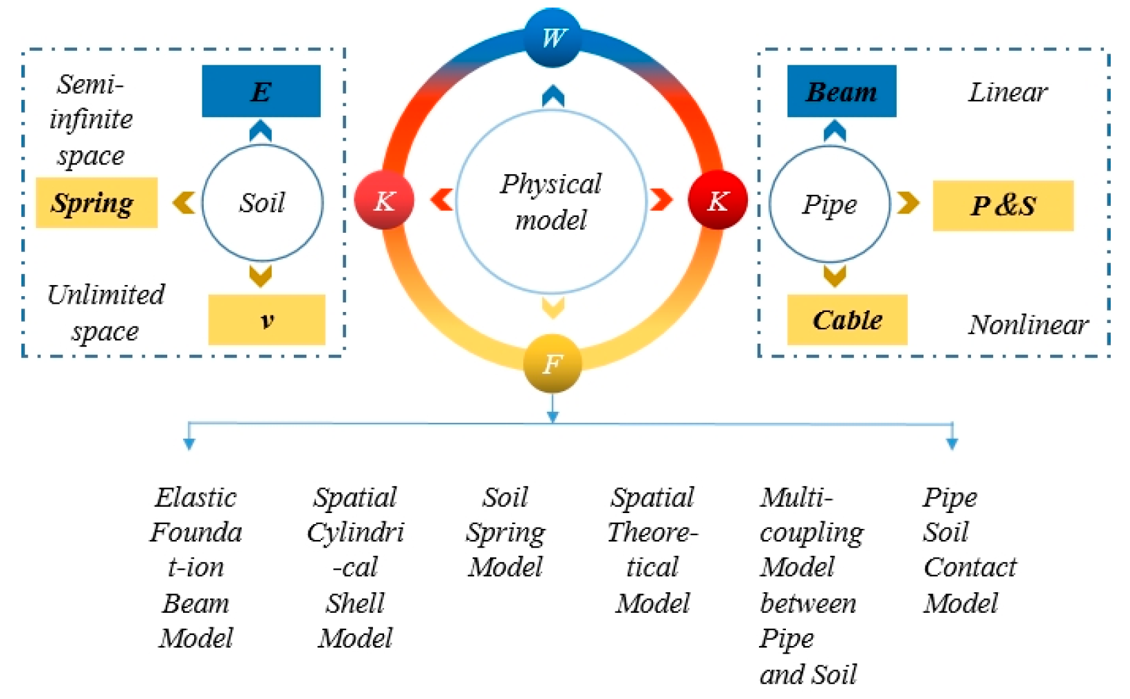
This paper systematically analyzes the coupling effects of water, heat, and force during the freezing process of soil. When comprehensively considering the seasonal variations in atmospheric temperature, the oil temperature inside the pipe, and the uneven heat transfer of the soil around the pipeline, based on the assumptions of the permafrost theory and the multi-field coupling theory, we establish the equations of the moisture field, temperature field, and stress field around the pipeline. Additionally, the partial differential equation of the interaction between pipelines and soil was derived. The research theory on pipe–soil interaction is shown in Figure 1.

2.1. Analysis of Permafrost Temperature Field

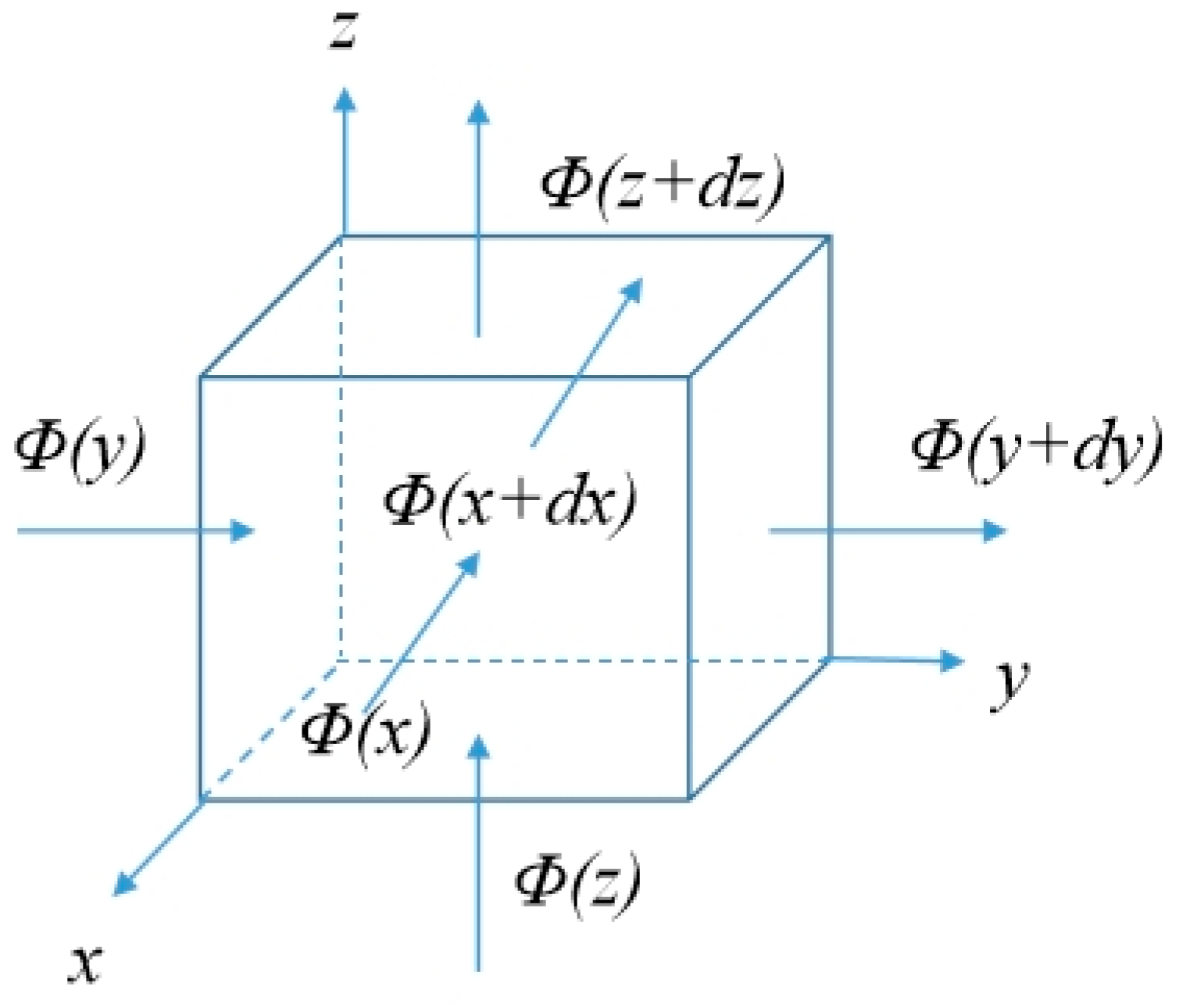
Based on the law of conservation of energy, Fourier’s law of heat conduction, and the theory of permafrost mechanics, the heat conduction equation in permafrost areas is constructed [2,26], as shown in Figure 2.

The microelement volume computing unit is selected, the partial differential equation based on Fourier’s law is established, and heat is conducted with three plane normals:

$$\left\{\begin{array}{c}{d\Phi }_{x+dx}=-(\lambda +{\displaystyle \frac{\partial \lambda }{\partial x}}dx){\displaystyle \frac{\partial }{\partial x}}(T+{\displaystyle \frac{\partial T}{\partial x}}dx)dydzdt\\ {d\Phi }_{y+dy}=-(\lambda +{\displaystyle \frac{\partial \lambda }{\partial y}}dy){\displaystyle \frac{\partial }{\partial y}}(T+{\displaystyle \frac{\partial T}{\partial y}}dy)dxdzdt\\ {d\Phi }_{z+dz}=-(\lambda +{\displaystyle \frac{\partial \lambda }{\partial z}}dz){\displaystyle \frac{\partial }{\partial z}}(T+{\displaystyle \frac{\partial T}{\partial z}}dz)dydxdt\end{array}\right.$$

(1)

Disregarding the second-order minutiae, the heat difference within the cell is:

$$\mathsf{\Delta }\Phi ={\displaystyle \frac{\partial }{\partial x}}(\lambda {\displaystyle \frac{\partial T}{\partial x}})+{\displaystyle \frac{\partial }{\partial y}}(\lambda {\displaystyle \frac{\partial T}{\partial y}})+{\displaystyle \frac{\partial }{\partial z}}(\lambda {\displaystyle \frac{\partial T}{\partial z}})$$

(2)

Free water becomes ice due to the exothermic reduction in temperature during freezing, and the heat released is recorded as the heat of phase change, which is regarded as the source term in permafrost. According to the basic theory of heat transfer and permafrost mechanics [27], the heat transfer Equation (3), which considers the latent heat of phase change, is established.

$$\rho C\left(\theta \right){\displaystyle \frac{\partial T}{\partial t}}+L\cdot {\rho }_i{\displaystyle \frac{\partial {\theta }_I}{\partial t}}=div(\lambda gradT)$$

(3)

where ρ is the density of the soil; C is the heat capacity; T is the temperature; t is the time; λ is the thermal conductivity; L is the latent heat of phase change—generally, 334.56 kJ/kg; ρ_i is the density of ice.

2.2. Analysis of Permafrost Moisture Field

Based on Darcy’s law, this paper selects the Richards equation considering phase transition and the effect of gravity as the master differential equation and establishes the water field equation as:

$${\displaystyle \frac{\partial {\theta }_u}{\partial t}}+{\displaystyle \frac{{\rho }_I}{{\rho }_w}}{\displaystyle \frac{\partial {\theta }_I}{\partial t}}=\nabla [K({\theta }_u)\nabla {\theta }_u+f({\theta }_u)]$$

(4)

where θ_u is the volumetric unfrozen water content; f is the soil permeability coefficient.

The diffusivity of water in permafrost can be calculated from Equation (4) as:

$$K({\theta }_{\mathfrak{u}})\cdot c({\theta }_{\mathfrak{u}})=f({\theta }_{\mathfrak{u}})\cdot I$$

(5)

where f(θ_u) is the permeability of the soil (m/s); c(θ_u) is the specific water capacity (1/m). I is the impedance factor, calculated as:

$$I={10}^{-10{\theta }_i}$$

(6)

f(θ_u) and c(θ_u) are calculated by the following formula:

$$\begin{array}{l}f\left({\theta }_u\right)=f_s\cdot S^l{\left(1-{\left(1-S^{1/m}\right)}^m\right)}^2\\ c({\theta }_u)=a_{0}m/(1-m)\cdot S^{1/m}{\left(1-S^{1/m}\right)}^m\end{array}$$

(7)

where a₀, m, and l are intrinsic parameters that vary with soil quality; f_s is the coefficient of permeability of saturated soil.

In order to realize the coupling between the moisture field and the temperature field, we choose the solid–liquid ratio B_i as the coupling term, which is calculated as follows:

$$B_i={\displaystyle \frac{{\theta }_i}{{\theta }_i}}\left\{\begin{array}{l}1.1{({\displaystyle \frac{T}{T_j}})}^B-1\hspace{1em}T<T_j\\ \hspace{1em}\hspace{1em}0\hspace{1em}\hspace{1em}\hspace{1em}T\ge T_j\end{array}\right.$$

(8)

The relative saturation S of the frozen soil is designed to replace θ_u for the hydrothermal coupling solution.

$$S({\theta }_s-{\theta }_v)+{\theta }_v={\theta }_u$$

(9)

where θ_s is the saturated moisture content and θ_v is the residual moisture content.

2.3. Analysis of Permafrost Stress Field

2.3.1. Effect of Pipeline Defects on the Stress Field

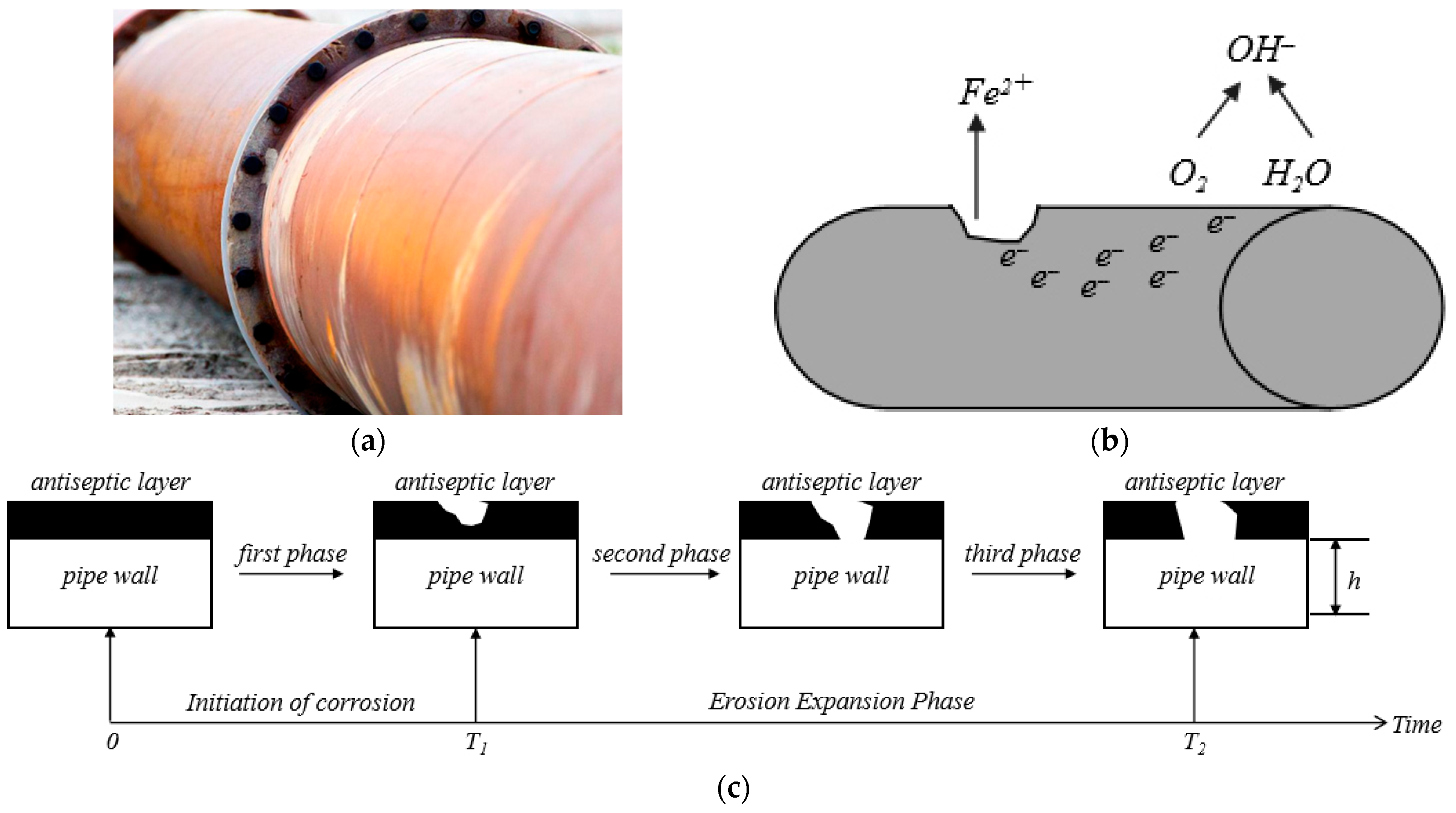
Pipeline defects include material defects, processing damage, corrosion defects, external damage, and other conditions, as shown in Figure 3. The probabilities of pipeline failure statistics in recent years are shown in

Table 1. Statistics of pipeline failure probability.

Reasons for Failure	CHINA	USA	USSR	UK
material defect	12.4	16.9	17.1	25.6
corrosion defect	43.6	35.4	41.0	30.2
process damage	25.3	29.8	15.8	12.8
sabotage by external forces	18.7	17.9	26.1	31.4

.

As can be seen from Table 1, most of the pipeline defects are due to corrosion. The combination of external forces and corrosion will lead to dents and ruptures in the pipeline, which will seriously affect the service life of the pipeline [28].

The minimum remaining wall thickness for pipe corrosion can be calculated by the following equation:

$$P_c={\displaystyle \frac{P_L{D}^2}{{\left(D+2t\right)}^2-D^2}}$$

(10)

where P_L is the internal pressure of the pipe, MPa; t is the wall thickness of the defective pipe, mm; Pc is the axial load, MPa; D is the outer diameter of the pipe, mm.

2.3.2. Stress Field Governing Equations

Under the action of the freeze–thaw cycle, the soil body is subjected to the combined effects of gravity, temperature, water pressure, and freezing and expansion forces, which leads to the deformation of the pipeline. In order to analyze the stresses generated by the soil body in the process of freezing and expansion, the soil body is assumed to be an elastomer, and the differential operator is introduced to construct the stress field equations [29]:

$$\left\{\sigma \right\}=\left[E\right]\left(\left\{\epsilon \right\}-\left\{{\epsilon }_{\nu }\right\}\right)$$

(11)

Strain resulting from moisture phase change and migration:

$${\epsilon }_{\nu }=0.09({\theta }_0+\mathsf{\Delta }\theta -{\theta }_u)+\mathsf{\Delta }\theta +({\theta }_0-n)$$

(12)

For pipes containing defects, the strain value on the pipe surface is the sum of the film strain as well as the bending strain. Since the value of the film strain in the annular direction is much smaller than the bending strain, it can be neglected, and the value of the bending strain can be calculated by the following formula:

$${\epsilon }_1={\displaystyle \frac{t}{2}}({\displaystyle \frac{1}{D_0}}-{\displaystyle \frac{1}{D_1}}),\hspace{1em}{\epsilon }_2=-{\displaystyle \frac{t}{2}}{\displaystyle \frac{1}{D_2}}$$

(13)

where ε₁ is the circumferential bending strain, ε₂ is the axial bending strain, D₀ is the outer diameter of the pipe, and D₁ is the circumferential radius of curvature of the pipe after corrosion. D₂ is the axial radius of curvature of the pipe after corrosion.

The soil strain equations considering transient strain, moisture phase change, and migration in permafrost strain calculations are as follows:

$$\epsilon ={\epsilon }_1+{\epsilon }_2+{\epsilon }_{\nu }$$

(14)

3. Numerical Simulation of Three-Field Coupling

According to the investigation data of the China–Russia pipeline, the selected pipeline material is X80M (produced in China, compliant with standard GB/T 9711-2017) grade steel, with a pipe diameter of 1219 mm. Wall thickness: 25.5 mm, design pressure: 8 Mpa, local pressure: 10 Mpa, yield strength: 530 Mpa, and tensile strength: 625 Mpa. Assuming that the soil in the computational domain is isotropic, without considering the influence of groundwater recharge and flow as well as water recharge and infiltration at other boundaries, the freeze–thaw process of the soil conforms to Darcy’s law. According to Equation (10), the middle part of the pipeline was modeled to simulate the defective pipeline. To efficiently solve the pipe–soil coupling problem, the established numerical model (as shown in Figure 4a) made full use of the circumferential symmetry of the physical process. This model typically adopts a two-dimensional axisymmetric simplified assumption, that is, it assumes that the distribution of the temperature field, moisture field, and stress field around the pipeline is rotationally symmetrical about the central axis of the pipeline. This symmetry-based model simplification ensures that the key physical mechanisms are accurately captured while significantly reducing the computational complexity. By adopting a differentiated grid strategy, the pipeline structure is generated into a hexahedral dominant grid through the scanning method and locally densified. The soil is divided into tetrahedral grid cells. The total number of model grids is 325,414, and the grid division is shown in Figure 4b. Based on the on-site soil data, the unstable sample soil was selected as the simulated soil mass. The basic parameters of the soil and pipelines are shown in

Table 2. Basic Properties of Soil.

Soil	Density (kg·m−3)	Moisture	Thermal Conductivity [(J·(m·h·K)−1]	Specific Heat [J·(kg·K)−1]	Porosity Ratio
loess	1970	0.3	6552	982	0.63

and

Table 3. Basic Properties of Pipes.

Title	Material	Density (kg·m−3)	Modulus of Elasticity (GPa)	Poisson’s Ratio
pipe	X80	7850	200	0.3

.

3.1. Multi-Field Coupling Boundary Conditions

3.1.1. Temperature Field Boundary Conditions

Since the atmospheric temperature changes continuously with time, the upper boundary of the study area is selected as the boundary condition of convective heat exchange between the atmosphere and the soil surface with a heat exchange coefficient of 18 W·(m² °C)⁻¹. The upper boundary condition can be expressed as:

$$T=T_0+\alpha t+\beta \sin ({\displaystyle \frac{2\pi t}{8760}}+\phi )$$

(15)

where T₀ is the annual mean atmospheric temperature; α is the annual mean surface temperature warming rate; β is the heat exchange coefficient; and φ is the phase difference.

The left and right boundaries of the calculation domain are set as adiabatic boundaries, and the boundary heat flux is 0; the soil bottom temperature is set to −2 °C according to the survey data, and the oil temperature inside the pipeline is set to 20 °C.

3.1.2. Moisture and Stress Field Boundary Conditions

The moisture field is set according to the actual physical parameters of the soil, and the moisture content of the soil is 0.3. The moisture content of the piping material is 0. All boundaries of the computational domain do not exchange moisture with the atmosphere and are set as zero-flux boundaries.

The bottom of the structural computational domain is a fixed boundary with left and right constraints on x-direction displacements.

$$\begin{array}{l}\mid x\mid =a,\hspace{1em}{\tau }_{xy}=0;\hspace{1em}y=-b,\hspace{1em}{\sigma }_x=0\\ \mid x\mid =a,\hspace{1em}\mu =0;\hspace{1em}y=-b,\hspace{1em}\nu =0\end{array}$$

(16)

3.2. Numerical Model Validation

The partial differential equations of Equations (3), (4), and (14) are established and inputted into the simulation software (COMSOL Multiphysics^® 6.0, developed by COMSOL Inc., Burlington, MA, USA) to obtain the two-dimensional cross-section results of the pipe–soil model to verify the accuracy of the numerical model. Analysis of the influence of parameters on the mechanical properties of pipes.

3.2.1. Temperature

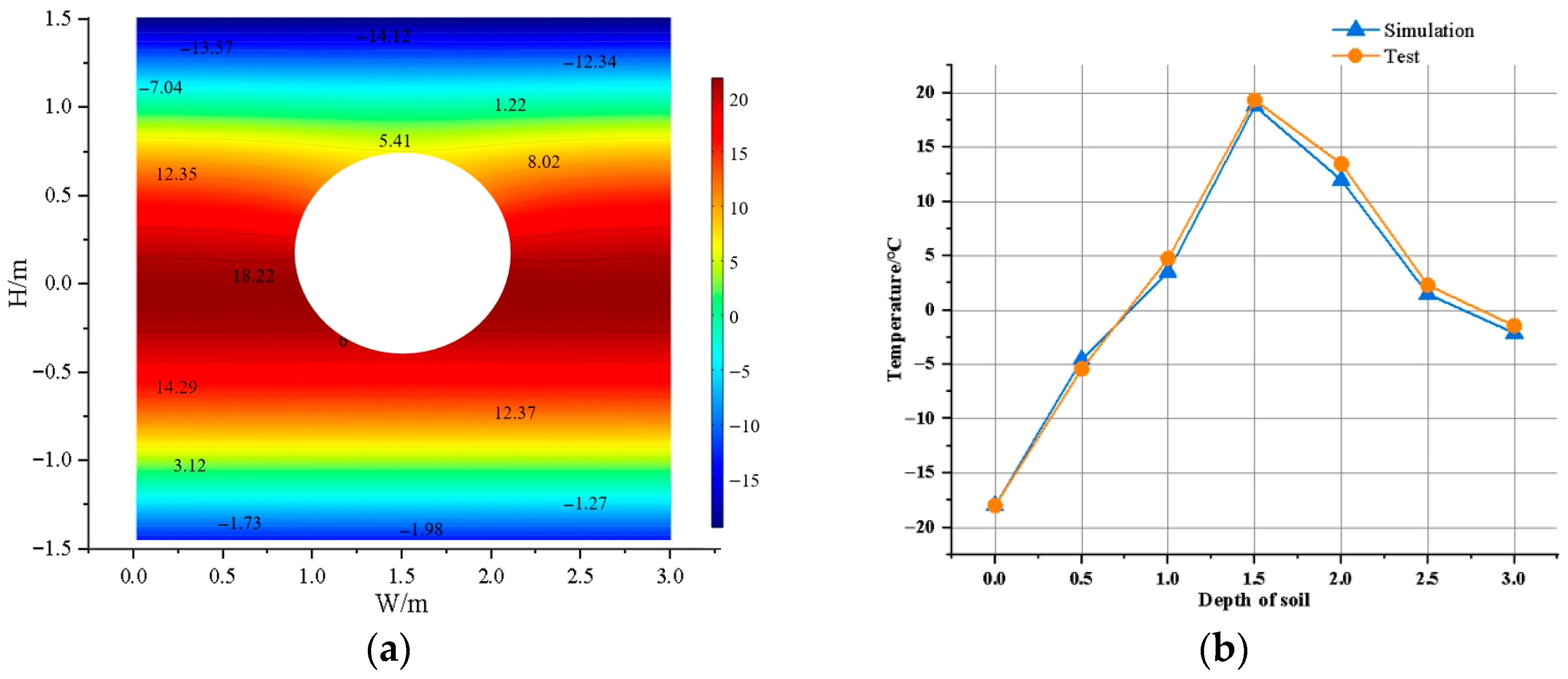
Figure 5a shows the temperature conditions simulated in January when the soil moisture content is 30% and the pipeline burial depth is 1.2 m. The temperature curve along the depth of the soil at a distance of 1 m from the central axis of the pipeline was selected and compared with the on-site monitoring temperature. As can be seen from Figure 5b, the numerical simulation temperature is consistent with the on-site monitoring data, with a maximum temperature error of 1.49 °C, verifying the accuracy of the temperature field simulation.

Based on the relevant grid division rules of the tube-and-soil model in the literature [30], this paper ensures simulation accuracy while reducing computational load. The grid sensitivity analysis is conducted using grid cell numbers of 325,414, 264,789, and 473,245, respectively. The optimal grid quality is selected by comparing the errors between the temperature field simulation results and the test results. The comparison table is shown in

Table 4. Grid sensitivity analysis.

Number of Grid Cells	Error Analysis
325,414	6.76%
214,789	9.43%
573,245	4.89%

. It can be seen from the table that an increase in the number of grids can improve accuracy, but the computational load will increase exponentially. Therefore, when the number of elements is 325,414, it can meet the simulation accuracy requirements.

3.2.2. Soil Water Content

To further verify the accuracy of the theoretical model, ignoring the influence of pipeline oil temperature, the soil moisture content was simulated at a horizontal distance of 1 m from the pipeline under 20 freeze–thaw cycles. The maximum deviation of water content between the measured data and the simulated data in Figure 6 is 2%, which verifies the accuracy of the water field simulation.

3.3. Analysis of the Influence of Different Parameters on the Mechanical Properties of Pipelines

In practical engineering applications, there are more factors affecting the mechanical properties of pipelines, and the mapping mechanism of initial water content, pipe burial depth (top of pipe), pipe diameter, and wall thickness on the mechanical properties of pipelines is investigated through three-field coupled simulation of the pipelines. The results are analyzed and the dataset is constructed. The value ranges of the four parameters are shown in

Table 5. Parameter value range.

Parameter Name	Range of Values
initial water content	0.2~0.3
depth of burial (m)	1.2~1.5
pipe diameter (mm)	1011~1417
wall thickness (mm)	17.5~37.5

.

3.3.1. Effect of Initial Moisture Content

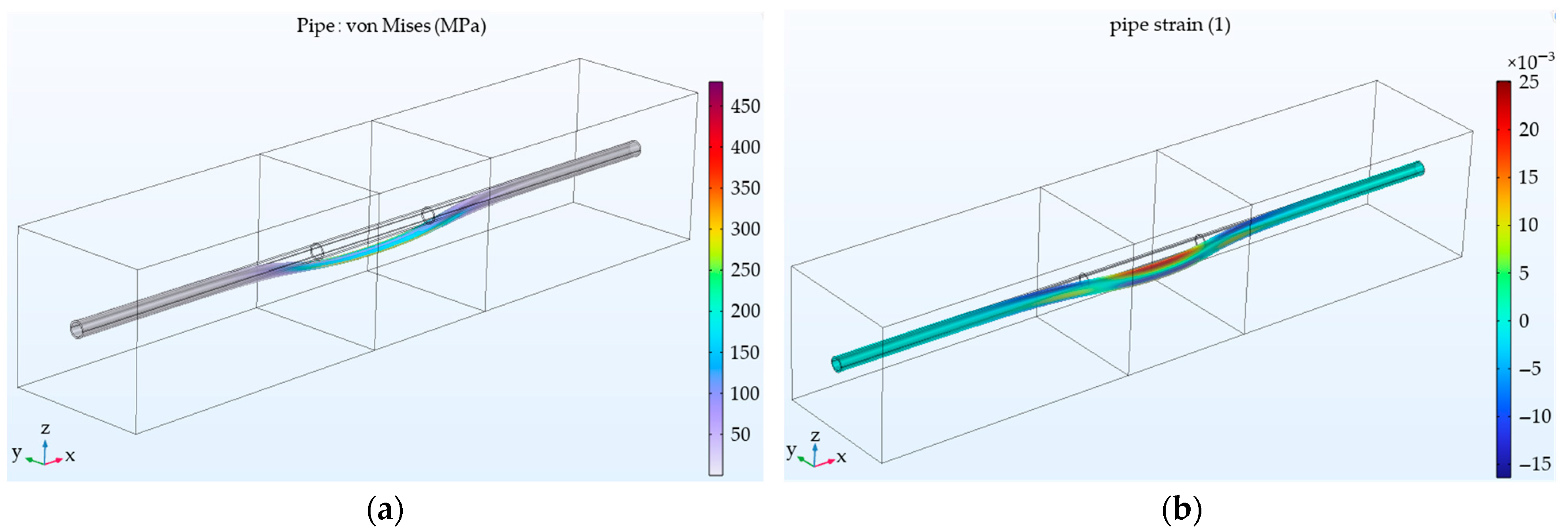
The pipe is buried at a depth of 1.2 m, with a diameter of 1219 mm and a wall thickness of 25.5 mm. Without considering the internal pressure of the pipe, the equivalent stresses and strains of the pipe are shown in Figure 5 when comparing different water contents.

As shown in Figure 7a,b, the overall stress and strain distribution cloud map of the pipeline presents a high degree of circumferential symmetry, which is in line with the expected mechanism of frost heave force. However, there is symmetry breaking in some local areas (especially near the defect), showing a distinct strain concentration phenomenon, which confirms the significant disturbance of the defect on the mechanical response. Figure 8 and

Table 6. Stress–strain condition of pipeline under different initial moisture content.

Initial Moisture Content of the Soil	Pipe Equivalent Force (MPa)	Pipeline Isotropic Strain
0.3	327.62	0.00164
0.25	297.86	0.00149
0.2	262.1	0.00135

further reveal that after 20 freeze–thaw cycles, when the initial moisture content of the soil is 0.3, the effect force of pipelines and others reaches 327.62 MPa, which increases by 9.10% and 20.1%, respectively, compared with the other two groups. The equivalent strain increase also reached 9.15% and 17.7%, respectively. This indicates that an increase in water content intensifies the frost heaving effect—the pore water phase turns into ice, causing soil compaction and enhancing the interaction between soil particles, thereby significantly increasing the equivalent stress of the pipeline.

3.3.2. Effect of Burial Depth

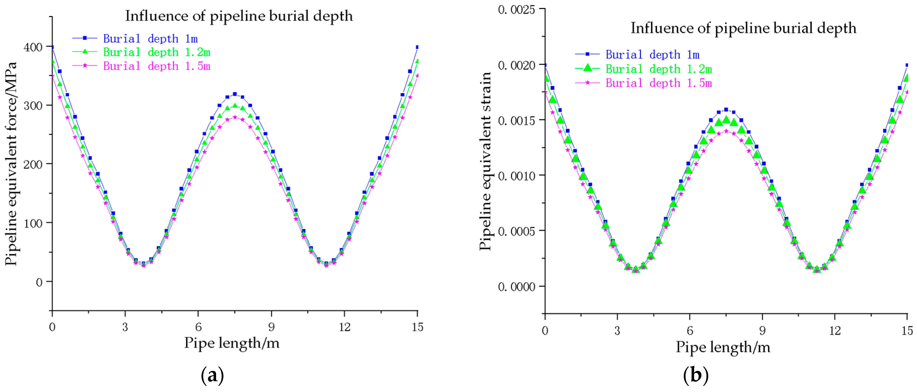
The initial moisture content of the soil is 0.25, the diameter of the pipe is 1219 mm, the wall thickness is 25.5 mm, and the equivalent stresses and strains of the pipe under the action of 20 freeze–thaw cycles of data collection are shown in Figure 9, comparing the different depths of burial of the pipe without considering the internal pressure of the pipe.

From Figure 9 and

Table 7. Stress–strain condition of pipeline under different initial water content.

Pipe Burial Depth (m)	Pipe Equivalent Force (MPa)	Pipeline Isotropic Strain
1.0	315.44	0.00157
1.2	297.86	0.00149
1.5	285.44	0.00143

, it can be seen that after the frost expansion of the soil, the equivalent stress and strain of the pipeline decreased by 1.51% and 4.03%, respectively, when comparing the burial depth of the pipeline of 1.5 m with that of the pipeline of 1.2 m, and decreased by 5.23% and 5.10%, respectively, when comparing the burial depth of the pipeline of 1.2 m with that of the pipeline of 1 m. It can be concluded from the results that with the increase in burial depth, the equivalent stress and strain of the pipeline will be reduced, and the degree of stress and strain reduction gradually decreases with the increase in burial depth.

3.3.3. Pipe Diameter Impact

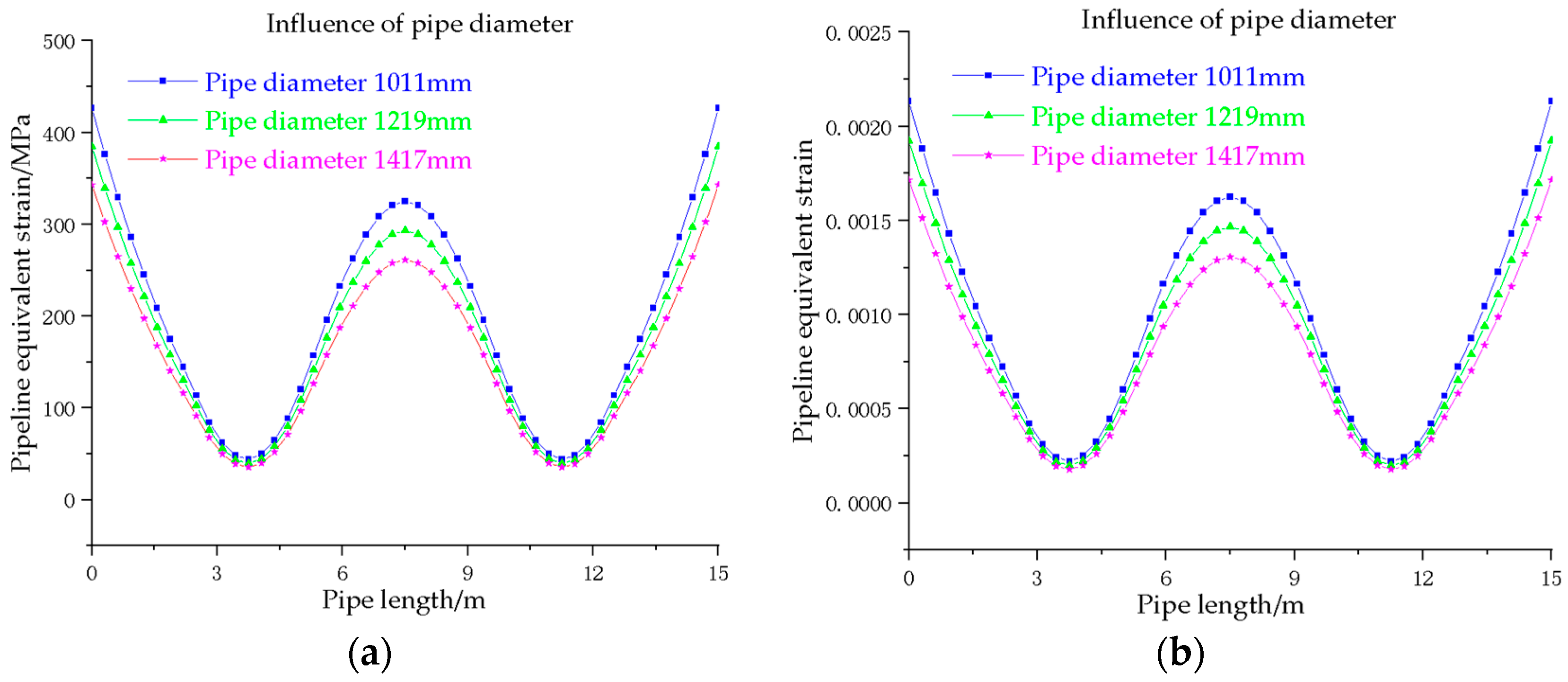
The initial moisture content of the soil is 0.25, the burial depth of the pipe is 1.2 m, and the wall thickness is 25.5 mm. Without considering the internal pressure of the pipe, comparing different pipe diameters, the equivalent stresses and strains of the pipe under the action of 20 freeze–thaw cycles of data collection are shown in Figure 10.

From Figure 10 and

Table 8. Stress–strain conditions of pipes with different pipe diameters.

Pipe Diameter (mm)	Pipe Equivalent Force (MPa)	Pipeline Isotropic Strain
1011	325.13	0.00162
1219	297.86	0.00149
1417	261.38	0.00133

, it can be seen that the equivalent force and equivalent strain of the pipe decreased by 8.39% and 8.02%, respectively, when comparing the 1219 mm pipe diameter with the 1011 mm pipe diameter, and by 12.2% and 10.74%, respectively, when comparing the 1417 mm pipe diameter with the 1219 mm pipe diameter, after frost damage occurred in the soil. It can be seen that the pipe diameter can be increased to avoid freezing damage to the pipe under the consideration of cost conditions.

3.3.4. Pipe Wall Thicknesses Impact

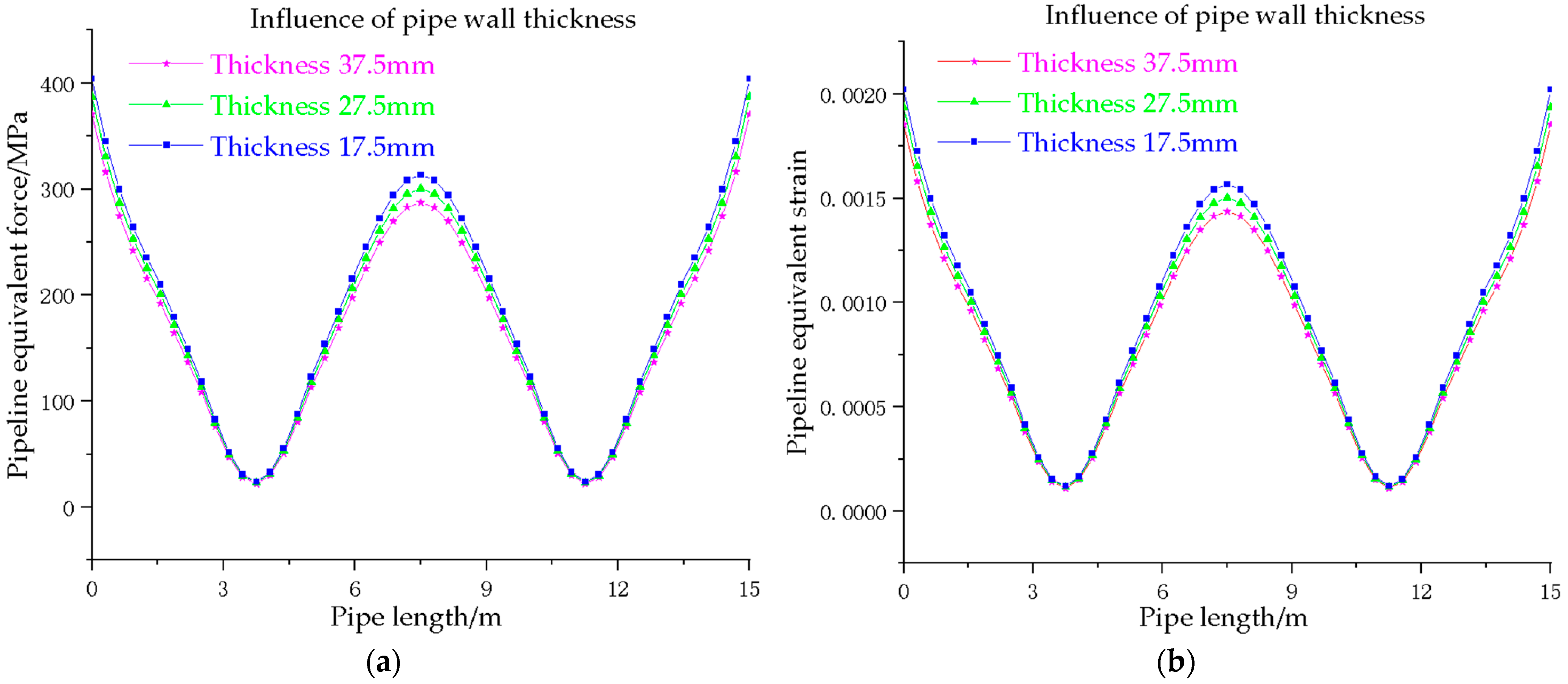
The initial water content of the soil is 0.25, the burial depth of the pipe is 1.2 m, and the diameter of the pipe is 1219 mm. Without considering the internal pressure of the pipe, comparing different pipe wall thicknesses, the equivalent stresses and strains of the pipe under the action of 20 freeze–thaw cycles of data collection are shown in Figure 11.

From Figure 11 and

Table 9. Stress–strain conditions of pipes with different wall thicknesses.

Wall Thickness (mm)	Pipe Equivalent Force (MPa)	Pipeline Isotropic Strain
17.5	313.62	0.00157
27.5	297.86	0.00149
37.5	287.48	0.00142

, it can be seen that the equivalent force and equivalent strain of the pipe decreases by 3.48% and 4.70%, respectively, when wall thickness of 37.5 mm is compared with wall thickness of 27.5 mm and by 5.03% and 5.11%, respectively, when wall thickness of 27.5 mm is compared with wall thickness of 17.5 mm after freezing and expansion of the soil occurs. The results show that the pipe equivalent stress and strain decreases with the gradual increase in the pipe wall thickness.

Looking at Figure 9a,b, Figure 10a,b, and Figure 11a,b, the comparison diagrams of equivalent stress and equivalent strain of pipes under different initial water content/burial depth/pipe diameter/wall thickness conditions further confirm that despite changes in external parameters, the basic mode of pipe deformation caused by frost heave (such as bending) and its potential symmetry framework remain consistent. The parameter variation mainly affects the strain magnitude rather than the fundamental deformation symmetry morphology.

4. Analysis of Pipeline Safety Under Freeze–Thaw Cycles

4.1. Pipe Failure Modeling

The traditional pipeline failure model is established based on the stress-based analysis method; after the freeze–thaw cycle, the pipeline will have a local large deformation under the action of the soil, which will lead to the excessive safety margin of the pipeline and the high cost of pipeline construction. Therefore, this paper adopts the strain-based analysis method.

Tensile fracture and compressive buckling of the pipe will occur under the action of pipe soil, so it is necessary to check the ultimate tensile strain and ultimate compressive strain of the pipe and establish the pipe failure model based on the strain design criterion.

$$T=\left[\epsilon \right]-\epsilon$$

(17)

where ε is the maximum tensile strain of the pipe; [ε] is the allowable strain of the pipe. When the maximum tensile strain or compressive strain of the pipe is greater than the allowable strain of the pipe, the pipe will be damaged. Therefore, the pipe failure function can be defined as:

$$T=f(\left[\epsilon \right],\epsilon )=\left[\epsilon \right]-\epsilon$$

(18)

The permissible strain for pipelines in permafrost zones according to the Technical Standards for Strain-Based Design of Oil and Gas Pipeline Line Projects:

$$S·\left[\epsilon \right]={\epsilon }^{cri}$$

(19)

where [ε] is the permissible strain of the pipe, ε^cri is the ultimate tensile strain, and S is the safety factor. In this paper, the ultimate tensile strain value of the pipe is 2%, and the permissible strain is calculated to be 1.6%.

4.2. Constructing Response Surface Functions Based on Pipe Strain

The response surface analysis method can establish an explicit approximate functional relationship between input parameters and output responses, which is convenient for subsequent analysis. It has strong visualization ability and it is easy to understand the interaction between parameters. It is particularly suitable for the nonlinear and multi-parameter problem of permafrost–pipeline interaction involved in this study.

Compared with the sensitivity analysis method, the response surface method has the advantages of less calculation time consumption, avoiding repetitive experiments, and it can quantify the second-order interaction terms between parameters, while the sensitivity analysis method can only identify the main effect.

4.2.1. Design Sample Point Determination

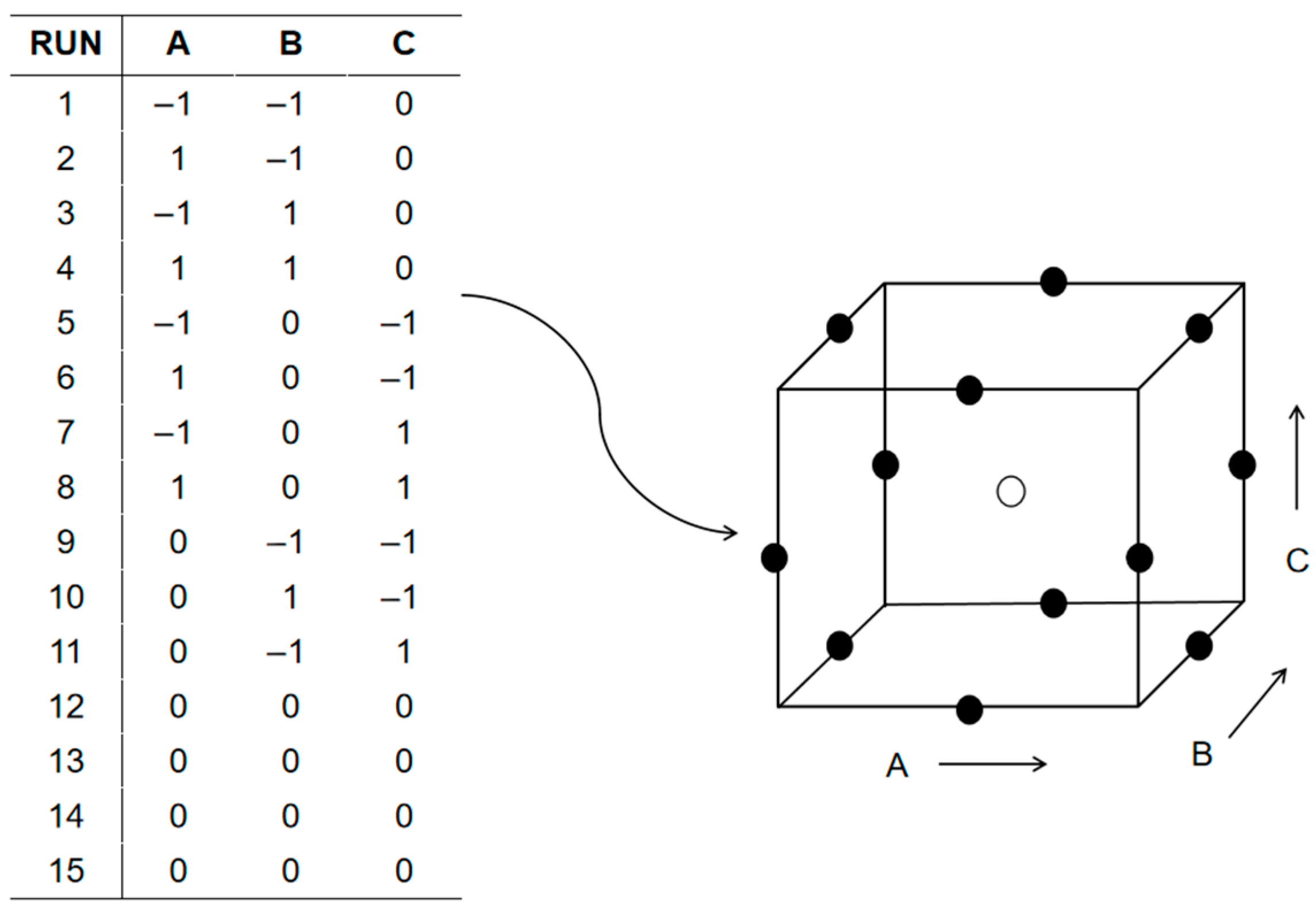
In this paper, a Box–Behnken design is used, which analyzes the nonlinear relationship between the underlying variables and the response outcomes without the need for multiple consecutive experiments and allows for the prediction of all main effects, the two-way interaction effect, and the squared term of each factor. The design is created by taking three probability level points for each random variable and randomly arranging and combining sample points consisting of edge centers and centroids according to the rules given in the design, as shown in Figure 12.

According to the simulation results in Section 3, it is known that the three factors that have a greater influence on the equivalent strain of the pipeline are the depth of burial, pipe diameter, and wall thickness, so in the analysis of pipeline safety, the depth of burial h, the pipe diameter l, and the wall thickness t are selected for analysis.

The probability levels of the three variables are expressed as −1, 0, and 1, respectively. They represent the low level, medium level, and high level, respectively. The experimental design matrix is obtained through combined design, as shown in

Table 10. Test design matrix.

Sample Point Number	h	l	t
1	−1	−1	0
2	1	−1	0
3	−1	1	0
4	1	1	0
5	−1	0	−1
6	1	0	−1
7	−1	0	1
8	1	0	1
9	0	−1	−1
10	0	1	−1
11	0	−1	1

.

The probability level point x_a of the random distribution is:

$${\displaystyle \underset{-\infty }{\overset{x_a}{\int }}P(x)dx=A_n},n=1,2,3$$

(20)

Based on the experimental design matrix shown in Table 10, all sample point groups were obtained by the equation, as shown in

Table 11. Sample points and response values by Box–Behnken method.

Sample Point Number	h (m)	l (m)	t (m)	Maximum Tensile Strain ε (%)
1	1.00	1.417	0.0275	0.001512
2	1.50	1.214	0.0375	0.001513
3	1.25	1.417	0.0175	0.001482
4	1.50	1.417	0.0275	0.001494
5	1.25	1.214	0.0275	0.001530
6	1.25	1.011	0.0175	0.001606
7	1.00	1.011	0.0275	0.001606
8	1.25	1.417	0.0375	0.001465
9	1.00	1.214	0.0375	0.001546
10	1.25	1.214	0.0275	0.001530
11	1.25	1.011	0.0375	0.001529
12	1.50	1.011	0.0275	0.001589
13	1.00	1.214	0.0175	0.001578

. The sample points in the table were substituted into the simulation software (COMSOL Multiphysics^® 6.0, developed by COMSOL Inc., Burlington, MA, USA) for the numerical solution to obtain the maximum tensile strain.

4.2.2. Response Surface Function Construction

According to the response surface function construction theory, taking the burial depth h, pipe diameter l, and wall thickness t as the basic variables, and based on the multivariate binomial mathematical model, the influence of the three basic variables on the maximum tensile strain value of the pipeline is analyzed by the least-squares fitting method, and the response surface function is constructed as:

$$\begin{array}{l}\epsilon =0.002471-1.003\times {10}^{-3}h-6.9\times {10}^{-5}l-5.53\times {10}^{-3}t+4.2\times {10}^{-4}{h}^2\\ -1.52\times {10}^{-4}{l}^2-3.75\times {10}^{-2}{t}^2-3\times {10}^{-3}ht+7.39\times {10}^{-3}lt\end{array}$$

(21)

The constructed response surface function contains not only primary and secondary terms but also quadratic cross-terms; thus, it can greatly improve the analysis of pipeline safety under freeze–thaw cycles.

In order to verify the reliability of the Box–Behnken design [31], the results of the response surface function fitting calculated for each sample point in Table 10 are compared with the maximum tensile strains obtained from the simulation, as shown in

Table 12. The eigenvalue of RSM model.

Characteristic Parameters	R-Squared	Adj R-Squared	Pred R-Squared	Adeq Precision
Numerical value	95.86%	90.40%	88.34%	20.315

.

It can be seen from

Table 13. Comparison table of fitting situation.

Sample Point Number	Maximum Tensile Strain for RSM Fitting (%)	Maximum Tensile Strain Calculated by Simulation (%)	Relative Error (%)
1	0.001512	0.001512	0.00
2	0.001513	0.001484	1.94
3	0.001482	0.001452	2.01
4	0.001494	0.001455	2.59
5	0.001530	0.001492	2.47
6	0.001606	0.001576	1.85
7	0.001606	0.001596	0.62
8	0.001465	0.001435	2.03
9	0.001546	0.001507	2.50
10	0.001530	0.001492	2.47
11	0.001529	0.001510	1.25
12	0.001589	0.001569	1.26
13	0.001578	0.001568	0.64

that the maximum error between the fitting result of the response surface function and the simulation result is 2.59%, and the fitting effect is good.

5. Experimental Studies

In order to verify the constructed response surface function, this paper is based on Bockingham’s π theorem and carries out the scaled-down test to investigate the pipe strain under the action of freeze–thaw cycles. The control variable method is adopted, and the pipe burial depth, initial water content, and the number of freeze–thaw cycles are selected as variables.

5.1. Similarity Criteria and Scaling Design

According to the similarity theorem, equilibrium equations, geometric equations, and linear elasticity physics equations, the similarity criterion number of the pipe–soil interaction model is established with π. In this paper, a 20:1 scale-down model is established, with the geometric similarity ratio of C_l = 20, and in order to make the experimental model consistent with the original model, it is necessary to keep the similarity criterion number of π unchanged, and the similarity ratio number of the temperature change cycle is C_t = 400. According to the calculation of a year of 365 days, the scale-down model is established. According to the calculation of 365 days a year, the established scaling model has a period of 22 h, and the test is set up with 11 h cooling and 11 h warming.

If the stress similarity ratio C_σ = 1 is made, then the soil material has a modulus of elasticity similarity ratio C_E = 1, a strain similarity ratio C_ε = 1, and the displacement similarity ratio is the same as the geometric similarity ratio.

$$\pi ={\displaystyle \frac{b{C}_l^2}{C_t}}$$

(22)

5.2. Test Setup

According to the scaling model, the test setup is designed as shown in the figure below, with a box size of 1000 mm × 600 mm × 600 mm, which includes a box frame structure (box wall, gimbals, and handles), with strain gauges glued to the ends and the middle part of the pipe, and the specific arrangement as shown in Figure 13.

The specific test materials and geometric parameters are shown in

Table 14. Material and geometrical parameters.

Test Group	Physical Quantity	Simulation Prototype	Test Selection
Pipe	Piping materials	X80	X80
	Pipe geometry/mm	1219 × 25	D60 × t1.0 × L1000
Soil	Soil geometry/m	L75 × W14 × H10	L1 × W0.6 × H0.6
	Soil material	Field prototype soil	Loess

below:

The test conditions are shown in

Table 15. Test conditions.

Test Group	Depth of Burial/mm	Initial Moisture Content	Pipe Diameter/mm	Wall Thickness/mm
U-1	200	20%	60	1
U-2	200	25%	60	1
U-3	200	30%	60	1
V-4	240	20%	60	1
V-5	240	25%	60	1
V-6	240	30%	60	1
W-7	300	20%	60	1
W-8	300	25%	60	1
W-9	300	30%	60	1

below:

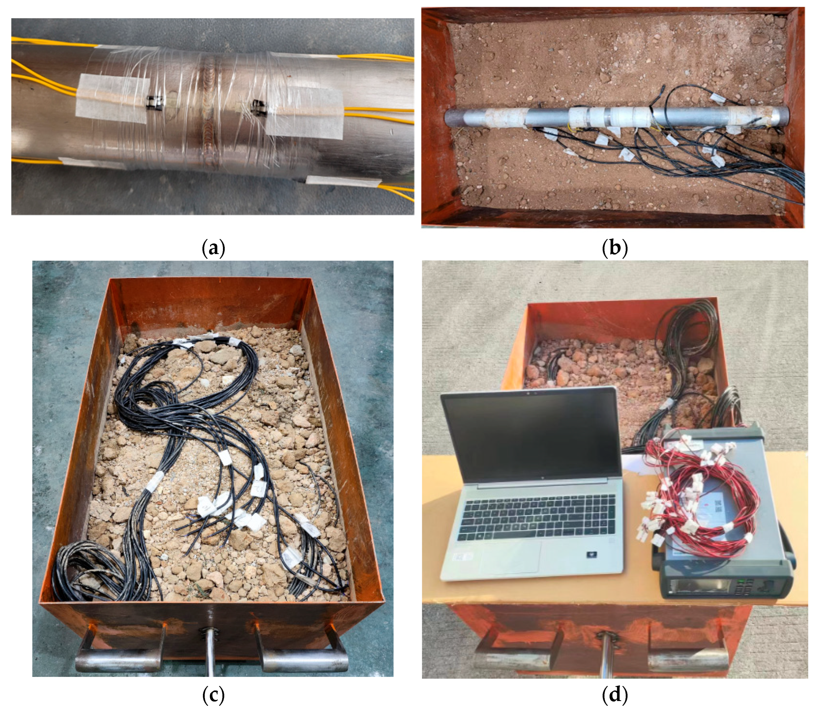
The freeze–thaw process was carried out in a freezer at −18 ± 1 °C, and the thaw–sinking process was carried out outdoors to simulate a summer environment. Data were tested after 22 h of freeze–thaw cycles, as shown in Figure 14a–d.

5.3. Analysis of Test Results

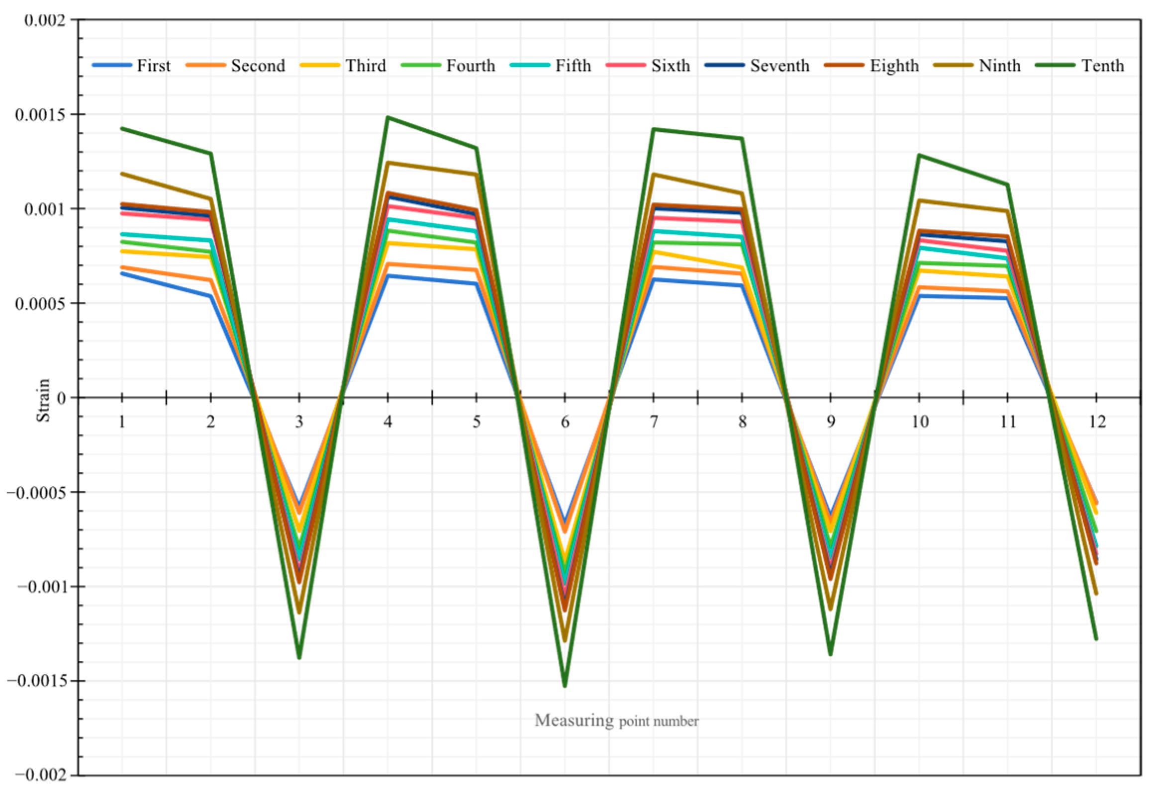
The strains at the top, bottom, and sides of the pipe were obtained from test U-1, as shown in Figure 15.

It can be seen from the figure that with the freeze–thaw cycles, tensile strain occurred at the top of the pipe and the values were all positive, while compressive strain occurred at the bottom of the pipe and the values were negative. As the number of freeze–thaw cycles increases, the strain values of the pipe also increase, and the strain values are large due to the fact that the measurement points 4–9 are located at the pipe defects, where the strength of the pipe decreases.

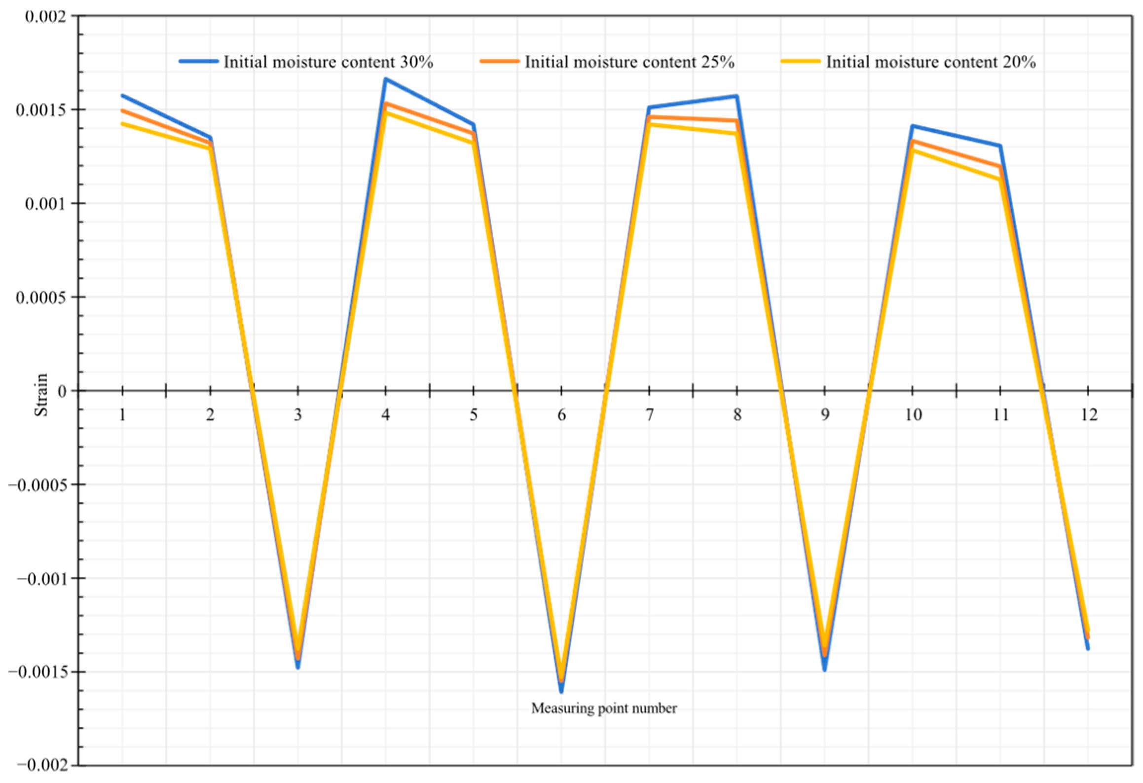
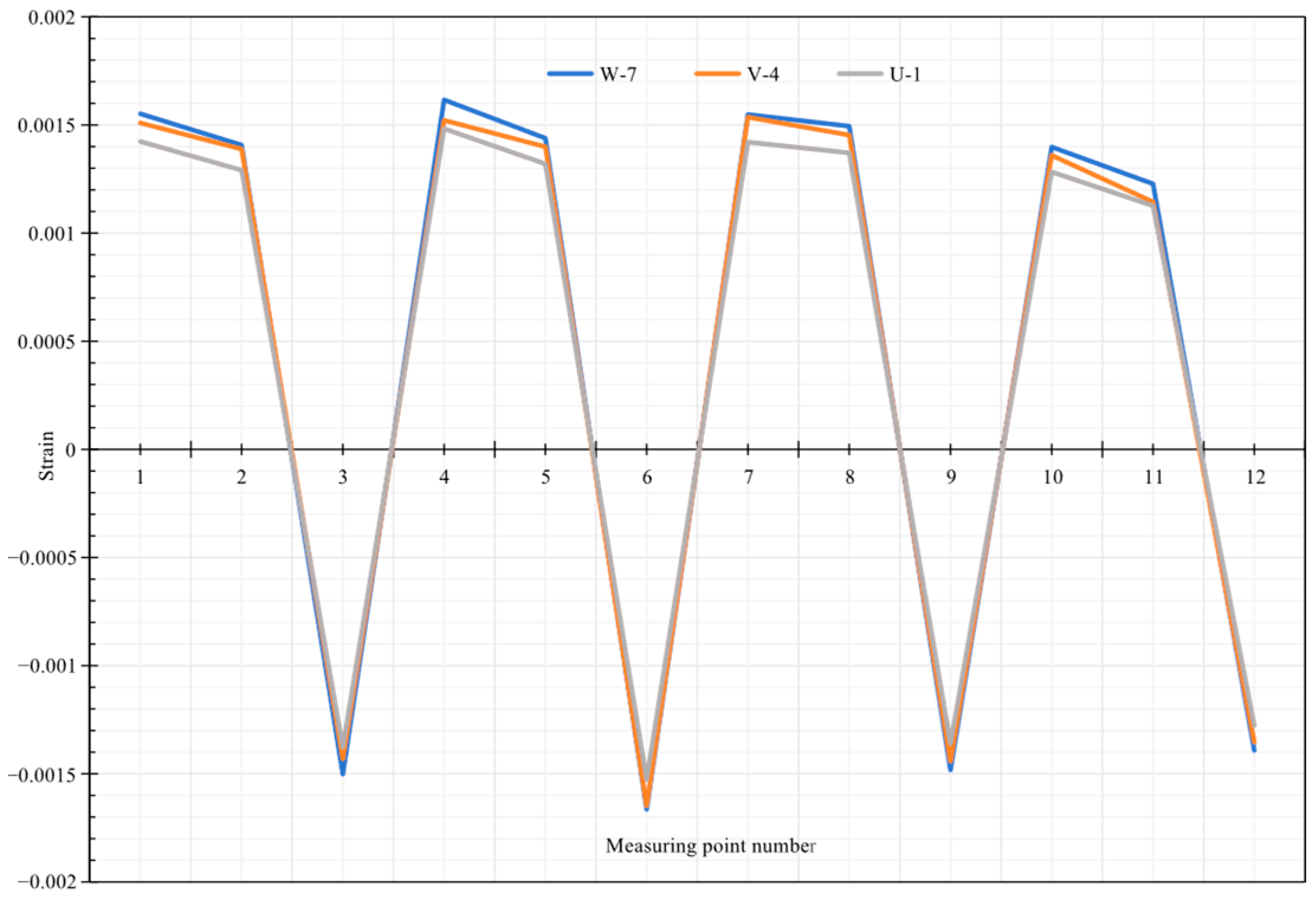
Figure 16 compares the pipe strains in U-1, U-2, and U-3, and the three curves yield that the lower the initial water content, the smaller the strain produced by the pipe, which is due to the fact that with the freeze–thaw cycling effect, the lower the initial water content, the slower the rate of change in water content, and the lower the strain produced by the pipe. The test results in W-7, V-4, and U-1 are recorded in Figure 17, and analyzing the pipe strains, it can be concluded that the deeper the pipe is buried, the larger the pipe strain is, which is consistent with the simulation law.

6. Conclusions

This study focuses on defective buried pipelines in permafrost regions. By establishing a multi-field coupling numerical model based on PDE (temperature–moisture–stress field), the strain evolution of pipelines under freeze–thaw cycles is systematically simulated. Safety analysis is conducted using Box–Behnken design, and the reliability of the model is finally verified through experiments. The constructed theoretical framework fully utilizes the circumferential symmetry principle of permafrost–pipeline interaction, and simultaneously reveals that understanding this symmetry and its breaking mechanism under defect/non-uniform conditions is the physical basis for accurately predicting pipeline deformation and evaluating the safety of pipelines with defects. Based on the research content of this paper, there are mainly the following conclusions:

• A three-field coupled PDE framework was established to resolve large-deformation challenges in pipe–soil systems. The model achieved >90% accuracy in predicting strain distribution compared to experimental data, addressing gaps in existing analytical approaches.
• Based on the multi-field coupling theory, a pipe–soil coupling simulation model is established to reveal the influence of initial water content, burial depth, pipe diameter, and wall thickness on the geometric deformation and strain of the pipe. The results show that different initial water contents have a significant effect on the pipe strain, and the maximum tensile strain of the pipe decreases with the increase in the depth of burial, and decreases with the increase in the wall thickness and pipe diameter.
• Response surface analysis revealed that water content and burial depth dominate pipeline failure risk. Optimized parameters reduced thaw–settlement failure probability by 65%, providing actionable guidelines for permafrost pipeline protection.
• The accuracy of the simulation of defective pipes was verified by designing a pipe–soil scaling model and conducting freeze–thaw cycle tests. Compared with the non-defective place, the deformation of the pipeline is obviously smaller than that of the defective place, so in the process of protecting the pipeline, it is necessary to consider the wear and corrosion of the pipeline.

References

1. Akhtar, S.; Li, B. Numerical analysis of pipeline uplift resistance in frozen clay soil considering hybrid tensile-shear yield behaviors. Int. J. Geosynth. Ground Eng. 2020, 6, 47. [Google Scholar] [CrossRef]
2. Dayarathne, R.S.; Hawlader, B.C.; Phillips, R. Centrifuge modelling of gas pipelines undergoing freeze–thaw cycles. Can. Geotech. J. 2022, 59, 485–497. [Google Scholar] [CrossRef]
3. Deng, F.; Lu, J.; Wan, X.; Liu, B.; Zhang, B.; Fu, H. Mitigating frost heave of a soil stabilized with sisal fiber exposed to freeze-thaw cycles. Geotext. Geomembr. 2025, 53, 394–404. [Google Scholar] [CrossRef]
4. Li, H.; Lai, Y.; Wang, L.; Yang, X.; Jiang, N.; Li, L.; Wang, C.; Yang, B. Review of the state of the art: Interactions between a buried pipeline and frozen soil. Cold Reg. Sci. Technol. 2019, 157, 171–186. [Google Scholar] [CrossRef]
5. Li, S.; Lai, Y.; Zhang, M.; Pei, W.; Zhang, C.; Yu, F. Centrifuge and numerical modeling of the frost heave mechanism of a cold-region canal. Acta Geotech. 2019, 14, 1113–1128. [Google Scholar] [CrossRef]
6. Ma, Q.; Fu, H.; Xiao, H.; Liu, Y.; Zhang, J.; Deng, Q. Model test study on mechanical properties of pipe under the soil freeze-thaw condition. Cold Reg. Sci. Technol. 2020, 174, 103040. [Google Scholar] [CrossRef]
7. Wang, F.; Li, G.; Ma, W.; Wu, Q.; Serban, M.; Vera, S.; Alexandr, F.; Jiang, N.; Wang, B. Pipeline–permafrost interaction monitoring system along the China–Russia crude oil pipeline. Eng. Geol. 2019, 254, 113–125. [Google Scholar] [CrossRef]
8. Everett, D.H. The thermodynamics of frost damage to porous solids. Trans. Faraday Soc. 1961, 57, 1541–1551. [Google Scholar] [CrossRef]
9. Miller, R.D. Freezing and heaving of saturated and unsaturated soils. Highw. Res. Rec. 1972, 393, 1–11. [Google Scholar]
10. Jeon, S.; Kim, Y. Numerical simulation of level ice–structure interaction using damage-based erosion model. Ocean Eng. 2021, 220, 108485. [Google Scholar] [CrossRef]
11. Chen, J.; Gao, X.; Zheng, X.; Miao, C.; Zhang, Y.; Du, Q.; Xu, Y. Simulation of soil freezing and thawing for different groundwater table depths. Vadose Zone J. 2019, 18, 1–14. [Google Scholar] [CrossRef]
12. Wei, Y.J.; Wen, Z.; Gao, Q.; Zhang, M.L.; Shi, R.; Kong, S. Numerical analysis of temperature fields around the buried gas pipeline in permafrost regions of Qinghai-Tibet Plateau. J. Glaciol. Geocryol. 2019, 41, 1078–1086. [Google Scholar]
13. Nasery, M.M.; Ağcakoca, E.; Sert, S.; Sadid, M.S.; Yaman, Z. The effect of ground improvement materials on the impact resistance and behavior of buried pipes: An experimental and numerical study. Tunn. Undergr. Space Technol. 2025, 163, 106761. [Google Scholar] [CrossRef]
14. Lei, D.; Yang, Y.; Cai, C.; Chen, Y.; Wang, S. The Modelling of Freezing Process in Saturated Soil Based on the Thermal-Hydro-Mechanical Multi-Physics Field Coupling Theory. Water 2020, 12, 2684. [Google Scholar]
15. Yin, X.; Liu, E.; Song, B.; Zhang, D. Numerical analysis of coupled liquid water, vapor, stress and heat transport in unsaturated freezing soil. Cold Reg. Sci. Technol. 2018, 155, 20–28. [Google Scholar] [CrossRef]
16. Zhang, X.; Wu, Y.; Zhai, E.; Ye, P. Coupling analysis of the heat-water dynamics and frozen depth in a seasonally frozen zone. J. Hydrol. 2021, 593, 125603. [Google Scholar] [CrossRef]
17. Li, Q.; Zhang, D.; Li, P.; Cui, K.; Jing, X. The small-strain stiffness of frozen clay soils at different temperatures and initial water contents: Experimental study and predicted model. Cold Reg. Sci. Technol. 2023, 215, 103986. [Google Scholar] [CrossRef]
18. Zheng, T.; Liang, Z.; Qing, X.; Wei, J.; Zhang, L.; Zhang, J. Safety assessment of corrosion-defective natural gas pipeline under ground overload based on FEM. Métodos Numéricos Para Cálculo Y Diseño En Ing. Rev. Int. 2021, 37, 1–15. [Google Scholar]
19. Chao, H.; Tan, Y.; Su, Z.-K. Ground failure and soil erosion caused by bursting of buried water pipeline: Experimental and numerical investigations. Eng. Fail. Anal. 2025, 167, 108965. [Google Scholar]
20. Khademi-Zahedi, R. Application of the finite element method for evaluating the stress distribution in buried damaged polyethylene gas pipes. Undergr. Space 2019, 4, 59–71. [Google Scholar] [CrossRef]
21. Zhang, Y.M.; Yi, D.K.; Xiao, Z.M.; Huang, Z.H.; Kumar, S.B. Elastic–plastic fracture analyses for pipeline girth welds with 3D semi-elliptical surface cracks subjected to large plastic bending. Int. J. Press. Vessel. Pip. 2013, 105, 90–102. [Google Scholar] [CrossRef]
22. de Souza, R.F.; Ruggieri, C. Development of a strain based fracture assessment procedure for undermatched pipe girth welds subjected to bending. Theor. Appl. Fract. Mech. 2017, 92, 381–393. [Google Scholar] [CrossRef]
23. Zhao, H.; Li, X.; Lie, S.T. Strain-based fracture assessment for an interface crack in clad pipes under complicated loading conditions. Ocean Eng. 2020, 198, 106992. [Google Scholar] [CrossRef]
24. Fang, Z.; Dong, S.; Duan, Y. Analysis of Remaining Strength and Failure of Submarine Pipeline with Double-Point Corrosion Defects. In Proceedings of the International Petroleum and Petrochemical Technology Conference, Beijing, China, 24–26 March 2025; pp. 475–490. [Google Scholar]
25. Arumugam, T.; Rosli, M.K.A.M.; Karuppanan, S.; Ovinis, M.; Lo, M. Burst capacity analysis of pipeline with multiple longitudinally aligned interacting corrosion defects subjected to internal pressure and axial compressive stress. SN Appl. Sci. 2020, 2, 1201. [Google Scholar] [CrossRef]
26. Bronfenbrener, L.; Bronfenbrener, R. Modeling frost heave in freezing soils. Cold Reg. Sci. Technol. 2010, 61, 43–64. [Google Scholar] [CrossRef]
27. Wen, Z.; Sheng, Y.; Jin, H.; Li, S.; Li, G.; Niu, Y. Thermal elasto-plastic computation model for a buried oil pipeline in frozen ground. Cold Reg. Sci. Technol. 2010, 64, 248–255. [Google Scholar] [CrossRef]
28. Chiodo, M.S.; Ruggieri, C. J and CTOD estimation procedure for circumferential surface cracks in pipes under bending. Eng. Fract. Mech. 2010, 77, 415–436. [Google Scholar] [CrossRef]
29. Shen, S.; Yan, B.; Wang, T.; Wu, G.; Zhang, S.; Zhu, M. Strain-based fracture analysis for internal surface cracks of X80 pipe girth welds. Int. J. Press. Vessel. Pip. 2023, 203, 104944. [Google Scholar] [CrossRef]
30. Li, Y.; Chen, S.; Hou, Y.; Xiao, W.; Fan, L.; Cai, Z.; Wu, J.; Li, Y. Strain Response Analysis and Experimental Study of the Cross-Fault Buried Pipelines. Symmetry 2025, 17, 501. [Google Scholar] [CrossRef]
31. Sharma, M.; Janardhan, G.; Sharma, V.K.; Kumar, V.; Joshi, R.S. Comparative prediction of surface roughness for MAFM finished aluminium/silicon carbide/aluminium trioxide/rare earth oxides (Al/SiC/Al2O3)/REOs) composites using a Levenberg–Marquardt Algorithm and a Box–Behnken Design. Proc. Inst. Mech. Eng. Part E J. Process Mech. Eng. 2022, 236, 790–804. [Google Scholar] [CrossRef]
Figure 1. Theoretical model of pipe–soil interaction. In the figure, E stands for elastic–plastic, ν stands for viscoelastic, and P and S denote plate and shell models.
Symmetry 17 01689 g001
Figure 2. Schematic diagram of permafrost microelements, Φ represents thermal energy, Φ(x) represents the thermal energy conducted in the x direction.
Symmetry 17 01689 g002
Figure 3. Pipeline corrosion: (a) description what happens to a pipeline after corrosion occurs; (b) description of the pipeline corrosion mechanism; and (c) description of the process by which corrosion damage occurs in a pipeline.
Symmetry 17 01689 g003
Figure 4. Pipe and soil simulation model: (a) solid model of pipe and soil created; (b) pipe–soil model after meshing.
Symmetry 17 01689 g004
Figure 5. Simulation results of temperature field. (a) Simulation of pipe–soil cross-section temperature; (b) comparison of simulation temperature and actual test temperature.
Symmetry 17 01689 g005
Figure 6. Comparison of soil moisture content between simulation test data and measured data.
Symmetry 17 01689 g006
Figure 7. Simulation results (a) describing pipe stress; (b) describing pipe strain.
Symmetry 17 01689 g007
Figure 8. Equivalent stress vs. strain diagrams for pipes with different initial moisture contents: (a) description of relationship between initial moisture content and pipe equivalent forces l; (b) description of relationship between initial moisture content and pipe equivalent strain.
Symmetry 17 01689 g008
Figure 9. Equivalent force and equivalent strain diagrams for pipelines with different burial depths: (a) characterization of variation in pipeline equivalent stresses at different burial depths; (b) characterization of changes in equivalent strain of pipelines at different burial depths.
Symmetry 17 01689 g009
Figure 10. Stress–strain conditions of pipes with different pipe diameters: (a) description of change in pipe equivalent force for different pipe diameters; (b) characterization of variation in pipe equivalent strain for different pipe diameters.
Symmetry 17 01689 g010
Figure 11. Variation in stress–strain in pipes with different wall thicknesses: (a) characterization of change in pipe equivalent force for different wall thicknesses; (b) characterization of changes in pipe equivalent strain for different wall thicknesses.
Symmetry 17 01689 g011
Figure 12. BBD Design. A, B, and C, respectively, represent three parameters.
Symmetry 17 01689 g012
Figure 13. Schematic layout of the test chamber.
Symmetry 17 01689 g013
Figure 14. Permafrost test chart. (a) Strain gauge arrangement; (b) piping arrangement; (c) frostbite process; (d) thawing and sinking process.
Symmetry 17 01689 g014
Figure 15. Strain at each point of the pipe after 10 freeze–thaw cycles.
Symmetry 17 01689 g015
Figure 16. Pipe strain at different initial moisture contents.
Symmetry 17 01689 g016
Figure 17. Effect of different burial depths on pipe strain.
Symmetry 17 01689 g017