Graceful Local Antimagic Labeling of Graphs: A Pattern Analysis Using Python

Abstract

Graph labeling is the process of assigning labels to vertices and edges under certain conditions. This paper investigates the graceful local antimagic labeling of various graph families, excluding symmetric labelings, using computational experiments and Python-based algorithms. Through these experiments, we identify new results and patterns within specific graph classes. The study expands on the existing literature by offering computational evidence, proposing algorithms for the verification of labelings, and exploring the relationship between the local antimagic labeling and the chromatic number. Our results increase the understanding of graph labeling and offer insights into its computational aspects.

1. Introduction

The study of graph labeling has become an important and active research topic within graph theory. It was developed largely due to its wide range of applications in various areas, such as coding theory, communication networks, cryptography, and optimal circuits. Distinguishing between various major classes of labelings is important, specifically the classes of vertex labeling, edge labeling and total labeling. Vertex labeling refers to the labeling of vertices, edge labeling refers to the labeling of edges, and total labeling refers to the labeling of both the vertices and edges of a graph. Bloom and Golomb also explored the applications of graph labeling in other scientific fields [1,2]. As a result of these numerous applications, extensive research has been conducted in this area of graph theory.

The concept of graceful labeling was first introduced in 1966 by Rosa [3], who referred to it as a $\beta$-valuation. Later, Golomb renamed this graceful labeling [4]. The oldest and most widely studied type of vertex labeling is graceful labeling. Let the vertices of G be labeled using the set $\{0,1,\cdots ,|E\left(G\right)\left|\right\}$. The labeling is said to be graceful if the edges of G are labeled according to the absolute difference in its incident vertices, such that every edge has a unique label. A graph G is called graceful if it allows for a graceful labeling. The Graceful Tree Conjecture, also known as the Ringel–Kotzig conjecture, posits that all trees have a graceful labeling. This conjecture is still unsolved. The purpose of this labeling was to provide a different method of approaching Ringel’s conjecture [5], which posits that the complete graph $K_{2n+1}$ can be decomposed into $2n+1$ subgraphs, all of which are isomorphic to a tree of size n. In recent years, the concept of graceful labeling has attracted a lot of attention in the research community, as can be seen in [6,7,8,9,10,11,12,13].

The concept of antimagic graphs was defined by Hartsfield and Ringel [14]. Antimagic labeling is the assignment of distinct positive integers to the edges of the graph such that each vertex v is assigned the sum of the labels of the edges incident to it (that is, the weight of vertex v) and all the vertex weights are pairwise distinct. Thus, antimagic labeling generates a set of pairwise distinct vertex weights for G. Ahmed et al. introduced a new idea by combining both the concepts of graceful and antimagic labeling, calling this graceful antimagic labeling [15]. Also, they found that the following connected graphs $K_2,P_4,K_4,K_5-K_3,P_6$ and a special tree on six vertices denoted by T₆ are graceful but not graceful antimagic.

Hartsfield and Ringel [16] posited two theories regarding antimagic graphs. Every connected graph other than $K_2$ is antimagic. Cranston et al. [17] proved that regular graphs with an odd degree are antimagic. Bača et al. [18] constructed antimagic labelings of complete multipartite graphs. In [19] Arumugam et al. discussed a labeling concept called local antimagic labeling, defined as a labeling in which the adjacent vertices have distinct weights. Arumugam et al. [19] proposed that every connected graph other than $K_2$ is local antimagic. Haslegrave [20] proved the conjecture of Arumugam et al. in [19] using the probabilistic method. Further research in this area has the potential to provide new insights into the structure and properties of graphs, as well as to find new applications in various fields.

Another fundamental concept in graph theory is the chromatic number, which refers to the minimum number of colors needed to color a graph’s vertices such that no two adjacent vertices have the same color. This means that the graph is colored in such a way that each pair of connected vertices is assigned a distinct color, where the goal is to use as few colors as possible. The chromatic number provides valuable information about the structure of a graph and is commonly used in problems related to scheduling, map coloring, and resource allocation, where the constraints prevent adjacent entities from sharing the same resource or colors.

The study of graceful antimagic and local antimagic labeling led to a deeper understanding of the labeling of graphs and their applications in diverse fields. This analysis inspired further research into graceful local antimagic labeling and chromatic numbers, aiming to establish new results and techniques for labeling graphs with specific properties.

Graceful local antimagic labeling f is an injection from the vertex set of G into the set $\{0,1,\cdots ,|E\left(G\right)\left|\right\}$, such that the induced edge labeling $f^{*}$, defined as $f^{*}\left(uv\right)=|f\left(u\right)-f\left(v\right)|$, for every edge $uv\in E\left(G\right)$ has the following properties:

(i)

$f^{*}\left(uv\right)\ne f^{*}\left(zw\right)$ for all pairs of distinct edges $uv,zw\in E\left(G\right)$;

(ii)

For all adjacent vertices u and v, $w{t}_{f^{*}}\left(u\right)\ne w{t}_{f^{*}}\left(v\right)$, where $w{t}_{f^{*}}\left(u\right)={\displaystyle \sum _{uv\in E\left(G\right)}}{f}^{*}\left(uv\right)$, i.e., $f^{*}$ is a local antimagic labeling.

The graceful local antimagic chromatic number of graph G is denoted by ${\chi }_{\mathrm{gla}}\left(G\right)$, and is defined as the minimum number of colors taken over all colorings of G induced by graceful local antimagic labelings of G.

In this research, we utilize Python-based algorithms to computationally derive graceful labelings. Algorithm 1 generates all possible graceful labelings, providing a comprehensive framework for further analysis. Algorithm 2 identifies the labelings that are graceful antimagic. Algorithm 3 focuses on finding graceful local antimagic labelings derived from Algorithm 1. Finally, Algorithm 4 refines the labelings from Algorithm 3 to identify labelings where the maximum number of vertices share the same weights; this leads to calculation of the chromatic number. Using these algorithms, we investigate the graceful antimagic labeling of trees with nine vertices.

Algorithm 1 Graceful labeling of a graph

1: Input:G  2: Output: Graceful labelings of G  3: $L=\{0,1,\cdots ,|E\left|\right\}$  4: Randomly assign a distinct label from L to each vertex in V  5: num_GLs = 0                                   ▹ Initialize the count of graceful labelings  6: GLs = []                                                              ▹ To store all graceful labelings  7: while the labeling is not graceful do  8:     for each edge $(u,v)\in E$ do  9:          label$(u,v)=\left|f\right(u)-f(v\left)\right|$ 10:         if label$(u,v)\notin$ edges_labels  then 11:            Add label$(u,v)$ to edges_labels 12:         else 13:            Reassign labels to vertices 14:            Break 15:         end if 16:     end for 17:     if the labeling is graceful then 18:         num_GLs + = 1 19:         GLs.append (labeling) 20:     end if 21: end while 22: return num_GLs, GLs

Algorithm 2 Graceful antimagic labeling of a graph

1: Input:G, graceful_labelings  2: Output: Graceful antimagic labelings of G  3: num_GALs := 0  4: GALs := []  5: for labeling in graceful_labelings do  6:     for $v\in V\left(G\right)$ do  7:           $v\_\mathrm{weight}\leftarrow 0$  8:         for $u\in V\left(G\right)$ do  9:            if $(u,v)\in E\left(G\right)$ then 10:                $v\_\mathrm{weight}\leftarrow v\_\mathrm{weight}+\mathrm{label}(u,v)$ 11:            end if 12:         end for 13:     end for 14:     if v_weight is in vertices_weights then 15:         Labeling is not graceful antimagic 16:     else 17:         vertices_weights.append (v_weight) 18:     end if 19: end for 20: if labeling is graceful_antimagic then 21:     num_GALs + = 1 22:     GALs.append (labeling) 23: end if 24: return num_GALs, GALs

Algorithm 3 Graceful local antimagic labeling of a graph

1: Input:G, graceful_labelings  2: Output: graceful local antimagic labelings of G  3: num_GLALs := 0  4: GLALs := []  5: for labeling in graceful_labelings do  6:    for $v\in V\left(G\right)$ do  7:          $v\_\mathrm{weight}\leftarrow 0$  8:          for $u\in V\left(G\right)$ do  9:            if $(u,v)\in E\left(G\right)$ then 10:                $v\_\mathrm{weight}\leftarrow v\_\mathrm{weight}+\mathrm{label}(u,v)$ 11:                if $v\_\mathrm{weight}$ = $u\_\mathrm{weight}$ then 12:                    Labeling is not graceful local antimagic 13:                else 14:                    vertices_weights.append (v_weight) 15:                end if 16:            end if 17:         end for 18:     end for 19: end for 20: if labeling is graceful_local_antimagic then 21:     num_GLALs + = 1 22:     GLALs.append (labeling) 23: end if 24: return num_GLALs, GLALs

Algorithm 4 Minimum graceful local antimagic labeling of a graph

1: Input: A graph $G=(V,E)$ with $\left|V\right|$ vertices and $\left|E\right|$ edges  2: Output: Minimum graceful local antimagic labeling of G  3: Find all possible graceful local antimagic labeling of G by Algorithm 3  4: for labeling in graceful local antimagic labelings do  5:     count vertices_weights  6: end for  7: for count in vertices_weights_count do  8:     if count is minimum then  9:         Labeling is minimal graceful local antimagic labeling of G 10:     end if 11: end for

2. Main Results

In [15], Ahmed et al. found that connected graphs $P_4$, $P_6$, and a tree $T_6$ are graceful but not graceful antimagic, as shown in Figure 1. It is of interest to characterize all graphs that possess the same properties. We verified these results and computationally investigated the graceful antimagic labeling of trees on 9 vertices.

Figure 1. Graceful local antimagic labelings of $P_4$, $P_6$ and a tree $T_6$, which are not graceful antimagic.

Let G be a graph and $V\left(G\right)$ and $E\left(G\right)$ be its vertex set and edge set. We define a mapping $f:V\left(G\right)\to \{0,1,2,\cdots ,|E\left(G\right)\left|\right\}$ such that for any $v_i,v_j\in V\left(G\right),f\left(v_i\right)\ne f\left(v_j\right)$. The following algorithm generates all possible graceful labelings. We use the following notations in our algorithms: graceful labelings (GLs), graceful antimagic labelings (GALs), and graceful local antimagic labelings (GLALs) of a given graph. $num\_GLs$ will denote the number of possible graceful labelings for a graph and for other types of labeling.

The Algorithm 1 finds all possible graceful labelings of a given graph. In Line 4, it randomly assigns labels to the vertices. Line 7 applies a while loop to check if the labeling is graceful. In Lines 8 and 9, labels $\left|f\right(u)-f(v\left)\right|$ are assigned to the edges. Lines 10 to 13 can be used to check if any edge has already received a specific label. If it has, the algorithm reassigns labels to the vertices; otherwise, it concludes that the labeling is graceful. Lines 17 to 19 count all possible graceful labelings. Finally, Line 22 returns the number of graceful labelings and all possible graceful labelings of the graph.

Since Algorithm 1 finds all possible graceful labelings, Line 4 iterates over all possible permutations of the set $\{0,1,2,\dots ,|E\left|\right\}$, resulting in $m!=\left|E\right|!$ permutations. Thus, the complexity of Line 4 is $O(m!)$. Line 8 has complexity $O\left(\right|E\left|\right)$ since it iterates over the edge set. Line 9 has constant complexity $O\left(1\right)$. Line 10 has complexity $O\left(\right|E|-1)$ as it checks each edge, Line 11 has complexity $O\left(1\right)$, and Line 13 has complexity $O\left(n\right)$ because it assigns new labels to the vertices. Therefore, the total complexity of Algorithm 1 is $O(m!)$. where $m=\left|E\right|$ is the number of edges.

Using Algorithm 1, the following algorithm identifies the labelings that are graceful antimagic.

Let there be k graceful labelings in a graph of order n. Algorithm 2 identifies all possible graceful antimagic labelings for the graph G. In Line 5, the algorithm iterates over all possible graceful labelings of G. Line 6 iterates over all the vertices of the graph. Line 7 initializes the weight of all vertices to 0. Lines 8 to 10 iterate over all neighbors of a vertex v and update its weight by adding the corresponding edge weight. Lines 14 to 18 check if the vertex weight is already present in the vertex weights. If the weight is already present, the labeling is not graceful antimagic, and the algorithm is false; otherwise, the vertex weight is added to the list of vertex weights. Lines 20 to 22 count the possible graceful antimagic labelings of a graph. Finally, Line 24 returns the number of graceful antimagic labelings and all possible graceful antimagic labelings of graph G.

In Algorithm 2, Line 5 has complexity $O\left(k\right)$ as it iterates over all the graceful labeling sets of the graph. Line 6 has complexity $O\left(n\right)$ since it iterates over all the vertices. Line 7 has constant complexity $O\left(1\right)$. Line 8 has complexity $O\left(n\right)$ because it iterates over all the vertices. Line 9 iterates over the edge list, so its complexity is $O\left(m\right)$. Line 14 checks if the vertex weight is already present, which takes $O(n-1)$ time. Lines 15 and 17 have constant complexity $O\left(1\right)$. Since every graceful labeling is reiterated over the entire edge list and we iterate over the edge list for every pair of vertices, the dominant term in the complexity is $O\left(kmn\right)$. Therefore, the overall complexity of Algorithm 2 is

$$O\left(kmn\right),$$

where $m=\left|E\right|$ is the number of edges and $n=\left|V\right|$ is the number of vertices.

The following algorithm focuses on finding graceful local antimagic labelings derived from Algorithm 1.

The Algorithm 3 has a complexity $O\left(kmn\right)$. The explanation of the complexity of Algorithm 3 is the same as that for Algorithm 2. In the following algorithm, we refine the labelings from Algorithm 3 to identify labelings where the maximum number of vertices has the same weight.

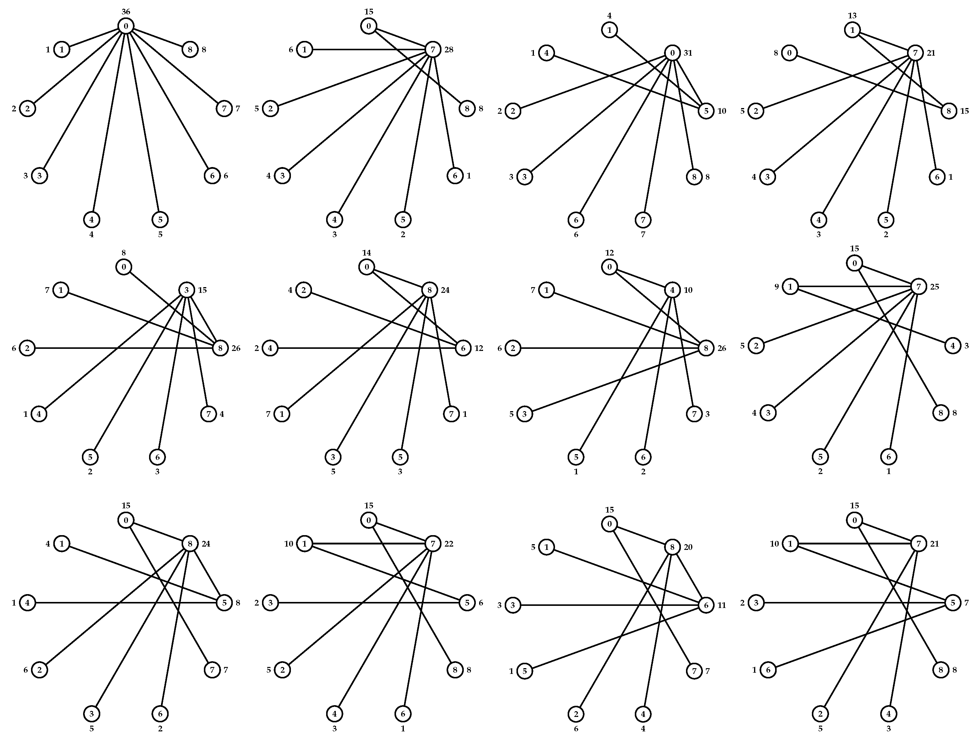
3. Summary of Trees:

Let $T_n$ denote the number of non-isomorphic trees on n vertices; then, the graceful labeling $G{T}_n$, graceful antimagic labeling $GA{T}_n$, and graceful local antimagic $GLA{T}_n$ up to 10 vertices can be calculated.

All the possible trees up to 10 vertices are discussed in Table 1.

Table 1. Summary of trees upto 10 vertices.

n	${\mathit{T}}_{\mathit{n}}$	${\mathit{GT}}_{\mathit{n}}$	${\mathit{GAT}}_{\mathit{n}}$	${\mathit{GLAT}}_{\mathit{n}}$
3	1	1	1	1
4	2	2	1	2
5	3	3	3	3
6	6	6	4	6
7	11	11	11	11
8	23	23	23	23
9	47	47	47	47
10	106	106	106	106

In the table, the first column represents the number of vertices, the second column represents the number of possible trees, the third column represents the number of trees for which the graceful labeling GL exists, the fourth column represents the number of trees for which the graceful antimagic labeling GAL exists, and the fifth column represents the number of trees in which most of the vertices share the same weights.

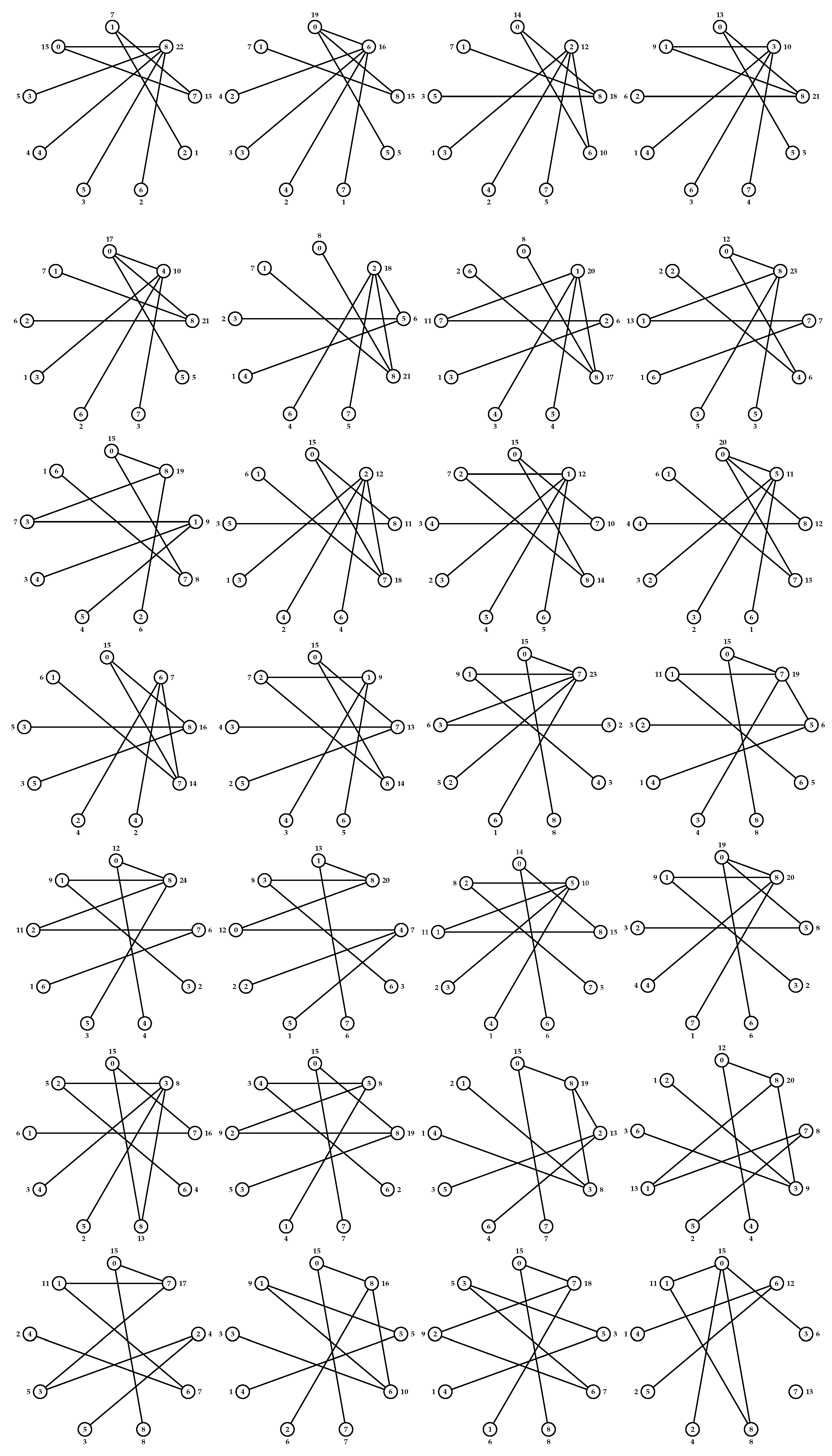
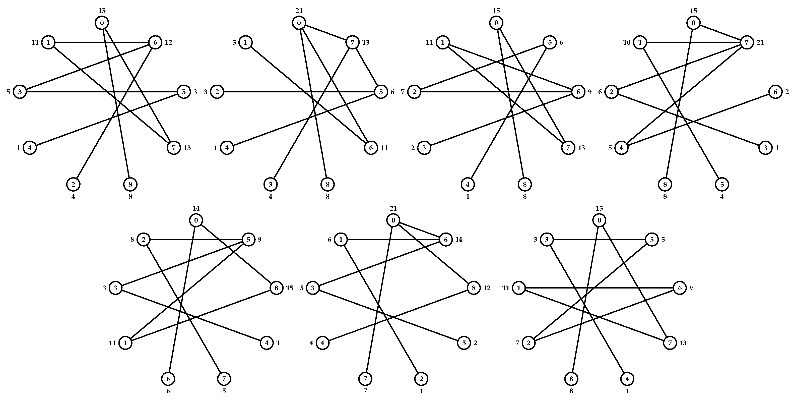
4. Summary of Path Graph

Let $GL$ denote all nonsymmetric graceful labelings of the paths on n vertices, $GAL$ graceful antimagic labeling, $GLAL$ graceful local antimagic, and $MGLAL$ minimum graceful local antimagic labelings (most of the vertices have the same weight). Table 2 summarizes the path graphs with up to 12 vertices.

Table 2. Summary of paths upto 12 vertices.

n	$\mathit{GL}$	$\mathit{GAL}$	$\mathit{GLAL}$	$\mathit{MGLAL}$
3	1	1	1	1
4	1	0	1	1
5	2	1	2	1
6	6	0	6	1
7	8	2	8	1
8	10	2	10	1
9	30	4	30	1
10	74	5	74	2
11	162	8	162	9
12	332	9	332	4

In the table, the first column represents the number of vertices, the second column represents all GLs, the third column represents the GALs, the fourth column represents GLALs, and the fifth column represents the number of GLALs in which most of the vertices share the same weight. Regarding the chromatic number of GLA labelings, up to 12 vertices can be observed.

In Table 3, the graceful local antimagic labelings for paths with up to 14 vertices are presented. These labels provide the minimum number of colors needed, which can be used to determine the chromatic number of paths.

Table 3. Graceful local antimagic labelings of paths upto 14 vertices.

n	$\mathit{f}\left({\mathit{v}}_1\right),\mathit{f}\left({\mathit{v}}_2\right),\mathit{f}\left({\mathit{v}}_3\right),\mathit{\dots },\mathit{f}\left({\mathit{v}}_{\mathit{n}-1}\right),\mathit{f}\left({\mathit{v}}_{\mathit{n}}\right)$
3	0, 2, 1
4	0, 3, 1, 2
5	1, 2, 4, 0, 3
6	1, 4, 0, 5, 3, 2
7	1, 6, 0, 4, 3, 5, 2
8	1, 6, 0, 7, 3, 4, 2, 5
9	1, 7, 0, 8, 3, 4, 6, 2, 5
10	1, 8, 0, 9, 3, 6, 2, 7, 5, 4
	2,  7, 1, 8, 0, 9, 5, 4, 6, 3
11	1, 8, 2, 10, 0, 9, 4, 5, 7, 3, 6
	1, 10, 0, 8, 3, 9, 2, 6, 5, 7, 4
	2, 8, 3, 10, 0, 9, 1, 5, 6, 4, 7
	2, 9, 1, 10, 0, 6, 5, 3, 8, 4, 7
	2, 9, 3, 8, 0, 10, 1, 5, 6, 4, 7
	3, 10, 0, 9, 1, 4, 8, 2, 7, 5, 6
	4, 1, 9, 0, 10, 3, 7, 2, 8, 6, 5
	4, 2, 8, 3, 6, 7, 0, 10, 1, 9, 5
	4, 6, 3, 7, 8, 2, 9, 1, 10, 0, 5
12	1, 10, 0, 11, 3, 8, 2, 9, 5, 6, 4, 7
	2, 9, 1, 10, 0, 11, 5, 6, 8, 3, 7, 4
	2, 9, 3, 8, 0, 11, 1, 10, 6, 5, 7, 4
	3, 11, 0, 10, 1, 5, 6, 8, 2, 9, 4, 7
13	2, 11, 3, 10, 0, 12, 1, 7, 6, 4, 9, 5, 8
	3, 8, 6, 9, 5, 4, 10, 2, 11, 1, 12, 0, 7
14	2, 11, 3, 10, 0, 13, 1, 12, 6, 7, 9, 4, 8, 5

The labeling of paths where we obtain minimum number of colors that correspond to the graceful local antmagic Chromatic number ${\chi }_{gla}$, as shown in Figure 2, Figure 3, Figure 4, Figure 5, Figure 6, Figure 7, Figure 8, Figure 9, Figure 10 and Figure 11.

Path of five vertices:

Figure 2. Graceful local antimagic labeling of 5 vertces.

Path of six vertices:

Figure 3. Graceful local antimagic labeling of 6 vertces.

Path of seven vertices:

Figure 4. Graceful local antimagic labeling of 7 vertces.

Path of eight vertices:

Figure 5. Graceful local antimagic labeling of 8 vertces.

Path of nine vertices:

Figure 6. Graceful local antimagic labeling of 9 vertces.

Path of ten vertices:

Figure 7. Graceful local antimagic labeling of 10 vertces.

Path of eleven vertices:

Figure 8. Graceful local antimagic labeling of 11 vertces.

Path of twelve vertices:

Figure 9. Graceful local antimagic labeling of 12 vertces.

Paths of thirteen vertices:

Figure 10. Graceful local antimagic labelings of 13 vertces.

Paths of fourteen vertices:

Figure 11. Graceful local antimagic labelings of 14 vertces.

$$\begin{array}{cc}\hfill & {\chi }_{gla}\left(P_3\right)={\chi }_{gla}\left(P_4\right)=3,{\chi }_{gla}\left(P_5\right)={\chi }_{gla}\left(P_6\right)={\chi }_{gla}\left(P_7\right)={\chi }_{gla}\left(P_8\right)=4,\hfill \\ \hfill & {\chi }_{gla}\left(P_9\right)=5,{\chi }_{gla}\left(P_{10}\right)=6,{\chi }_{gla}\left(P_{11}\right)={\chi }_{gla}\left(P_{12}\right)={\chi }_{gla}\left(P_{13}\right)={\chi }_{gla}\left(P_{14}\right)=7\hfill \end{array}$$

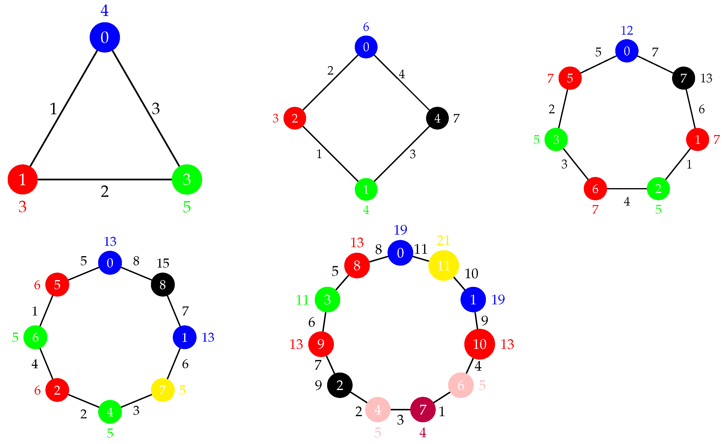
5. Summary of Cycle Graph

In Table 4, the graceful local antimagic labelings for cycles with up to 11 vertices are presented. These labels provide the minimum number of colors needed, which can be used to derive the chromatic number of cycles.

Table 4. Summary of graceful local antimagic labelings upto 11 vertices.

n	$\mathit{f}\left({\mathit{v}}_1\right),\mathit{f}\left({\mathit{v}}_2\right),\mathit{f}\left({\mathit{v}}_3\right),\mathit{\dots },\mathit{f}\left({\mathit{v}}_{\mathit{n}-1}\right),\mathit{f}\left({\mathit{v}}_{\mathit{n}}\right)$
3	0, 1, 3
4	0, 2, 1, 4
7	0, 5, 3, 6, 2, 1, 7
8	0, 5, 6, 2, 4, 7, 1, 8
11	0, 8, 3, 9, 2, 4, 7, 6, 10, 1, 11

The labeling of the cycle in which we obtained the minimum number of colors, as shown in Figure 12:

$${\chi }_{gla}\left(C_3\right)=3, {\chi }_{gla}\left(C_4\right)=4,{\chi }_{gla}\left(C_7\right)=4,{\chi }_{gla}\left(C_8\right)=5,{\chi }_{gla}\left(C_{11}\right)=7.$$

Figure 12. Graceful local antimagic labeling of cycles.

In [15], Ahmed et al. list all graceful antimagic labelings of trees with up to eight vertices. Computationally, we determined that all trees of nine vertices have a graceful antimagic labelings, which are listed in Figure 13:

Figure 13. All graceful antimagic trees on 9 vertices.

Theorem 1.

The double star $S_{n,m}$ is the graceful local antimagic for $n,m\in \mathbb{N},n\ne 1$.

Proof. 

Since $S_{2,2}\cong P_4$ and $P_4$ is the graceful local antimagic under the vertex labelings:

According to [15], $S_{n,m},(n,m)\ne (2,2)$ are graceful antimagic, which implies that $S_{n,m},(n,m)\ne (2,2)$ are graceful local antimagic, as shown in Figure 14, which completes the proof. □

Figure 14. Graceful local antimagic labeling of $P_4$.

6. Conclusions

In this research, we introduced and explored the concept of graceful local antimagic labeling for various families of graphs, utilizing Python-based algorithms as computational tools. The proposed algorithms provided a systematic approach to generating and refining graph labelings, enabling the identification of graceful, graceful antimagic, and graceful local antimagic labelings. Furthermore, we extended this analysis to compute the chromatic number of graphs by identifying labelings where the maximum number of vertices share the same weights.

References

- Chartrand, G.; Zhang, P. Introduction to Graph Theory; McGraw-Hill: New York, NY, USA, 2005. [Google Scholar]
- Wallis, W.D. Magic Graphs; Birkhäuser: Boston, MA, USA; Basel, Switzerland; Berlin, Germany, 2001. [Google Scholar]
- Kotzig, A.; Rosa, A. Magic valuations of finite graphs. Canad. Math. Bull. 1970, 13, 451–461. [Google Scholar] [CrossRef]
- Golomb, S.W. Labeling of graphs. In Recent Progress in Combinatorics; Academic Press: Cambridge, MA, USA, 1973; pp. 155–166. [Google Scholar]
- Ringel, G. Problem 25, in Theory of graphs and its applications, Proc. Symposium Smolenice. Prague 1964, 1963, 162. [Google Scholar]
- Lee, S.M.; Shee, S.C. On Skolem graceful graphs. Discrete Math. 1991, 93, 195–200. [Google Scholar] [CrossRef]
- Maheo, M.; Thuillier, H. On d-graceful graphs. Ars Combin. 1982, 13, 181–192. [Google Scholar]
- Maheo, M. Strongly graceful graphs. Discrete Math. 1980, 29, 39–46. [Google Scholar] [CrossRef]
- Slater, P.J. On k-graceful graphs. In Proceedings of the 13th SEICCGTC 1982, Boca Raton, FL, USA, 15–17 February 1982; pp. 53–57. [Google Scholar]
- Truszczynski, M. Graceful unicyclic graphs. Demonstr. Math. 1984, 17, 377–387. [Google Scholar] [CrossRef]
- Gallian, J.A. A Dynamic Survey of Graph Labeling. Electron. J. Combin. 2011, 18, 1–623. [Google Scholar] [CrossRef] [PubMed]
- Buratti, M.; Traetta, T. 2-Starters, Graceful Labelings, and a Doubling Construction for the Oberwolfach Problem. J. Combin. Des. 2012, 20, 483–503. [Google Scholar] [CrossRef]
- Burgess, A.C.; Danziger, P.; Traetta, T. On the Oberwolfach problem for single-flip 2-factors via graceful labelings. J. Comb. Theory A 2022, 189, 105–611. [Google Scholar] [CrossRef]
- Hartsfield, N.; Ringel, G. Supermagic and antimagic graphs. J. Recreat. Math. 1989, 21, 107–115. [Google Scholar]
- Ahmed, M.A.; Semaničová-Feňovčíková, A.; Bača, M.; Babujee, B.J.; Shobana, L. On graceful antimagic graphs. Aequat. Math. 2023, 97, 13–30. [Google Scholar] [CrossRef]
- Hartsfield, N.; Ringel, G. Pearls in Graph Theory; Academic Press, Inc.: Boston, MA, USA, 1994. [Google Scholar]
- Cranston, D.W.; Liang, Y.C.; Zhu, X. Regular graphs of odd degree are antimagic. J. Graph Theory 2015, 80, 28–33. [Google Scholar] [CrossRef]
- Bača, M.; Miller, M.; Phanalasy, O.; Semaničová-Feňovčíková, A. Antimagic labelings of join graphs. Math. Comput. Sci. 2015, 9, 139–143. [Google Scholar] [CrossRef]
- Arumugam, S.; Premalatha, K.; Bača, M.; Semaničová-Feňovčíková, A. Local antimagic vertex coloring of a graph. Graphs Combin. 2017, 33, 275–285. [Google Scholar] [CrossRef]
- Haslegrave, J. Proof of a local antimagic conjecture. Discr. Math. Theor. Comp. Sci. 2018, 20, 1–14. [Google Scholar]
Disclaimer/Publisher’s Note: The statements, opinions and data contained in all publications are solely those of the individual author(s) and contributor(s) and not of MDPI and/or the editor(s). MDPI and/or the editor(s) disclaim responsibility for any injury to people or property resulting from any ideas, methods, instructions or products referred to in the content. |
© 2025 by the authors. Licensee MDPI, Basel, Switzerland. This article is an open access article distributed under the terms and conditions of the Creative Commons Attribution (CC BY) license (https://creativecommons.org/licenses/by/4.0/).