Improving Influenza Epidemiological Models under Caputo Fractional-Order Calculus

Abstract

The Caputo fractional-order differential operator is used in epidemiological models, but its accuracy benefits are typically ignored. We validated the suggested fractional epidemiological seasonal influenza model of the SVEIHR type to demonstrate the Caputo operator’s relevance. We analysed the model using fractional calculus, revealing its basic properties and enhancing our understanding of disease progression. Furthermore, the positivity, bounds, and symmetry of the numerical scheme were examined. Adjusting the Caputo fractional-order parameter $\mathsf{\alpha }$ = 0.99 provided the best fit for epidemiological data on infection rates. We compared the suggested model with the Caputo fractional-order system and the integer-order equivalent model. The fractional-order model had lower absolute mean errors, suggesting that it could better represent sickness transmission and development. The results underline the relevance of using the Caputo fractional-order operator to improve epidemiological models’ precision and forecasting. Integrating fractional calculus within the framework of symmetry helps us build more reliable models that improve public health interventions and policies.

1. Introduction

Influenza was not considered a particularly dangerous infection prior to the First World War. The most catastrophic influenza pandemic [1,2] impacted everything, and the danger of such a disaster occurring again was the primary reason for the restriction to all subsequent progress.

Influenza is an extremely contagious disease caused by influenza viruses. This illness is characterised by a wide range of symptoms, each with varying severity [3,4]. Symptoms may include fever, runny nose, sore throat, muscle soreness, headache, cough, and exhaustion. Symptoms usually begin within one to four days after exposure to the virus and can last for two to eight days [5]. Sometimes diarrhoea and vomiting occur, especially in children. Pneumonia often follows influenza or a bacterial infection. Patients may develop acute respiratory distress syndrome, meningitis, encephalitis, and asthma or cardiovascular disease aggravation.

Influenza viruses are divided into four different types [6,7]: A, B, C, and D. Influenza A virus commonly infects waterfowl and can also infect a variety of mammals, such as humans and pigs. Influenza B virus and influenza C virus mainly infect humans, while influenza D virus affects cattle and pigs. Human influenza A and B viruses cause seasonal epidemics. Coughing and sneezing spread influenza viruses. Surfaces and aerosols polluted with viruses are more likely to transmit infection.

The World Health Organisation classifies influenza as a serious illness that can lead to hospitalisation and sometimes death. Every flu season is different, and influenza infection can affect people differently. Even healthy people can become severely ill with the flu and spread it to others. The burden of influenza was estimated from surveillance data in Saudi Arabia [8] using epidemiological parameters of transmission using classical WHO tools and mathematical modelling.

Mathematical models (MMs) of influenza virus infection kinetics depend mainly on ordinary differential equations (ODEs) that describe the temporal evolution of infection (the virus as a function of time), which has been discussed in several reviews [9,10,11,12]. To predict the global spread of influenza, a mathematical model was used based on information from the first city in the transportation network to be exposed to the disease [13], where the model formulation was given along with a method for estimating critical parameters. In [14], a mathematical model was formulated to analyse the transmission dynamics of the influenza A virus, which included the aspect of drug resistance. The model balances were calculated, and stability analysis was performed. Numerical simulations revealed that, although vaccination reduced the number of infections, influenza was still present in the population. Therefore, in addition to vaccination, it was necessary to apply other strategies to reduce the spread of influenza. A compartmental model with a time-varying contact rate, the seasonality effect, and the corresponding nonautonomous model were studied in [15]. The model was simulated using the RK-45 numerical approach. Every day, fractional calculus and its explanations gain popularity globally. We have devised new fractional operators with varied features to mimic real-world issues. Widely researched epidemiological models of infectious illnesses use integer-order differential equations. Mathematical epidemic modelling suggests that nonlinear dynamical equations may reveal illness transmission patterns. Many studies, including those that use Caputo and other memory operators [16], have used data-driven, nonlinear compartmental mathematical models to explain how seasonal influenza spreads. Ref. [17] provides a new method for modelling influenza by studying illness dynamics using the CF fractional derivative operator. Yavuz et al. [18] adopted the exponential law kernel and Mittag-Leffler kernel inside the framework of the Caputo fractional derivative.

Farman et al. [19]. conducted a study that examined the epidemiological analysis of a COVID-19 model employing a fractional order and Mittag-Leffler kernel. Joshi and Jha [20] developed a mathematical model to study the movement of calcium inside cells, with a particular focus on Parkinson’s disease. The researchers used the Hilfer fractional reaction–diffusion equation for their inquiry [21]. In their 2016 study, Bonyah et al. conducted research on the topic of listeriosis illness using fractal-fractional operators. Kumar and Erturk conducted a study on the dynamics of cholera using two separate numerical methods that relied on fractional order. The benefits of fractional differential equations were highlighted in their application to memory trace and hereditary traits [22].

The paper by Caputo and Fabrizio [23] deployed the notion of “memory trace” to elucidate the impact of previous infections on the current epidemic. The memory effects inside the system were modelled using a fractional-order model. The study conducted by Fatma and Yavuz [24,25] explored the differentiation between the Markov term and the memory trace, which may be seen as the resolution to fractional-order differential equations. Asifa et al. [26] utilised the nonlocal nature of the Caputo differential operator to fractionate the SAIVR epidemic model of order $\alpha$. This approach allowed for the investigation of the COVID-19 pandemic by incorporating memory traces and hereditary traits, which demonstrated the model’s vanishing behaviour.

Through the integration of fractional and classical models, this study improves influenza modelling and forecasting. The following aspects contribute to the uniqueness of this study:

• This study combines classical and fractional differential equations to enhance compartmental models. This study enhances our comprehension of the dynamics of influenza virus transmission and the impact of vaccination and resistance to therapy.
• It uses fractional calculus and the Caputo operator to simulate the effects of influenza memory. This novel approach captures the disease’s nonlocal behaviour and genetic characteristics, providing insights that cannot be obtained with integer-order differential equations.
• The study utilises Saudi Arabian surveillance data and uses WHO epidemiological parameter estimation methodologies to develop its models. This enhances the relevance of the outcomes to the design and implementation of public health measures.
• The study examines the transmission patterns and evaluates the impact of vaccination and other control measures on the spread of influenza. Stability studies and computer simulations indicate that relying just on vaccination is inadequate for controlling the sickness, and other techniques are necessary.
• Fractional differential operators include memory traces and genetic characteristics, offering a novel technique for simulating illnesses. This methodology elucidates the impact of previous infections on epidemic patterns and facilitates the development of more effective long-term intervention strategies. This advancement enhances the understanding of fractional derivatives in the field of epidemiology. This study integrates traditional and fractional calculus methodologies to model influenza dynamics uniquely. It supports public health planning and research on infectious disease models.

2. Preliminaries

Definition 1

([27]). The Riemann–Liouville fractional integral of a function $g:{\mathbb{R}}^{+}\to \mathbb{R}$ with order $\alpha >0$ is defined as

$$I_{0^{+}}^{\alpha }\left(g\left(t\right)\right)={\displaystyle \frac{1}{\mathsf{\Gamma }\left(\alpha \right)}}{\int }_0^t{(t-\omega )}^{\alpha -1}g\left(\omega \right)d\omega ,t>0,$$

(1)

where $\mathsf{\Gamma }\left(\alpha \right)$ is the Euler’s gamma function.

Definition 2

([27]). The Riemann–Liouville fractional differential operator for a function $g\left(t\right)$ with order $\alpha >0$ is defined as

$${\mathbb{D}}_{0^{+}}^{\alpha }\left(g\left(t\right)\right)={\displaystyle \frac{1}{\mathsf{\Gamma }(m-\alpha )}}{\displaystyle \frac{d^m}{d{t}^m}}\left({\int }_0^t{(t-\omega )}^{m-\alpha -1}g\left(\omega \right)d\omega \right),t>0,$$

(2)

where $m-1<\alpha <m$, $m\in \mathbb{N}$.

Definition 3

([28]). The fractional-order derivative of a function $g\left(t\right)$ based upon the Caputo definition with order $\alpha >0$ is given by

$${ }^C{\mathbb{D}}_{0^{+}}^{\alpha }\left(g\left(t\right)\right)={\displaystyle \frac{1}{\mathsf{\Gamma }(m-\alpha )}}{\int }_0^t{(t-\omega )}^{m-\alpha -1}{g}^{\left(m\right)}\left(\omega \right)d\omega ,t>0,$$

(3)

where $m-1<\alpha <m$, $m\in \mathbb{N}$.

Lemma 1

([28]). Let $g(t,x)$ be a real-valued continuous function. Consider the system

$${ }^C{D}_{t_0}^{q}x\left(t\right)=g(t,x),t>t_0,$$

where $q\in (0,1)$, with initial condition $x\left(t_0\right)$. If $g(t,x)$ in (2) satisfies the locally Lipschitz condition with respect to x, then there exists a unique solution of system (2) on $[t_0,+\infty )\times \mathsf{\Omega }$ and $\mathsf{\Omega }\subset {\mathbb{R}}^n$.

Lemma 2

([28]). Let $x\left(t\right)\in {\mathbb{R}}^{+}$ be a continuous and derivable function. Then,

$${ }^C{D}_{t_0}^q\left(x\left(t\right)-x^{*}-x^{*}ln{\displaystyle \frac{x\left(t\right)}{x^{*}}}\right)\le \left(1-{\displaystyle \frac{x^{*}}{x\left(t\right)}}\right){ }^C{D}_{t_0}^{q}x\left(t\right),$$

where $t\ge t_0$, $q\in (0,1)$, and $x^{*}\in {\mathbb{R}}^{+}$.

Lemma 3

([29]). Let $t>0$, $n-1<\alpha \le n$, $n\in \mathbb{N}$. Then, the following relations hold:

$${ }_{t_0}{D}_t^{\alpha }g\left(t\right)={ }_{t_0}^C{D}_t^{\alpha }g\left(t\right)+\sum _{k=0}^{n-1}{\displaystyle \frac{g^{\left(k\right)}\left(t_0\right)}{\mathsf{\Gamma }(k-\alpha +1)}}{(t-t_0)}^{k-\alpha },$$

$${ }_{t_0}{D}_t^{\alpha }g\left(t\right)={ }_{t_0}^C{D}_t^{\alpha }g\left(t\right)+\sum _{k=0}^{n-1}{\displaystyle \frac{g^{\left(k\right)}\left(T\right)}{\mathsf{\Gamma }(k-\alpha +1)}}{(T-t)}^{k-\alpha },$$

therefore, if $g\left(t_0\right)=g^{\prime }\left(t_0\right)=g^{″}\left(t_0\right)=\dots =g^{(n-1)}\left(t_0\right)=0$, then ${ }_{t_0}{D}_t^{\alpha }g\left(t\right)={ }_{t_0}^C{D}_t^{\alpha }g\left(t\right)$, if $g\left(T\right)=g^{\prime }\left(T\right)=g^{″}\left(T\right)=\dots =g^{(n-1)}\left(T\right)=0$, then ${ }_{t_0}{D}_t^{\alpha }g\left(t\right)={ }_{t_0}^C{D}_t^{\alpha }g\left(t\right)$, where ${ }_{t_0}^C{D}_t^{\alpha }$ is the Caputo fractional derivative, and ${ }_{t_0}{D}_t^{\alpha }$ is the Riemann–Liouville derivative.

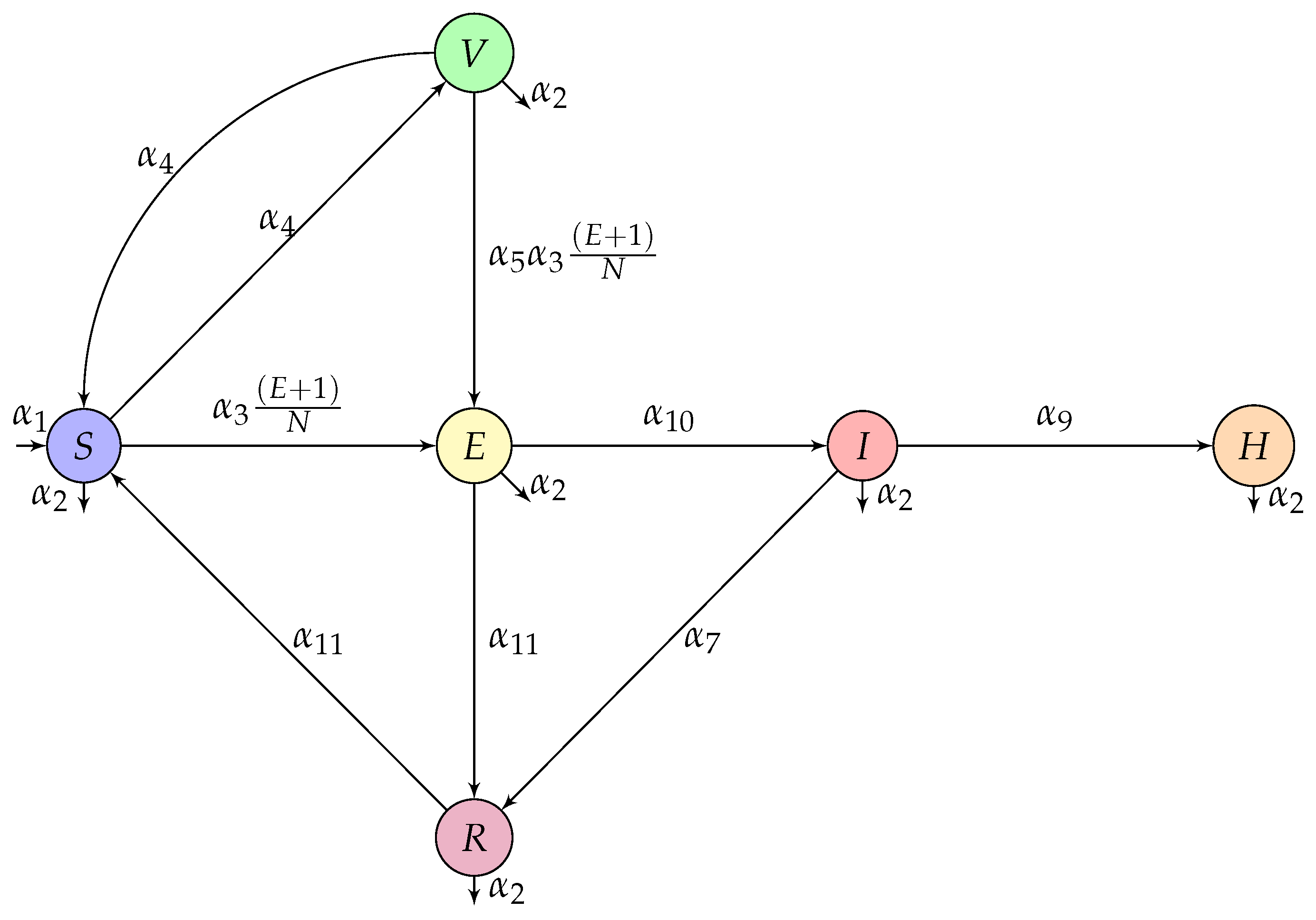
3. Model Construction

The transmission dynamic of influenza is modelled using a deterministic SEIHR-V model with susceptible (S), exposed (E), infectious (I), hospitalized (H), recovered (R), and vaccinated (V) compartments ($SEIHR-V$), such that at any time t, the total population is

$$N\left(t\right)=S\left(t\right)+V\left(t\right)+E\left(t\right)+I\left(t\right)+H\left(t\right)+R\left(t\right).$$

Each class incurs a fixed natural death at rate ${\alpha }_2$. The susceptible class is assumed to be increasing by recruitment processes at rate ${\alpha }_1$ and by waning immunity of the individuals in classes V and R at rate ${\alpha }_{11}$, and decreasing by vaccination at rate ${\alpha }_4$ and by the force of the infection

$$f_1={\alpha }_3{\displaystyle \frac{(E+I)S}{N}},$$

where ${\alpha }_5$ is the vaccination inefficacy (i.e., $1-{\alpha }_5$ is the vaccine efficacy), and ${\alpha }_3$ is the probability of an individual in class S or V being infected with the disease after coming in contact with an infected or exposed person. Individuals in class V are recruited from class S at rate ${\alpha }_4$. Vaccination does not confer a long-lasting immunity nor the full protection is guaranteed. Therefore, vaccinated individuals become susceptible again at rate ${\alpha }_{11}$ due to waning immunity and exposition to the virus by the force of the infection

$$f_2={\alpha }_5{\alpha }_3{\displaystyle \frac{(E+I)V}{N}}.$$

Individuals in class E are recruited by the forces of the infection $f_1$ and $f_2$, move to class I at rate ${\alpha }_{10}$ (after the incubation period) and to class R at rate ${\alpha }_8$. Infected individuals are recruited with rate ${\alpha }_{10}$ from class E, recover at rate ${\alpha }_7$, and an ${\alpha }_6$ fraction of them become hospitalized. The recovered population is increased from classes $E,I$, and H at rates ${\alpha }_8,{\alpha }_7,$ and ${\alpha }_9$, respectively, and become susceptible again at rate ${\alpha }_{11}$.

From the above description, we derived system (4) of fractional differential equations to mathematically describe the transmission dynamics of influenza as described in Figure 1.

$$\begin{array}{c}\hfill \begin{array}{cc}\hfill { }^C{\mathcal{D}}_{0,t}^{\alpha }S\left(t\right)=& {\alpha }_1+{\alpha }_{11}(V+R)-{\alpha }_3{\displaystyle \frac{(E+I)S}{N}}-({\alpha }_4+{\alpha }_2)S\hfill \\ \hfill { }^C{\mathcal{D}}_{0,t}^{\alpha }V\left(t\right)=& {\alpha }_{4}S-{\alpha }_5{\alpha }_3{\displaystyle \frac{(E+I)V}{N}}-({\alpha }_{11}+{\alpha }_2)V\hfill \\ \hfill { }^C{\mathcal{D}}_{0,t}^{\alpha }E\left(t\right)=& {\alpha }_3{\displaystyle \frac{(E+I)(S+{\alpha }_{5}V)}{N}}-({\alpha }_{10}+{\alpha }_8+{\alpha }_2)E\hfill \\ \hfill { }^C{\mathcal{D}}_{0,t}^{\alpha }I\left(t\right)=& {\alpha }_{10}E-({\alpha }_7+{\alpha }_6+{\alpha }_2)I\hfill \\ \hfill { }^C{\mathcal{D}}_{0,t}^{\alpha }H\left(t\right)=& {\alpha }_{6}I-({\alpha }_9+{\alpha }_2)H\hfill \\ \hfill { }^C{\mathcal{D}}_{0,t}^{\alpha }R\left(t\right)=& {\alpha }_{8}E+{\alpha }_{7}I+{\alpha }_{9}H-({\alpha }_{11}+{\alpha }_2)R,\hfill \end{array}\end{array}$$

(4)

with initial conditions $S\left(0\right)=S_0\ge 0,V\left(0\right)=V_0\ge 0,E\left(0\right)=E_0\ge 0,I\left(0\right)=I_0\ge 0, H\left(0\right)=H_0\ge 0,$ and $R\left(0\right)=R_0\ge 0.$

Table 1. Description of the parameters of model (4).

Parameter	Description	Value	Source
${\alpha }_1$	Recruitment rate of individuals into the population	0.114	Fitted
${\alpha }_2$	Natural death rate	0.000256	[8]
${\alpha }_3$	Average effective contact rate	0.858	Fitted
${\alpha }_4$	Vaccination rate	0.114	Fitted
${\alpha }_5$	Vaccine inefficacy	1.00	Fitted
${\alpha }_6$	Average hospitalization rate	0.0015	Fitted
${\alpha }_7$	Recovery rate for infected individuals	2.6	Fitted
${\alpha }_8$	Recovery rate for exposed individuals	0.34	Fitted
${\alpha }_9$	Recovery rate for hospitalized individuals	0.68	Fitted
${\displaystyle \frac{1}{{\alpha }_{10}}}$	Average latent or incubation period	1.6 day	[30]
${\alpha }_{11}$	Rate at which individuals lose immunity	50 days	[8]

provides full descriptions, values, and information on all model parameters. Model (4) was fitted using influenza data from the Ministry of Health of the Kingdom of Saudi Arabia for 2021 [8].

The analysis of integer-order deterministic models employs a characteristic fractional-order operator. We used the Caputo type operator to perform a fractional evaluation of the influenza epidemic mode. The basis for this evaluation was the existence of solutions and the use of this type of operator for nonlinear differential equations. There has been a rise in popularity of the Caputo fractional operator as a result of its widespread application in epidemiological modelling. The Caputo operator represents nonlinear differential equations, where alpha signifies the fractional-order operator in the context of understanding the Caputo operator.

The purpose of this research was to investigate the use of fractional calculus in mathematical epidemiology, specifically for the purpose of developing a model of influenza, among other various uses [31]. To be more specific, fractional derivative formulations were utilised in order to accurately simulate the infectious disease systems in question. Indeed, fractional-order differential equation systems are attractive epidemiological models. These systems provide memory effects and more degrees of freedom; thus, this is expected. In reality, the fractional-order derivative can express the memory and heredity of many materials and processes. Fractional differential equations are better at representing nonlocal events than integer-order derivatives. The failure of classical first-order differential equations to properly duplicate statistical data from a genuine disease outbreak shows that this traditional model rarely produces satisfactory or desirable results. We studied a more accurate and sophisticated fractional differential equation collection to improve outcomes.

4. Analysis of the Model

In this section, we examine some dynamical aspects of model (4) to understand under what conditions the disease becomes persistent or extinct in a population.

4.1. Existence and Uniqueness

Theorem 1.

For each non-negative initial condition $(S_0,V_0,E_0,I_0,Q_0,R_0,D_0)\in {\mathbb{R}}^7$, there exists a unique solution of fractional model (5).

Proof. 

Let $\mathsf{\Omega }=\{(S,V,E,I,Q,R,D)\in {\mathbb{R}}^7:max\left\{\right|S|,|V|,|E|,|I|,|Q|,|R|,|D\left|\right\}\le \rho \}$. Define a mapping $M\left(X\right)=(M_1\left(X\right),M_2\left(X\right),M_3\left(X\right),M_4\left(X\right),M_5\left(X\right),M_6\left(X\right),M_7\left(X\right))$, and

$$\begin{array}{cc}\hfill M_1\left(X\right)& ={\alpha }_1+{\alpha }_{11}(V+R)-{\alpha }_3{\displaystyle \frac{(E+I)S}{N}}-({\alpha }_4+{\alpha }_2)S,\hfill \\ \hfill M_2\left(X\right)& ={\alpha }_{4}S-{\alpha }_{13}{\displaystyle \frac{(E+I)V}{N}}-({\alpha }_{11}+{\alpha }_2)V,\hfill \\ \hfill M_3\left(X\right)& ={\alpha }_3{\displaystyle \frac{(E+I)(S+{\alpha }_{5}V)}{N}}-({\alpha }_{10}+{\alpha }_8+{\alpha }_2)E,\hfill \\ \hfill M_4\left(X\right)& ={\alpha }_{10}E-({\alpha }_7+{\alpha }_6+{\alpha }_2)I,\hfill \\ \hfill M_5\left(X\right)& ={\alpha }_{6}I-({\alpha }_9+{\alpha }_2)H,\hfill \\ \hfill M_6\left(X\right)& ={\alpha }_{8}E+{\alpha }_{7}I+{\alpha }_{9}H-({\alpha }_{11}+{\alpha }_2)R,\hfill \end{array}$$

where $X=(S,V,E,I,H,R)\in \mathsf{\Omega }$.

For any $X,\tilde{X}\in \mathsf{\Omega }$, we have

$$\begin{array}{cc}\hfill \parallel M\left(X\right)-M\left(\tilde{X}\right)\parallel & =\parallel M_1\left(X\right)-M_1\left(\tilde{X}\right)\parallel +\parallel M_2\left(X\right)-M_2\left(\tilde{X}\right)\parallel +\parallel M_3\left(X\right)-M_3\left(\tilde{X}\right)\parallel \hfill \\ & +\parallel M_4\left(X\right)-M_4\left(\tilde{X}\right)\parallel +\parallel M_5\left(X\right)-M_5\left(\tilde{X}\right)\parallel +\parallel M_6\left(X\right)-M_6\left(\tilde{X}\right)\parallel \hfill \\ & \le \left|{\alpha }_1+{\alpha }_{11}(V+R)-{\alpha }_3{\displaystyle \frac{(E+I)S}{N}}-({\alpha }_4+{\alpha }_2)S\right.\hfill \\ & \left.-{\alpha }_1-{\alpha }_{11}(\tilde{V}+\tilde{R})+{\alpha }_3{\displaystyle \frac{(E+I)\tilde{S}}{N}}+({\alpha }_4+{\alpha }_2)\tilde{S}\right|\hfill \\ & +\left|{\alpha }_{4}S-{\alpha }_{13}{\displaystyle \frac{(E+I)V}{N}}-({\alpha }_{11}+{\alpha }_2)V\right.\hfill \\ & \left.-{\alpha }_4\tilde{S}+{\alpha }_{13}{\displaystyle \frac{(E+I)\tilde{V}}{N}}+({\alpha }_{11}+{\alpha }_2)\tilde{V}\right|\hfill \\ & +\left|{\alpha }_3{\displaystyle \frac{(E+I)(S+{\alpha }_{5}V)}{N}}-({\alpha }_{10}+{\alpha }_8+{\alpha }_2)E\right.\hfill \\ & \left.-{\alpha }_3{\displaystyle \frac{(\tilde{E}+\tilde{I})(\tilde{S}+{\alpha }_5\tilde{V})}{N}}+({\alpha }_{10}+{\alpha }_8+{\alpha }_2)\tilde{E}\right|\hfill \\ & +\left|{\alpha }_{10}E-({\alpha }_7+{\alpha }_6+{\alpha }_2)I-{\alpha }_{10}\tilde{E}+({\alpha }_7+{\alpha }_6+{\alpha }_2)\tilde{I}\right|\hfill \\ & +\left|{\alpha }_{6}I-({\alpha }_9+{\alpha }_2)H-{\alpha }_6\tilde{I}+({\alpha }_9+{\alpha }_2)\tilde{H}\right|\hfill \\ & +\left|{\alpha }_{8}E+{\alpha }_{7}I+{\alpha }_{9}H-({\alpha }_{11}+{\alpha }_2)R\right.\hfill \\ & \left.-{\alpha }_8\tilde{E}-{\alpha }_7\tilde{I}-{\alpha }_9\tilde{H}+({\alpha }_{11}+{\alpha }_2)\tilde{R}\right|\hfill \\ & \le (2{\alpha }_3+{\alpha }_4+{\alpha }_2)|S-\tilde{S}|\hfill \\ & +(2{\alpha }_{13}+{\alpha }_{11}+{\alpha }_2)|V-\tilde{V}|\hfill \\ & +(2{\alpha }_3+{\alpha }_{10}+{\alpha }_8+{\alpha }_2)|E-\tilde{E}|\hfill \\ & +({\alpha }_{10}+{\alpha }_7+{\alpha }_6+{\alpha }_2)|I-\tilde{I}|\hfill \\ & +({\alpha }_6+{\alpha }_9+{\alpha }_2)|H-\tilde{H}|\hfill \\ & +({\alpha }_8+{\alpha }_7+{\alpha }_9+{\alpha }_{11}+{\alpha }_2)|R-\tilde{R}|\hfill \\ & \le L\parallel X-\tilde{X}\parallel ,\hfill \end{array}$$

where L = max 2${\alpha }_3$ + ${\alpha }_4$ + ${\alpha }_2$, 2${\alpha }_{13}$ + ${\alpha }_{11}$ + ${\alpha }_2,$ 2${\alpha }_3$ + ${\alpha }_{10}$ + ${\alpha }_8$ + ${\alpha }_2$, ${\alpha }_{10}$ + ${\alpha }_7$ + ${\alpha }_6$ + ${\alpha }_2$, ${\alpha }_6$ + ${\alpha }_9$ + ${\alpha }_2,$ ${\alpha }_8$ + ${\alpha }_7$ + ${\alpha }_9$ + ${\alpha }_{11}$ + ${\alpha }_2$.

That is, $M\left(X\right)$ satisfies the Lipschitz condition. According to Lemma 1, model (4) has a unique solution. □

4.2. Boundedness and Non-Negativity

The last equation of recovered individuals $R\left(t\right)$ in system (5) is independent of other equations. System (5) can be reduced to the following form:

$$\begin{array}{cc}\hfill { }^C{\mathcal{D}}_{0,t}^{\alpha }S\left(t\right)& =a_1+a_{11}(V+R)-a_3{\displaystyle \frac{(E+I)S}{N}}-(a_4+a_2)S,\hfill \\ \hfill { }^C{\mathcal{D}}_{0,t}^{\alpha }V\left(t\right)& =a_{4}S-a_5{a}_3{\displaystyle \frac{(E+I)V}{N}}-(a_{11}+a_2)V,\hfill \\ \hfill { }^C{\mathcal{D}}_{0,t}^{\alpha }E\left(t\right)& =a_3{\displaystyle \frac{(E+I)(S+a_{5}V)}{N}}-(a_{10}+a_8+a_2)E,\hfill \\ \hfill { }^C{\mathcal{D}}_{0,t}^{\alpha }I\left(t\right)& =a_{10}E-(a_7+a_6+a_2)I,\hfill \\ \hfill { }^C{\mathcal{D}}_{0,t}^{\alpha }H\left(t\right)& =a_{6}I-(a_9+a_2)H,\hfill \\ \hfill { }^C{\mathcal{D}}_{0,t}^{\alpha }R\left(t\right)& =a_{8}E+a_{7}I+a_{9}H-(a_{11}+a_2)R.\hfill \end{array}$$

(5)

Theorem 2.

The solutions of fractional model (5) are uniformly bounded and non-negative for $t\ge 0$.

Proof. 

Let $N\left(t\right)=S\left(t\right)+V\left(t\right)+E\left(t\right)+I\left(t\right)+H\left(t\right)+R\left(t\right)$. From Equation (5), one has

$${ }^C{\mathcal{D}}_{0,t}^{\alpha }N\left(t\right)\le a_1+a_{11}(V+R)-{\alpha }_{2}N\left(t\right).$$

(6)

Using the comparison principle of fractional systems, one derives

$$N\left(t\right)\le {\displaystyle \frac{a_1+a_{11}}{{\alpha }_2}}{E}_{\alpha ,1}\left(-{\displaystyle \frac{{\alpha }_2{t}^{\alpha }}{\mathsf{\Gamma }(\alpha +1)}}\right)N\left(0\right)E_{\alpha ,1}\left(-{\displaystyle \frac{{\alpha }_2{t}^{\alpha }}{\mathsf{\Gamma }(\alpha +1)}}\right),$$

(7)

where $E_{\alpha ,1}$ is the Mittag-Leffler function. From ${lim}_{t\to \infty }{E}_{\alpha ,1}\left(-{\displaystyle \frac{{\alpha }_2{t}^{\alpha }}{\mathsf{\Gamma }(\alpha +1)}}\right)=0$, one obtains

$$N\left(t\right)\le {\displaystyle \frac{a_1+a_{11}}{{\alpha }_2}}\mathrm{as}t\to \infty .$$

Thus, all the solutions of fractional model (5) are confined to the region

$$\mathsf{\Omega }=\{(S,V,E,I,H,R)\in {\mathbb{R}}^6:N\left(t\right)\le {\displaystyle \frac{a_1+a_{11}}{{\alpha }_2}},t\ge 0\}.$$

According to the fractional comparison theorem and the properties of the Mittag-Leffler function, for any $q\in (0,1)$, one obtains

$$S\left(t\right)\ge S_0{E}_{\alpha ,1}\left(\left({\displaystyle \frac{a_1+{\alpha }_{11}}{{\alpha }_2}}+{\alpha }_4+{\alpha }_2\right)t^{\alpha }\right)\ge S\left(t\right)\ge 0.$$

Similarly, one can prove that

$$V\left(t\right)\ge V_0{E}_{\alpha ,1}\left(\left(\left({\alpha }_5\right)\left({\alpha }_3\right){\displaystyle \frac{{\alpha }_1+{\alpha }_{11}}{{\alpha }_2}}+{\alpha }_{11}+{\alpha }_2\right)t^{\alpha }\right)\ge V\left(t\right)\ge 0.$$

$$E\left(t\right)\ge E_0{E}_{\alpha ,1}\left(\left(\left({\alpha }_3\right){\displaystyle \frac{{\alpha }_1+{\alpha }_{11}}{{\alpha }_2}}+{\alpha }_{10}+{\alpha }_8+{\alpha }_2\right)t^{\alpha }\right)\ge E\left(t\right)\ge 0.$$

$$I\left(t\right)\ge I_0{E}_{\alpha ,1}\left(\left({\alpha }_7+{\alpha }_6+{\alpha }_2\right)t^{\alpha }\right)\ge I\left(t\right)\ge 0.$$

$$H\left(t\right)\ge H_0{E}_{\alpha ,1}\left(\left({\alpha }_9+{\alpha }_2\right)t^{\alpha }\right)\ge H\left(t\right)\ge 0.$$

$$R\left(t\right)\ge R_0{E}_{\alpha ,1}\left(\left({\alpha }_{11}+{\alpha }_2\right)t^{\alpha }\right)\ge R\left(t\right)\ge 0.$$

Thus, the solution of fractional model (5) is non-negative. This completes the proof. □

4.3. The Basic Reproduction Number $R_0$

In the absence of influenza, all infected model compartments remain unaffected, i.e., $E=I=H=R=0$. However, we considered the presence of vaccination even in the absence of the disease. The coordinates of the disease-free equilibrium $\left(E_{dfe}\right)$ of system (4) were obtained by setting the right-hand sides of all the equations in system (4) to zero, as follows:

$$E_{dfe}=\left(S_0^{*},V_0^{*},E_0^{*},I_0^{*},H_0^{*},R_0^{*}\right),$$

(8)

where $S_0^{*}={\displaystyle \frac{{\alpha }_1{\alpha }_{11}+{\alpha }_1{\alpha }_2}{{\alpha }_2({\alpha }_4+{\alpha }_{11}+{\alpha }_2)}},V_0^{*}={\displaystyle \frac{{\alpha }_4{\alpha }_1}{{\alpha }_2({\alpha }_4+{\alpha }_{11}+{\alpha }_2)}}$, and $E_0^{*}=I_0^{*}=H_0^{*}=R_0^{*}=0.$

The reproduction number serves as a fundamental metric in epidemiology, providing a quantitative assessment of the rate at which a disease is disseminating. In this section, we employ the next-generation operator method [32] to derive the vaccine-induced and basic reproduction numbers for system (4). Notably, within the system, there are three infected classes, namely E, I, and H, and our focus narrows down to the sub-system (9) involving these infected classes.

$$\begin{array}{ccc}\hfill { }^C{\mathcal{D}}_{0,t}^{\alpha }E\left(t\right)& =& {\alpha }_3{\displaystyle \frac{(E+I)(S+{\alpha }_{5}V)}{N}}-({\alpha }_{10}+{\alpha }_8+{\alpha }_2)E\hfill \\ \hfill { }^C{\mathcal{D}}_{0,t}^{\alpha }I\left(t\right)& =& {\alpha }_{10}E-({\alpha }_7+{\alpha }_6+{\alpha }_2)I\hfill \\ \hfill { }^C{\mathcal{D}}_{0,t}^{\alpha }H\left(t\right)& =& {\alpha }_{6}I-({\alpha }_9+{\alpha }_2)H.\hfill \end{array}$$

(9)

Then, we derive

$$f\left(x\right)=\left[\begin{array}{c}{\alpha }_3{\displaystyle \frac{(E+I)(S+{\alpha }_{5}V)}{N}}\\ 0\\ 0\end{array}\right]\mathrm{and}v\left(x\right)=\left[\begin{array}{c}({\alpha }_{10}+{\alpha }_8+{\alpha }_2)E\\ -{\alpha }_{10}E+({\alpha }_7+{\alpha }_6+{\alpha }_2)I\\ -{\alpha }_{6}I+({\alpha }_9+{\alpha }_2)H\end{array}\right].$$

The Jacobians of $f\left(x\right)$ and $v\left(x\right)$ at $E_{dfe}$ are

$$F=\left[\begin{array}{ccc}{\displaystyle \frac{{\alpha }_3(S_0^{*}+{\alpha }_5{V}_0^{*})}{N_0^{*}}}& {\displaystyle \frac{{\alpha }_3(S_0^{*}+{\alpha }_5{V}_0^{*})}{N_0^{*}}}& 0\\ 0& 0& 0\\ 0& 0& 0\end{array}\right],$$

and

$$V=\left[\begin{array}{ccc}({\alpha }_{10}+{\alpha }_8+{\alpha }_2)& 0& 0\\ -{\alpha }_{10}& ({\alpha }_7+{\alpha }_6+{\alpha }_2)& 0\\ 0& -{\alpha }_6& ({\alpha }_9+{\alpha }_2)\end{array}\right].$$

The inverse of V is

$$V^{-1}=\left[\begin{array}{ccc}{\displaystyle \frac{1}{({\alpha }_{10}+{\alpha }_8+{\alpha }_2)}}& 0& 0\\ {\displaystyle \frac{{\alpha }_{10}}{({\alpha }_{10}+{\alpha }_8+{\alpha }_2)({\alpha }_7+{\alpha }_6+{\alpha }_2)}}& {\displaystyle \frac{1}{({\alpha }_7+{\alpha }_6+{\alpha }_2)}}& 0\\ {\displaystyle \frac{{\alpha }_{10}{\alpha }_6}{({\alpha }_{10}+{\alpha }_8+{\alpha }_2)({\alpha }_7+{\alpha }_6+{\alpha }_2)({\alpha }_9+{\alpha }_2)}}& {\displaystyle \frac{{\alpha }_6}{({\alpha }_7+{\alpha }_6+{\alpha }_2)({\alpha }_9+{\alpha }_2)}}& {\displaystyle \frac{1}{({\alpha }_9+{\alpha }_2)}}\end{array}\right],$$

and

$$F{V}^{-1}=\left[\begin{array}{ccc}{\displaystyle \frac{{\alpha }_3(S_0^{*}+{\alpha }_5{V}_0^{*})}{N_0^{*}({\alpha }_{10}+{\alpha }_8+{\alpha }_2)}}+{\displaystyle \frac{{\alpha }_3{\alpha }_{10}(S_0^{*}+{\alpha }_5{V}_0^{*})}{N_0^{*}({\alpha }_{10}+{\alpha }_8+{\alpha }_2)({\alpha }_7+{\alpha }_6+{\alpha }_2)}}& {\displaystyle \frac{{\alpha }_3(S_0^{*}+{\alpha }_5{V}_0^{*})}{N_0^{*}({\alpha }_7+{\alpha }_6+{\alpha }_2)}}& 0\\ 0& 0& 0\\ 0& 0& 0\end{array}\right].$$

The eigenvalues of $F{V}^{-1}$ are $\left\{{\displaystyle \frac{{\alpha }_3(S_0^{*}+{\alpha }_5{V}_0^{*})}{N_0^{*}({\alpha }_{10}+{\alpha }_8+{\alpha }_2)}}+{\displaystyle \frac{{\alpha }_3{\alpha }_{10}(S_0^{*}+{\alpha }_5{V}_0^{*})}{N_0^{*}({\alpha }_{10}+{\alpha }_8+{\alpha }_2)({\alpha }_7+{\alpha }_6+{\alpha }_2)}},0,0,0,0,0\right\}$. The vaccine-induced reproduction, $R_v$, is given by the dominant eigenvalue of matrix $F{V}^{-1}$, which is

$$\begin{array}{ccc}\hfill {\mathcal{R}}_v& =& {\displaystyle \frac{{\alpha }_3(S_0^{*}+{\alpha }_5{V}_0^{*})}{N_0^{*}({\alpha }_{10}+{\alpha }_8+{\alpha }_2)}}+{\displaystyle \frac{{\alpha }_3{\alpha }_{10}(S_0^{*}+{\alpha }_5{V}_0^{*})}{N_0^{*}({\alpha }_{10}+{\alpha }_8+{\alpha }_2)({\alpha }_7+{\alpha }_6+{\alpha }_2)}}\hfill \\ & =& {\displaystyle \frac{{\alpha }_3({\alpha }_4{\alpha }_5+{\alpha }_2+{\alpha }_{11})({\alpha }_6+{\alpha }_7+{\alpha }_2+{\alpha }_{10})}{({\alpha }_4+{\alpha }_2+{\alpha }_{11})({\alpha }_6+{\alpha }_7+{\alpha }_2)({\alpha }_8+{\alpha }_2+{\alpha }_{10})}}.\hfill \end{array}$$

(10)

In absence of vaccination, i.e., ${\alpha }_{11}={\alpha }_5={\alpha }_4=0$, the basic reproduction number, $R_0$, is given by

$$\begin{array}{ccc}\hfill {\mathcal{R}}_0& =& {\displaystyle \frac{{\alpha }_3({\alpha }_6+{\alpha }_7+{\alpha }_2+{\alpha }_{10})}{({\alpha }_6+{\alpha }_7+{\alpha }_2)({\alpha }_8+{\alpha }_2+{\alpha }_{10})}}.\hfill \end{array}$$

(11)

4.4. Stability Analysis

Theorem 3.

At $E_{dfe}$, system (4) is locally asymptotically stable if ${\mathcal{R}}_v<1$ and unstable if ${\mathcal{R}}_v>1$.

Proof. 

The Jacobian matrix (J) of model (4) with respect to state variables is given by:

$$\begin{array}{c}\hfill \left[\begin{array}{cccccc}-{\alpha }_4-{\alpha }_2-{\displaystyle \frac{{\alpha }_3(E+I)}{N}}& {\alpha }_{11}& -{\displaystyle \frac{S{\alpha }_3}{N}}& -{\displaystyle \frac{S{\alpha }_3}{N}}& 0& {\alpha }_{11}\\ {\alpha }_4& -{\alpha }_2-{\alpha }_{11}-{\displaystyle \frac{{\alpha }_3{\alpha }_5(E+I)}{N}}& -{\displaystyle \frac{V{\alpha }_3{\alpha }_5}{N}}& -{\displaystyle \frac{V{\alpha }_3{\alpha }_5}{N}}& 0& 0\\ {\displaystyle \frac{{\alpha }_3(E+I)}{N}}& {\displaystyle \frac{{\alpha }_3{\alpha }_5(E+I)}{N}}& -{\alpha }_8-{\alpha }_2-{\alpha }_{10}+{\displaystyle \frac{{\alpha }_3(S+{\alpha }_{5}V)}{N}}& {\displaystyle \frac{{\alpha }_3(S+{\alpha }_{5}V)}{N}}& 0& 0\\ 0& 0& {\alpha }_{10}& -{\alpha }_6-{\alpha }_7-{\alpha }_2& 0& 0\\ 0& 0& 0& {\alpha }_6& -{\alpha }_9-{\alpha }_2& 0\\ 0& 0& {\alpha }_8& {\alpha }_7& {\alpha }_9& -{\alpha }_2-{\alpha }_{11}\end{array}\right]\end{array}$$

At $E_{dfe}$, J becomes

$$\begin{array}{ccc}\hfill {J|}_{E_{dfe}}& =& \left[\begin{array}{cccccc}-{\alpha }_4-{\alpha }_2& {\alpha }_{11}& -{\displaystyle \frac{S_0^{*}{\alpha }_3}{N_0^{*}}}& -{\displaystyle \frac{S_0^{*}{\alpha }_3}{N_0^{*}}}& 0& {\alpha }_{11}\\ {\alpha }_4& -{\alpha }_2-{\alpha }_{11}& -{\displaystyle \frac{V_0^{*}{\alpha }_3{\alpha }_5}{N_0^{*}}}& -{\displaystyle \frac{V_0^{*}{\alpha }_3{\alpha }_5}{N_0^{*}}}& 0& 0\\ 0& 0& -{\alpha }_8-{\alpha }_2-{\alpha }_{10}+{\displaystyle \frac{{\alpha }_3(S_0^{*}+{\alpha }_5{V}_0^{*})}{N_0^{*}}}& {\displaystyle \frac{{\alpha }_3(S_0^{*}+{\alpha }_5{V}_0^{*})}{N_0^{*}}}& 0& 0\\ 0& 0& {\alpha }_{10}& -{\alpha }_6-{\alpha }_7-{\alpha }_2& 0& 0\\ 0& 0& 0& {\alpha }_6& -{\alpha }_9-{\alpha }_2& 0\\ 0& 0& {\alpha }_8& {\alpha }_7& {\alpha }_9& -{\alpha }_2-{\alpha }_{11}\end{array}\right].\hfill \end{array}$$

The eigenvalues of ${J|}_{E_{dfe}}$ are the set $\{{\lambda }_1,{\lambda }_2,{\lambda }_3,{\lambda }_4,{\lambda }_5,{\lambda }_6\}$ where

$$\begin{array}{cc}\hfill & {\lambda }_1=-({\alpha }_4+{\alpha }_2),{\lambda }_2=-({\alpha }_9+{\alpha }_2),{\lambda }_3=-({\alpha }_{11}+{\alpha }_2),\hfill \\ \hfill & {\lambda }_4=({\alpha }_4+2{\alpha }_2+{\alpha }_{11})+({\alpha }_4+{\alpha }_2)({\alpha }_{11}+{\alpha }_2)-{\alpha }_4{\alpha }_{11}=0,\hfill \\ \hfill & {\lambda }_5=-({\alpha }_8+{\alpha }_2+{\alpha }_{10})+{\displaystyle \frac{{\alpha }_3({\alpha }_2+{\alpha }_{11}+{\alpha }_4{\alpha }_5)}{{\alpha }_4+{\alpha }_2+{\alpha }_{11}}},\mathrm{and}\hfill \\ \hfill & {\lambda }_6=\left[({\alpha }_8+{\alpha }_2+{\alpha }_{10})-{\displaystyle \frac{{\alpha }_3({\alpha }_2+{\alpha }_{11}+{\alpha }_4{\alpha }_5)}{({\alpha }_4+{\alpha }_2+{\alpha }_{11})}}\right]+{\displaystyle \frac{{\alpha }_3{\alpha }_{10}({\alpha }_2+{\alpha }_{11}+{\alpha }_4{\alpha }_5)}{({\alpha }_4+{\alpha }_2+{\alpha }_{11})}}=0.\hfill \end{array}$$

Applying the Routh–Hurwitz criterion for stability, it is evident that ${\lambda }_5$ and ${\lambda }_6$ have negative real parts when ${\displaystyle \frac{{\alpha }_3{\alpha }_{10}({\alpha }_2+{\alpha }_{11}+{\alpha }_4{\alpha }_5)}{{\alpha }_4+{\alpha }_2+{\alpha }_{11}}}<({\alpha }_8+{\alpha }_2+{\alpha }_{10})$ or, equivalently, when ${\mathcal{R}}_v<1$. Consequently, the disease-free equilibrium demonstrates local asymptotic stability under the condition ${\mathcal{R}}_v<1$. Conversely, if ${\displaystyle \frac{{\alpha }_3{\alpha }_{10}({\alpha }_2+{\alpha }_{11}+{\alpha }_4{\alpha }_5)}{{\alpha }_4+{\alpha }_2+{\alpha }_{11}}}>({\alpha }_8+{\alpha }_2+{\alpha }_{10})$ (equivalently, ${\mathcal{R}}_v>1$), the eigenvalues ${\lambda }_5$ or ${\lambda }_6$ possess positive real parts. Hence, the disease-free equilibrium is unstable for ${\mathcal{R}}_v>1$. □

4.5. Global Stability

Theorem 4.

If $R_0<1$, then the disease-free equilibrium $P_f$ of system (6) is globally asymptotically stable.

Proof. 

Construct a Lyapunov function $L_1\left(t\right)$ as follows:

$$L_1\left(t\right)=S\left(t\right)-S^{*}-S^{*}ln\left({\displaystyle \frac{S\left(t\right)}{S^{*}}}\right)+V\left(t\right)-V^{*}-V^{*}ln\left({\displaystyle \frac{V\left(t\right)}{V^{*}}}\right)+E\left(t\right)+I\left(t\right)+H\left(t\right)+R\left(t\right).$$

(12)

Calculating the q-order derivative of $L_1\left(t\right)$ along the solution trajectories of (6), from Lemma 2, we obtain

$$\begin{array}{cc}\hfill { }_0^C{D}_t^{\alpha }{L}_1\left(t\right)\le & \left(1-{\displaystyle \frac{S^{*}}{S}}\right){ }_0^C{D}_t^{\alpha }S\left(t\right)+\left(1-{\displaystyle \frac{V^{*}}{V}}\right){ }_0^C{D}_t^{\alpha }V\left(t\right)+\left(1-{\displaystyle \frac{E^{*}}{E}}\right){ }_0^C{D}_t^{\alpha }E\left(t\right)\hfill \\ \hfill & +{ }_0^C{D}_t^{\alpha }I\left(t\right)+{ }_0^C{D}_t^{\alpha }H\left(t\right)+{ }_0^C{D}_t^{\alpha }R\left(t\right).\hfill \end{array}$$

(13)

Substituting the equations of system (6) into this derivative, we obtain

$$\begin{array}{cc}\hfill { }_0^C{D}_t^{\alpha }{L}_1\left(t\right)\le & \left(1-{\displaystyle \frac{S^{*}}{S}}\right)\left(a_1+a_{11}(V+R)-a_3{\displaystyle \frac{(E+I)S}{N}}-(a_4+a_2)S\right)\hfill \\ \hfill & +\left(1-{\displaystyle \frac{V^{*}}{V}}\right)\left(a_{4}S-a_5{a}_3{\displaystyle \frac{(E+I)V}{N}}-(a_{11}+a_2)V\right)\hfill \\ \hfill & +\left(1-{\displaystyle \frac{E^{*}}{E}}\right)\left(a_3{\displaystyle \frac{(E+I)(S+a_{5}V)}{N}}-(a_{10}+a_8+a_2)E\right)\hfill \\ \hfill & +\left(a_{10}E-(a_7+a_6+a_2)I\right)+\left(a_{6}I-(a_9+a_2)H\right)+\left(a_{8}E+a_{7}I+a_{9}H-(a_{11}+a_2)R\right).\hfill \end{array}$$

(14)

Simplifying the above inequality and using the fact that $R_0<1$, we can show that ${ }_0^C{D}_t^{\alpha }{L}_1\left(t\right)\le 0$ for all $t\ge 0$.

Thus, the disease-free equilibrium $P_f$ is globally asymptotically stable if $R_0<1$. □

Theorem 5.

If $R_0>1$, then the endemic equilibrium $P_E$ of system (6) is globally asymptotically stable.

Proof. 

The following relations from system (6) at $P_E$ can be obtained:

$$\begin{array}{cc}\hfill \mathsf{\Lambda }& =a_1{S}^{*}+a_{11}(V^{*}+R^{*})-a_3{\displaystyle \frac{(E^{*}+I^{*})S^{*}}{N}}-(a_4+a_2)S^{*},\hfill \\ \hfill a_4{S}^{*}& =a_5{a}_3{\displaystyle \frac{(E^{*}+I^{*})V^{*}}{N}}+(a_{11}+a_2)V^{*},\hfill \\ \hfill a_3{\displaystyle \frac{(E^{*}+I^{*})(S^{*}+a_5{V}^{*})}{N}}& =(a_{10}+a_8+a_2)E^{*},\hfill \\ \hfill a_{10}{E}^{*}& =(a_7+a_6+a_2)I^{*},\hfill \\ \hfill a_6{I}^{*}& =(a_9+a_2)H^{*},\hfill \\ \hfill a_8{E}^{*}+a_7{I}^{*}+a_9{H}^{*}& =(a_{11}+a_2)R^{*}.\hfill \end{array}$$

(15)

Then, let us construct a Lyapunov function $L_2\left(t\right)$ as

$$\begin{array}{cc}\hfill L_2\left(t\right)=& x_1\left(S\left(t\right)-S^{*}-S^{*}ln\left({\displaystyle \frac{S\left(t\right)}{S^{*}}}\right)\right)+x_2\left(V\left(t\right)-V^{*}-V^{*}ln\left({\displaystyle \frac{V\left(t\right)}{V^{*}}}\right)\right)\hfill \\ \hfill & +x_3\left(E\left(t\right)-E^{*}-E^{*}ln\left({\displaystyle \frac{E\left(t\right)}{E^{*}}}\right)\right)+x_4\left(I\left(t\right)-I^{*}-I^{*}ln\left({\displaystyle \frac{I\left(t\right)}{I^{*}}}\right)\right)\hfill \\ \hfill & +x_5\left(H\left(t\right)-H^{*}-H^{*}ln\left({\displaystyle \frac{H\left(t\right)}{H^{*}}}\right)\right)+x_6\left(R\left(t\right)-R^{*}-R^{*}ln\left({\displaystyle \frac{R\left(t\right)}{R^{*}}}\right)\right).\hfill \end{array}$$

(16)

Calculating the q-order derivative of $L_2\left(t\right)$ along with the solution trajectories of system (6), it follows from Lemma 2 that

$$\begin{array}{cc}\hfill { }_0^C{D}_t^{\alpha }{L}_2\left(t\right)\le & x_1\left(1-{\displaystyle \frac{S^{*}}{S}}\right){ }_0^C{D}_t^{\alpha }S\left(t\right)+x_2\left(1-{\displaystyle \frac{V^{*}}{V}}\right){ }_0^C{D}_t^{\alpha }V\left(t\right)+x_3\left(1-{\displaystyle \frac{E^{*}}{E}}\right){ }_0^C{D}_t^{\alpha }E\left(t\right)\hfill \\ \hfill & +x_4\left(1-{\displaystyle \frac{I^{*}}{I}}\right){ }_0^C{D}_t^{\alpha }I\left(t\right)+x_5\left(1-{\displaystyle \frac{H^{*}}{H}}\right){ }_0^C{D}_t^{\alpha }H\left(t\right)+x_6\left(1-{\displaystyle \frac{R^{*}}{R}}\right){ }_0^C{D}_t^{\alpha }R\left(t\right).\hfill \end{array}$$

(17)

Substituting the equations of system (6) into this derivative, we obtain

$$\begin{array}{cc}\hfill { }_0^C{D}_t^{\alpha }{L}_2\left(t\right)\le & x_1\left(1-{\displaystyle \frac{S^{*}}{S}}\right)\left(a_1+a_{11}(V+R)-a_3{\displaystyle \frac{(E+I)S}{N}}-(a_4+a_2)S\right)\hfill \\ \hfill & +x_2\left(1-{\displaystyle \frac{V^{*}}{V}}\right)\left(a_{4}S-a_5{a}_3{\displaystyle \frac{(E+I)V}{N}}-(a_{11}+a_2)V\right)\hfill \\ \hfill & +x_3\left(1-{\displaystyle \frac{E^{*}}{E}}\right)\left(a_3{\displaystyle \frac{(E+I)(S+a_{5}V)}{N}}-(a_{10}+a_8+a_2)E\right)\hfill \\ \hfill & +x_4\left(1-{\displaystyle \frac{I^{*}}{I}}\right)\left(a_{10}E-(a_7+a_6+a_2)I\right)\hfill \\ \hfill & +x_5\left(1-{\displaystyle \frac{H^{*}}{H}}\right)\left(a_{6}I-(a_9+a_2)H\right)+x_6\left(1-{\displaystyle \frac{R^{*}}{R}}\right)\left(a_{8}E+a_{7}I+a_{9}H-(a_{11}+a_2)R\right).\hfill \end{array}$$

(18)

Using the fact that $R_0>1$ and the expressions in Equation (17), we can show that ${ }_0^C{D}_t^{\alpha }{L}_2\left(t\right)\le 0$ for all $t\ge 0$. Therefore, the endemic equilibrium $P_E$ of system (6) is globally asymptotically stable if $R_0>1$. □

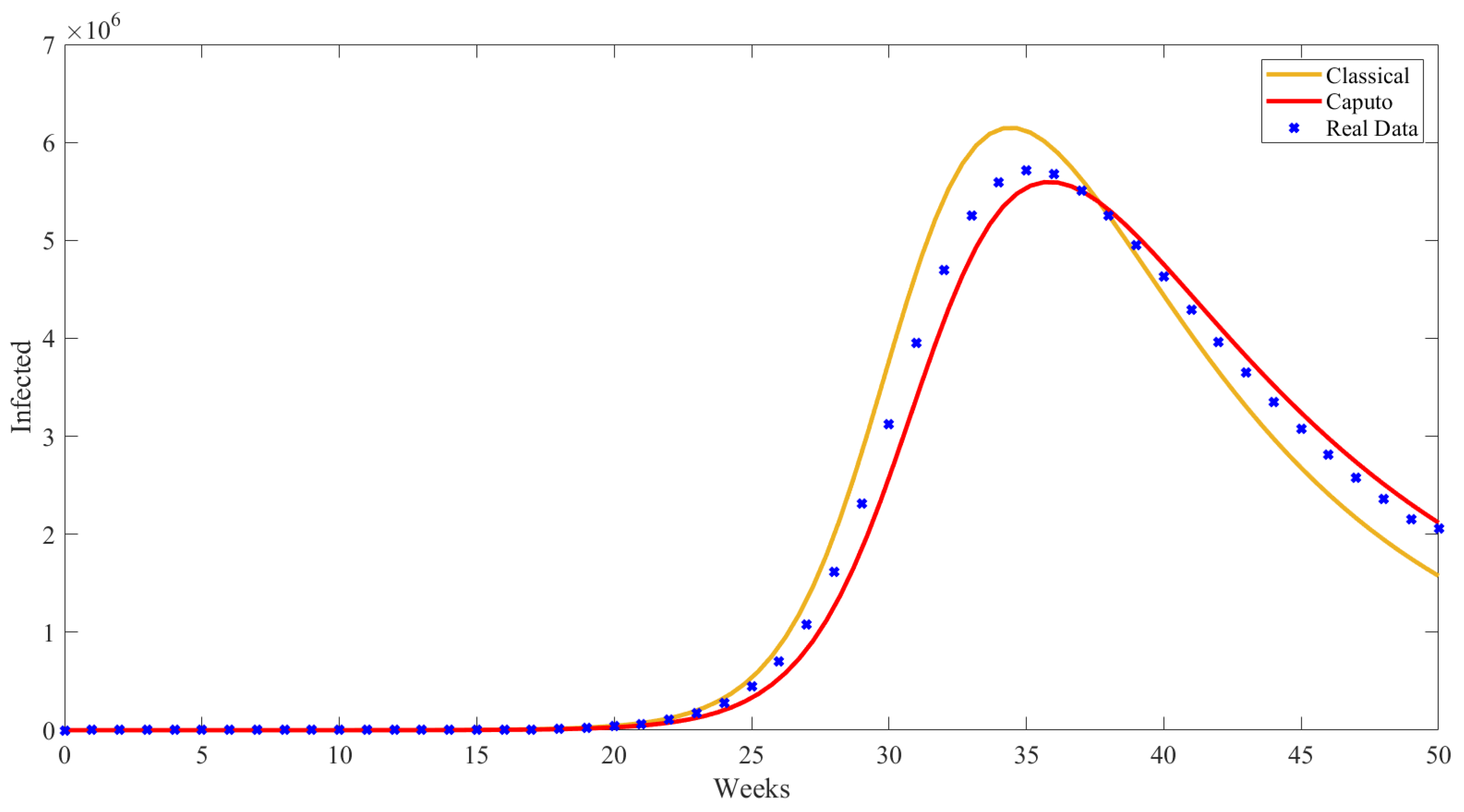
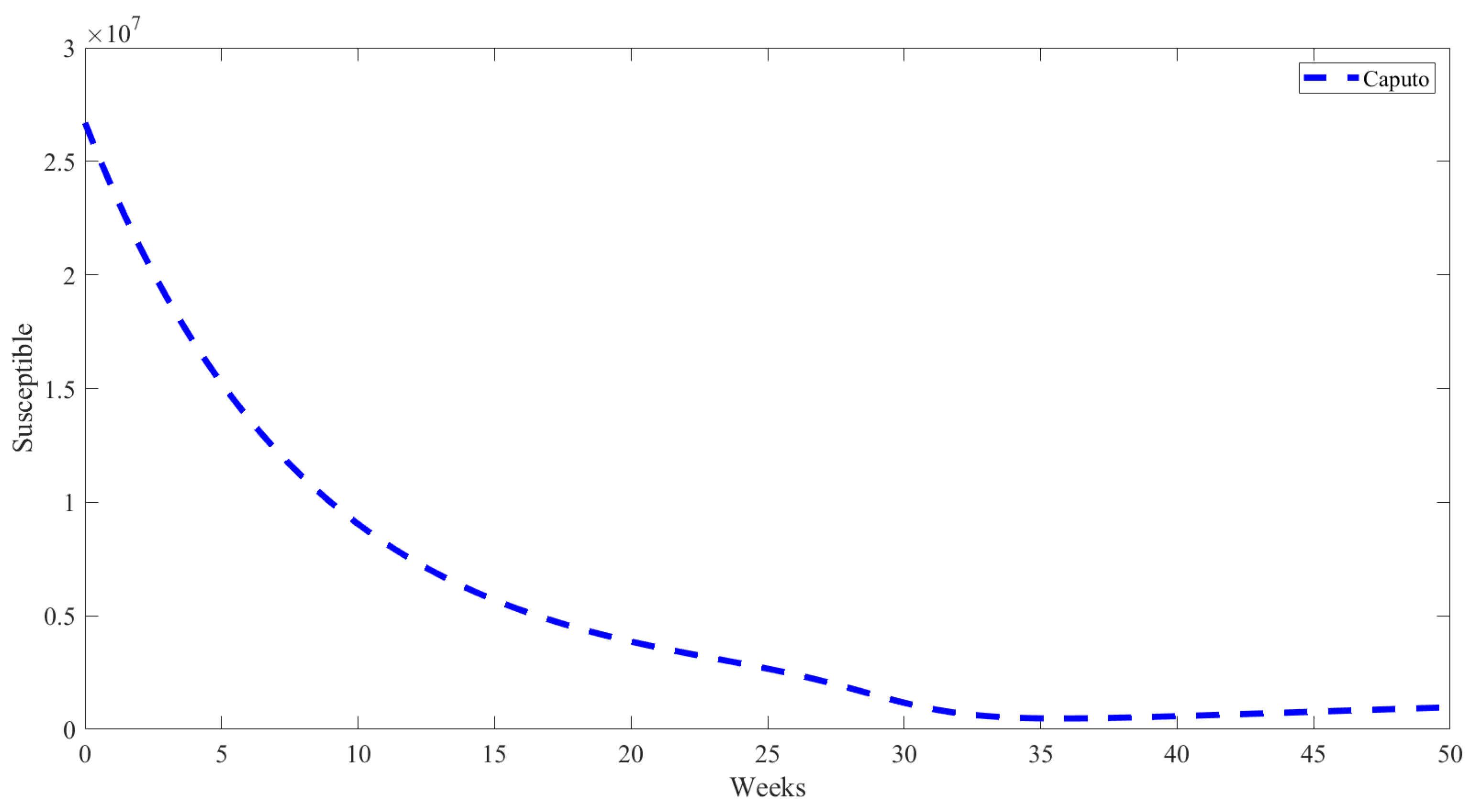
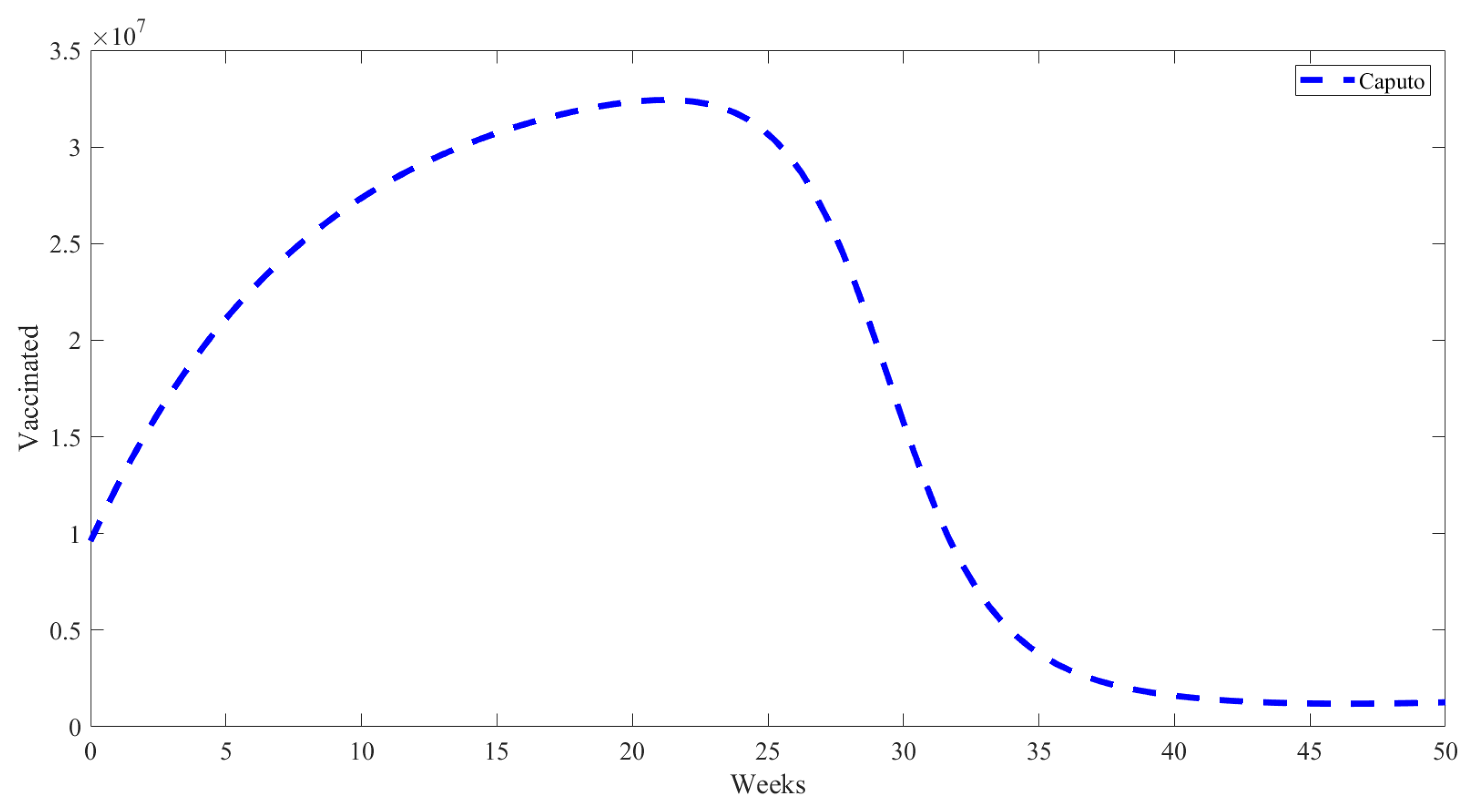
5. Numerical Results from Simulations

In this section, we find approximate solutions for the models (4) under Caputo fractional operators, using efficient numerical methods. Model summaries follow.

$${ }^{*}{\mathcal{D}}_{0,t}^{\alpha }g\left(t\right)=W\left(g\left(t\right)\right),t\in [0,a],g\left(0\right)=x_0,$$

(19)

where * is a fractional-order operator, and $x_0$ is the system’s starting state.

Using the fractional-order integral operators on Definition (1), one obtains

$$g\left(t\right)=x_0+I_{0,t}^{\alpha }W\left(g\left(t\right)\right),t\in [0,a],$$

(20)

Let $g_r$ approximate $g\left(t\right)$ at $t=t_r$ for $r=0,1,\dots ,n$ over $[0,a]$ with step length $\Delta t(=0.05)={\displaystyle \frac{a}{n}},n\in \mathbb{N}$. The scheme offers the following numerical methods for the underlying operators (see [33]).

$$C_{g_{r+1}}=x_0+{\displaystyle \frac{{(\Delta t)}^{\alpha }}{\mathsf{\Gamma }(\omega +1)}}\sum _{k=0}^r\left[{(r-k+1)}^{\omega }-{(r-k)}^{\omega }\right]W\left(g_k\right)+\mathcal{O}(\Delta t^2),$$

(21)

Figure 2 shows how the number of people infected changes over time. We used two mathematical models, the classical model and the Caputo derivative model, to predict the infection rates based on accurate data. The classical model predicted a rapid increase in infections starting around week 20, peaking at week 35. On the other hand, the Caputo derivative model anticipated slower growth and a gradual decline following the peak. The real data followed a similar pattern, with infections surging from around week 20 and reaching the highest point at week 35. The fractional Caputo derivative model more accurately represented the actual data, especially during the decline after the peak. The classical model overestimated the peak number of infections and did not capture the gradual deterioration observed in the data. This suggests that fractional models, like the fractional Caputo derivative model, may provide better forecasting accuracy when applied to accurate epidemic data.

The fractional Caputo derivative model was used to depict the temporal development of the susceptible population, as shown in Figure 3. The graph shows an initial sharp decline in the susceptible population, then a gradual slowdown over time. The curve is becoming less steep towards the end, suggesting that the model predicts a decrease in the number of individuals who are susceptible to the epidemic as it progresses, resulting in a more stable situation. The overall trend indicates that the fractional Caputo derivative model well captures the variations in the susceptible population as time progresses.

The dynamics of the vaccinated population over time are depicted in Figure 4 using the fractional Caputo derivative model. The figure illustrates a rapid initial increase in the population that has received vaccinations, followed by a consistent growth phase until the apex occurs around week 20. The vaccinated population experiences a substantial and swift decline following its apex. The vaccinated population is expected to stabilise towards the conclusion of the observation period, with the number of vaccinated individuals approaching zero, according to the fractional Caputo derivative model. This dynamic implies that the model takes into account factors such as the vaccination administration rate, the efficacy of the vaccination campaign, potential waning immunity, or other factors that may result in a decrease in the vaccinated population over time.

The Figure 5 shows how the number of people exposed to infection changes over several weeks using the fractional Caputo derivative model. In the beginning, only a few people are exposed, but around week 20, there is a significant increase. The highest number of people at risk of exposure is around weeks 27–28, usually during the winter. After that, the number of exposed people drops quickly and then levels off towards the end of the period. This pattern indicates a quick shift from a low-exposure period to a high one and then back to a low one, reflecting a short but intense period of exposure in the population.

Figure 6 illustrates the temporal evolution of the hospitalised individuals over time using the fractional Caputo derivative. It is clear from the graph that there are small numbers among the hospitalised population, and then the numbers begin to increase significantly starting from week 20. The number of patients requiring hospitalisation constantly increases, reaching its peak around week 35. After reaching its peak, there is a sharp decrease in the number of people admitted to hospitals, indicating a decrease in severe cases needing hospitalization. This phenomenon suggests that the model effectively represents the increase and decrease in hospitalisations, with a prominent phase of high numbers followed by a rapid decrease, mirroring the progression of an epidemic wave.

Figure 7 illustrates the temporal evolution of persons who recover over time using the fractional Caputo derivative model. The graph illustrates an insufficient number of individuals recover initially, followed by a substantial rise beginning at around week 20. There is a significant and rapid increase in the number of individuals who recover, beginning in week 25 and persisting until around week 35. Following the 40th week, the number of recovered persons remain constant, reaching a plateau after the observation period. This phenomenon indicates that the model accurately represents the recovery process, with an initial phase of quick improvement followed by stability as the epidemic wave diminishes and the number of infected people decreases.

The impact of memory trace on the behaviour of each sub-population for various alpha values is seen in Figure 8. Each curve corresponds to a different memory parameter value: 1 (blue), 0.9 (red), 0.8 (yellow), and 0.7 (purple). Based on the information provided in Figure 8, it can be seen that for $\alpha$ = 1, the curve stays constant, indicating the absence of a memory effect with a value of zero. The memory effect was observed in numerical simulations when it began exhibiting fractional-order values. Therefore, it is essential to include fractional-order derivatives with a memory effect to achieve the most accurate mathematical modelling.

Moreover, there was a strong correlation between the highest values of each subpopulation within the systems and the memory effect. Specifically, Figure 8a–f depicts the memory trace of the infected population over time in a fractional model of seasonal influenza. The data on the infected population figure indicated that reducing memory parameters resulted in increased variability in the infected population over time. The diagram illustrates the impact of memory on the behaviour of the infected population in a seasonal influenza model. A firmer memory effect, shown by a lower value of $\alpha$, resulted in more pronounced fluctuations in the number of infected people over time.

6. Conclusions

This work showed the substantial benefits of integrating the Caputo fractional differential operator into epidemiological models. The optimisation of the fractional-order parameter $\alpha$ = 0.99 demonstrated that the model better fitted empirical infection data than typical integer-order models. The results indicated that the fractional-order model produced more minor absolute mean errors, adequately representing the intricacies of illness transmission and progression. The results highlighted the crucial significance of the Caputo operator in improving the accuracy and forecasting ability of epidemiological models, offering significant knowledge for public health plans and treatments. Our future research will investigate the effects of non-singular differential operators on the traditional SVEIHR framework. This work will enhance the model’s resilience and relevance, potentially revealing novel illness dynamics and management aspects. Moreover, expanding the model to include more intricate interactions and diverse illness characteristics could yield a more profound understanding of the dynamics of infectious diseases in many circumstances. This continuous research will enhance the construction of epidemiological models that are even more precise and dependable, ultimately assisting in the creation of successful public health policies and interventions. More research is needed to understand the optimal disease control methods and how vaccinations and medications affect the fractional model and others [34,35,36,37,38,39,40,41].

References

1. Saunders-Hastings, P.R.; Krewski, D. Reviewing the history of pandemic influenza: Understanding patterns of emergence and transmission. Pathogens 2016, 5, 66. [Google Scholar] [CrossRef] [PubMed]
2. Barclay, W.; Openshaw, P. The 1918 Influenza Pandemic: One hundred years of progress, but where now? Lancet Respir. Med. 2018, 6, 588–589. [Google Scholar] [CrossRef] [PubMed]
3. Moghadami, M. A Narrative Review of Influenza: A Seasonal and Pandemic Disease. Iran. J. Med. Sci. 2016, 42, 2–13. [Google Scholar]
4. Dunning, J.; Thwaites, R.; Openshaw, P. Seasonal and pandemic influenza: 100 years of progress, still much to learn. Mucosal Immunol. 2020, 13, 566–573. [Google Scholar] [CrossRef] [PubMed]
5. Monto, A.S.; Gravenstein, S.; Elliott, M.; Colopy, M.; Schweinle, J. Clinical Signs and Symptoms Predicting Influenza Infection. Arch. Intern. Med. 2000, 160, 3243–3247. [Google Scholar] [CrossRef] [PubMed]
6. Paules, C.; Subbarao, K. Influenza. Lancet 2017, 390, 697–708. [Google Scholar] [CrossRef] [PubMed]
7. Pleschka, S. Overview of influenza viruses. In Swine Influenza; Springer: Berlin/Heidelberg, Germany, 2012; pp. 1–20. [Google Scholar]
8. Statista. Saudi Arabia: Life Expectancy at Birth from 2011 to 2022. Available online: https://www.statista.com/statistics/262477/life-expectancy-at-birth-in-saudi-arabia/ (accessed on 27 May 2024).
9. Quirouette, C.; Younis, N.P.; Reddy, M.B.; Beauchemin, C.A.A. A mathematical model describing the localization and spread of influenza A virus infection within the human respiratory tract. PLoS Comput. Biol. 2020, 16, 1–29. [Google Scholar] [CrossRef]
10. Dobrovolny, H.M.; Reddy, M.B.; Kamal, M.A.; Rayner, C.R.; Beauchemin, C.A.A. Assessing mathematical models of influenza infections using features of the immune response. PLoS ONE 2013, 8, e57088. [Google Scholar] [CrossRef] [PubMed]
11. Boianelli, A.; Nguyen, V.K.; Ebensen, T.; Schulze, K.; Wilk, E.; Sharma, N.; Stegemann-Koniszewski, S.; Bruder, D.; Toapanta, F.R.; Guzmán, C.A.; et al. Modeling influenza virus infection: A roadmap for influenza research. Viruses 2015, 7, 5274–5304. [Google Scholar] [CrossRef]
12. Handel, A.; Liao, L.E.; Beauchemin, C.A. Progress and trends in mathematical modelling of influenza A virus infections. Curr. Opin. Syst. Biol. 2018, 12, 30–36. [Google Scholar] [CrossRef]
13. Rvachev, L.A.; Longini, I.M. A mathematical model for the global spread of influenza. Math. Biosci. 1985, 75, 3–22. [Google Scholar] [CrossRef]
14. Kanyiri, C.W.; Mark, K.; Luboobi, L. Mathematical Analysis of Influenza A Dynamics in the Emergence of Drug Resistance. Comput. Math. Methods Med. 2018, 2018, 2434560. [Google Scholar] [CrossRef]
15. Malek, A.; Hoque, A. Mathematical modeling of the infectious spread and outbreak dynamics of avian influenza with seasonality transmission for chicken farms. Comp. Immunol. Microbiol. Infect. Dis. 2024, 104, 102108. [Google Scholar] [CrossRef] [PubMed]
16. Chlif, S.; Aissi, W.; Bettaieb, J.; Kharroubi, G.; Nouira, M.; Yazidi, R.; El Moussi, A.; Maazaoui, L.; Slim, A.; Ben Salah, A.; et al. Modelling of seasonal influenza and estimation of the burden in Tunisia. EMHJ-East. Mediterr. Health J. 2016, 22, 459–466. [Google Scholar] [CrossRef]
17. Evirgen, F.; Uçar, S.; Evirgen, F.; Özdemir, N. Modelling Influenza A disease dynamics under Caputo-Fabrizio fractional derivative with distinct contact rates. Math. Model. Numer. Simul. Appl. 2023, 3, 58–73. [Google Scholar] [CrossRef]
18. Yavuz, M.; Bonyah, E. New approaches to the fractional dynamics of schistosomiasis disease model. Phys. A Stat. Mech. Its Appl. 2019, 525, 373–393. [Google Scholar] [CrossRef]
19. Farman, M.; Akgül, A.; Nisar, K.S.; Ahmad, D.; Ahmad, A.; Kamangar, S.; Saleel, C.A. Epidemiological analysis of fractional order COVID-19 model with Mittag-Leffler kernel. AIMS Math. 2022, 7, 756–783. [Google Scholar] [CrossRef]
20. Joshi, H.; Jha, B.K. Chaos of calcium diffusion in Parkinson’s infectious disease model and treatment mechanism via Hilfer fractional derivative. Math. Model. Numer. Simul. Appl. 2021, 1, 84–94. [Google Scholar] [CrossRef]
21. Bonyah, E.; Yavuz, M.; Baleanu, D.; Kumar, S. A robust study on the listeriosis disease by adopting fractal-fractional operators. Alex. Eng. J. 2022, 61, 2016–2028. [Google Scholar] [CrossRef]
22. Özköse, F.; Yavuz, M.; Şenel, M.T.; Habbireeh, R. Fractional order modelling of omicron SARS-CoV-2 variant containing heart attack effect using real data from the United Kingdom. Chaos Solitons Fractals 2022, 157, 111954. [Google Scholar] [CrossRef]
23. Ahmed, I.; Akgül, A.; Jarad, F.; Kumam, P.; Nonlaopon, K. A Caputo-Fabrizio fractional-order cholera model and its sensitivity analysis. Math. Model. Numer. Simul. Appl. 2023, 3, 170–187. [Google Scholar] [CrossRef]
24. Yavuz, M.; Özköse, F.; Susam, M.; Kalidass, M. A New Modeling of Fractional-Order and Sensitivity Analysis for Hepatitis-B Disease with Real Data. Fractal Fract. 2023, 7, 165. [Google Scholar] [CrossRef]
25. Özköse, F. Long-Term Side Effects: A Mathematical Modeling of COVID-19 and Stroke with Real Data. Fractal Fract. 2023, 7, 719. [Google Scholar] [CrossRef]
26. Tassaddiq, A.; Qureshi, S.; Soomro, A.; Abu Arqub, O.; Senol, M. Comparative analysis of classical and Caputo models for COVID-19 spread: Vaccination and stability assessment. Fixed Point Theory Algorithms Sci. Eng. 2024, 2024, 1–23. [Google Scholar] [CrossRef]
27. Podlubny, I. Fractional Differential Equations: An Introduction to Fractional Derivatives, Fractional Differential Equations, to Methods of Their Solution and Some of Their Applications; Elsevier: Amsterdam, The Netherlands, 1998. [Google Scholar]
28. Caputo, M. Linear Models of Dissipation whose Q is almost Frequency Independent-II. Geophys. J. R. Astron. Soc. 2007, 13, 529–539. [Google Scholar] [CrossRef]
29. Ma, W.; Ma, N.; Dai, C.; Chen, Y.; Wang, X. Fractional modeling and optimal control strategies for mutated COVID-19 pandemic. Math. Methods Appl. Sci. 2022. [Google Scholar] [CrossRef]
30. Cori, A.; Valleron, A.-J.; Carrat, F.; Tomba, G.S.; Thomas, G.; Boëlle, P.-Y. Estimating influenza latency and infectious period durations using viral excretion data. Epidemics 2012, 4, 132–138. [Google Scholar] [CrossRef] [PubMed]
31. Abdoon, M.A.; Saadeh, R.; Berir, M.; EL Guma, F.; Ali, M. Analysis, modeling and simulation of a fractional-order influenza model. Alex. Eng. J. 2023, 74, 231–240. [Google Scholar] [CrossRef]
32. den Driessche, P.V.; Watmough, J. Reproduction numbers and sub-threshold endemic equilibria for compartmental models of disease transmission. Math. Biosci. 2002, 180, 29–48. [Google Scholar] [CrossRef]
33. Qureshi, S.; Atangana, A. Mathematical analysis of dengue fever outbreak by novel fractional operators with field data. Phys. A Stat. Mech. Its Appl. 2019, 526, 121127. [Google Scholar] [CrossRef]
34. Ali, M.; Alzahrani, S.M.; Saadeh, R.; Abdoon, M.A.; Qazza, A.; Al-Kuleab, N.; EL Guma, F.; Ali, M.; Alzahrani, S.M.; Saadeh, R.; et al. Modeling COVID-19 spread and non-pharmaceutical interventions in South Africa: A stochastic approach. Sci. Afr. 2024, 24, e02155. [Google Scholar] [CrossRef]
35. Saadeh, R.; Abdoon, M.A.; Qazza, A.; Berir, M.; EL Guma, F.; Al-Kuleab, N.; Degoot, A.M. Mathematical modeling and stability analysis of the novel fractional model in the Caputo derivative operator: A case study. Heliyon 2024, 10, e26611. [Google Scholar] [CrossRef]
36. Abdulkream Alharbi, S.; A. Abdoon, M.; Saadeh, R.; Alsemiry, R.D.; Allogmany, R.; Berir, M.; EL Guma, F. Modeling and analysis of visceral leishmaniasis dynamics using fractional-order operators: A comparative study. Math. Methods Appl. Sci. 2024, 47, 9918–9937. [Google Scholar] [CrossRef]
37. EL Gumaa, F.; Abdoon, M.A.; Qazza, A.; Saadeh, R.; Arishi, M.A.; Degoot, A.M. Analyzing the Impact of Control Strategies on Visceral Leishmaniasis: A Mathematical Modeling Perspective. Eur. J. Pure Appl. Math. 2024, 17, 1213–1227. [Google Scholar] [CrossRef]
38. Alzahrani, S.M.; Saadeh, R.; Abdoon, M.A.; Qazza, A.; Guma, F.E.; Berir, M. Numerical simulation of an influenza epidemic: Prediction with fractional SEIR and the ARIMA model. Appl. Math. 2024, 18, 1–12. [Google Scholar]
39. Khan, M.S.; Ali, A.; Suhail, M.; Alotaibi, E.S.; Alsubaie, N.E. On the estimation of ridge penalty in linear regression: Simulation and application. Kuwait J. Sci. 2024, 51, 100273. [Google Scholar] [CrossRef]
40. Albishri, S.B.; Albednah, F.A.; Alenazi, N.S.; Alsubaie, N.E.; Elserafy, O.S. National assessment of emergency staff level of practice in the management of forensic evidence. Forensic Sci. Res. 2023, 8, 265–273. [Google Scholar] [CrossRef]
41. Alhuzaim, W.M.; Alojayri, A.M.; Albednah, F.A.; Alshehri, F.F.; Alomari, M.S.; Alyousef, M.A.; Alsubaie, N.E. Impact of work hours on the quality of life of adult employees with irritable bowel syndrome in Saudi Arabia. Cureus 2022, 14, e31983. [Google Scholar] [CrossRef]
Figure 1. Transmission dynamics of the fractional influenza model.
Symmetry 16 00929 g001
Figure 2. Comparing the classical model ( α = 1) to the Caputo model ( α = 0.99) using real data.
Symmetry 16 00929 g002
Figure 3. The dynamical behaviour of the susceptible individuals included in fractional model (4).
Symmetry 16 00929 g003
Figure 4. The dynamical behaviour of the vaccinated individuals included in fractional model (4).
Symmetry 16 00929 g004
Figure 5. The dynamical behaviour of the exposed individuals included in fractional model (4).
Symmetry 16 00929 g005
Figure 6. The dynamical behaviour of the hospitalized individuals included in fractional model (4).
Symmetry 16 00929 g006
Figure 7. The dynamical behaviour of the recovered individuals included in fractional model (4).
Symmetry 16 00929 g007
Figure 8. The effects of memory trace on each population of model (4). (a) S population, (b) V population, (c) E population, (d) I population, (e) H population, (f) R population.
Symmetry 16 00929 g008