
Spherical Superpixel Segmentation with Context Identity and Contour Intensity


Abstract
1. Introduction
- An efficient seed-sampling method is proposed by defining a neighborhood range and regional context identity, which could optimize both the quantity and distribution of seeds, leading to evenly distributing seeds across the panoramic surface.
- A subtle inter-pixel correlation measurement is put forward to enhance boundary adherence across different scales, thereby integrating the contour intensity to pixel-superpixel correlation measurements.
- A context identity and contour intensity strategy is introduced to enhance the overall performance within a non-iterative clustering framework. Extensive experiments on two datasets were conducted, confirming its feasibility and comparable results.
2. Preliminaries on SNIC
3. Method
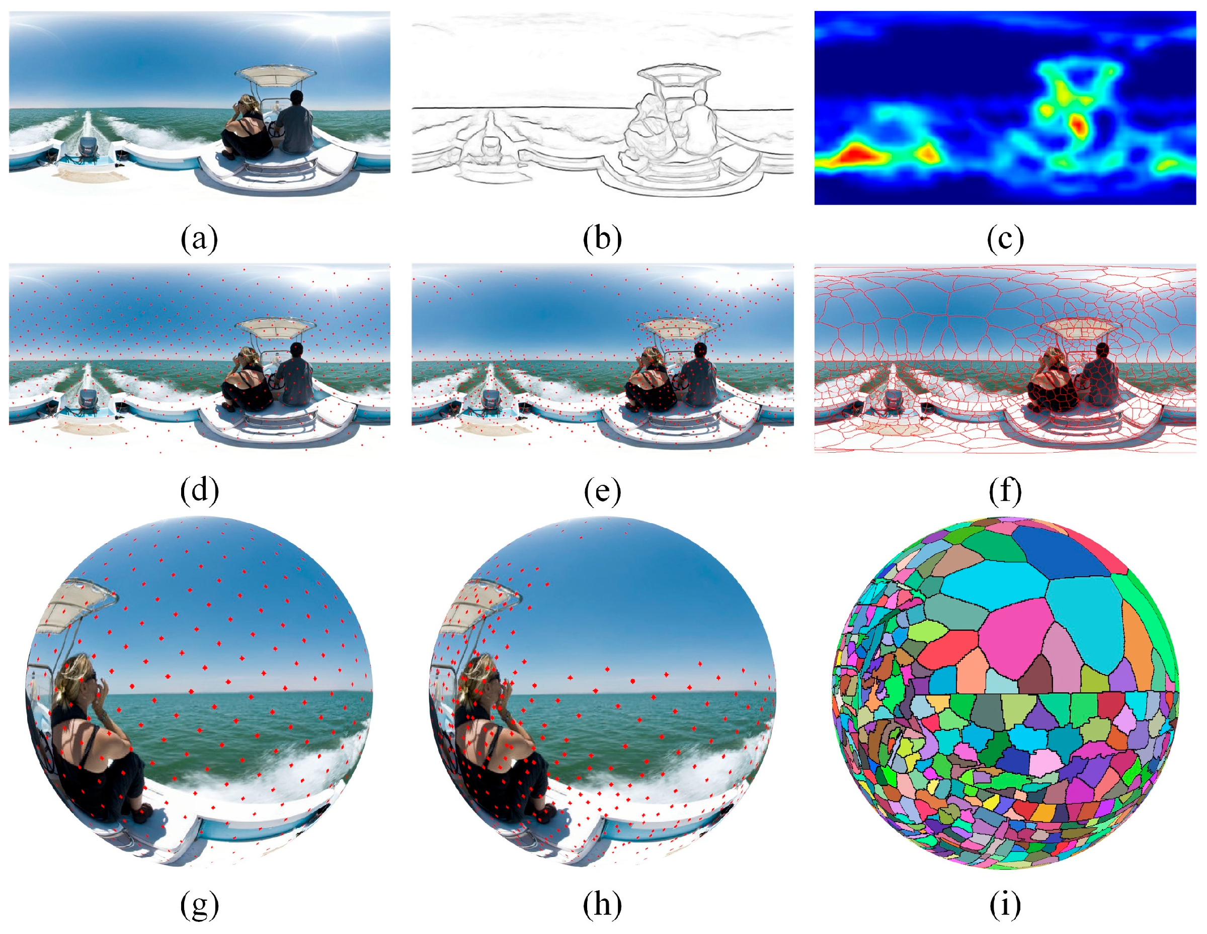
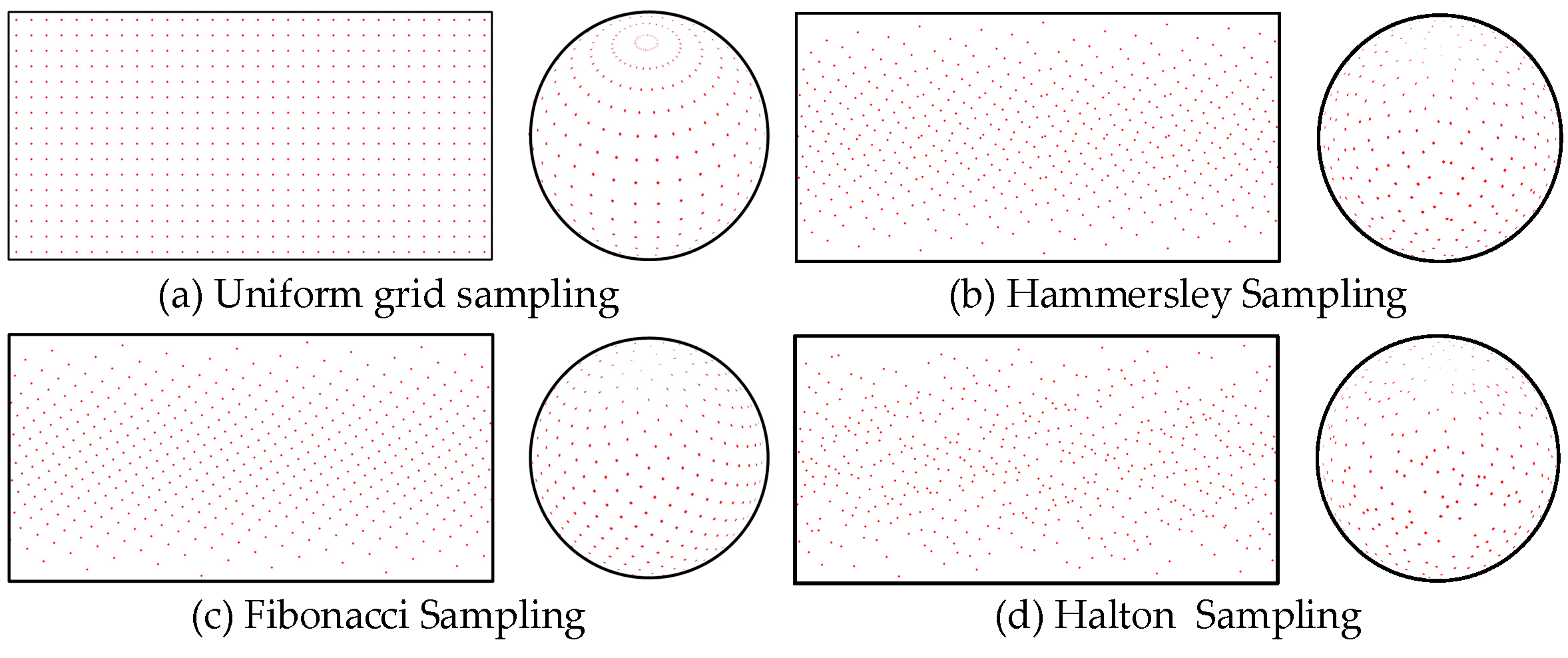
3.1. Sampling Strategies for Spherical Image
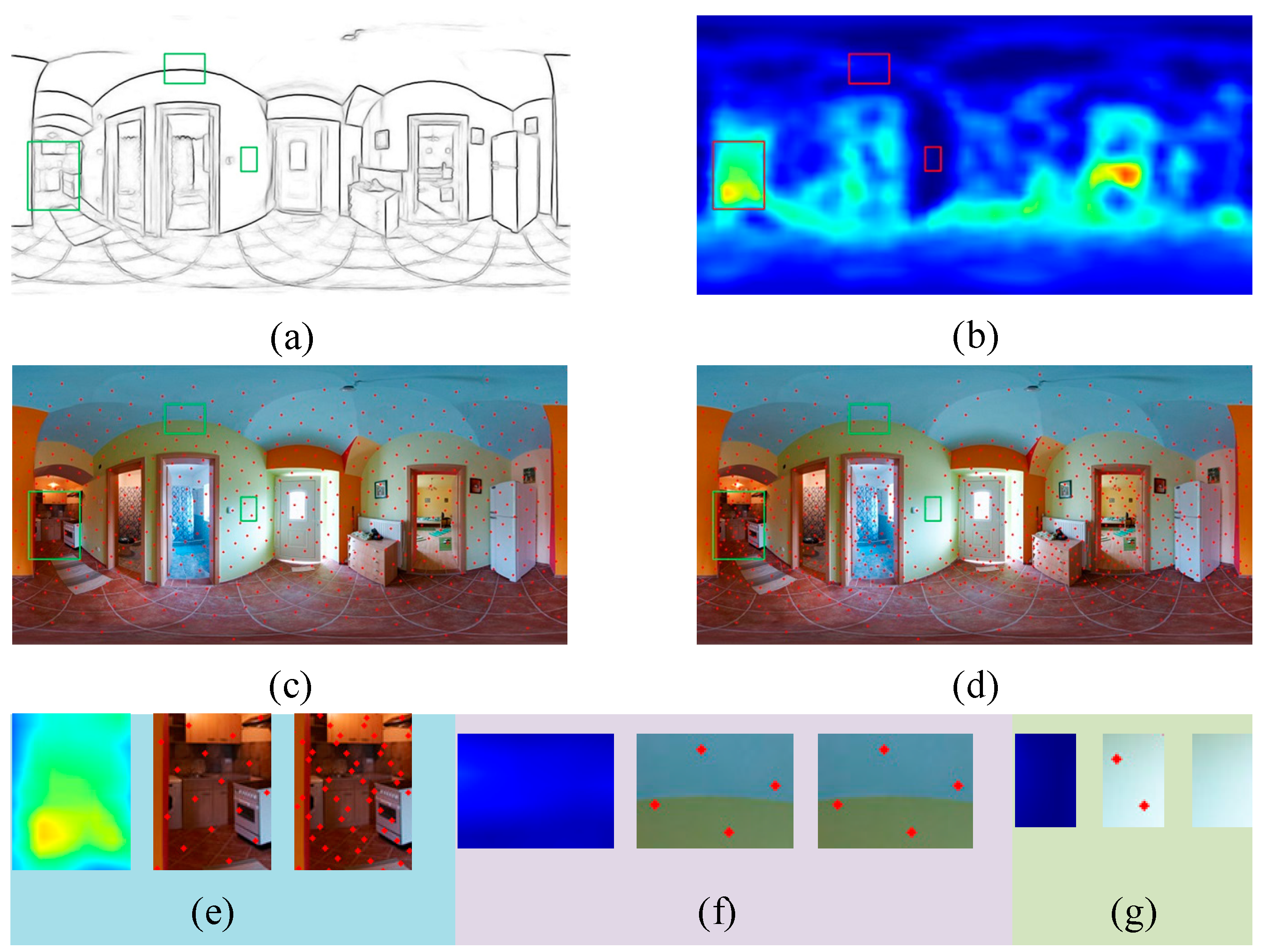
3.2. Optimized Initialization by Context Identity
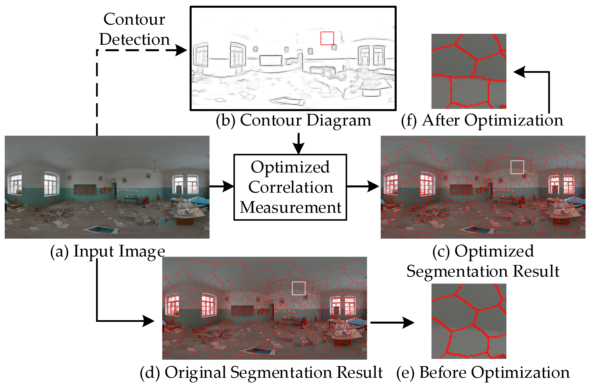
3.3. Optimized Correlation Measurement
- Distance measurement . The color component of pixel is . The color component of seed is , then is defined as follows:
- Spatial distance metric . The position mark of pixel on the spherical image is . Similarly, the coordinate of seed on the spherical image is . Therefore, is defined as follows:
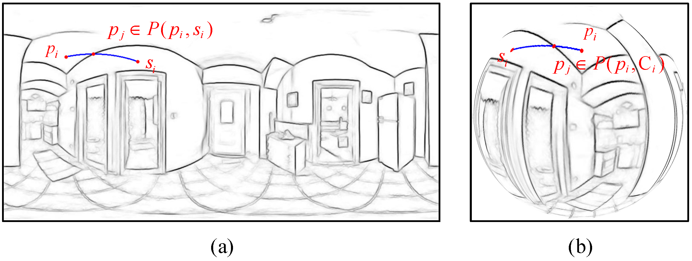
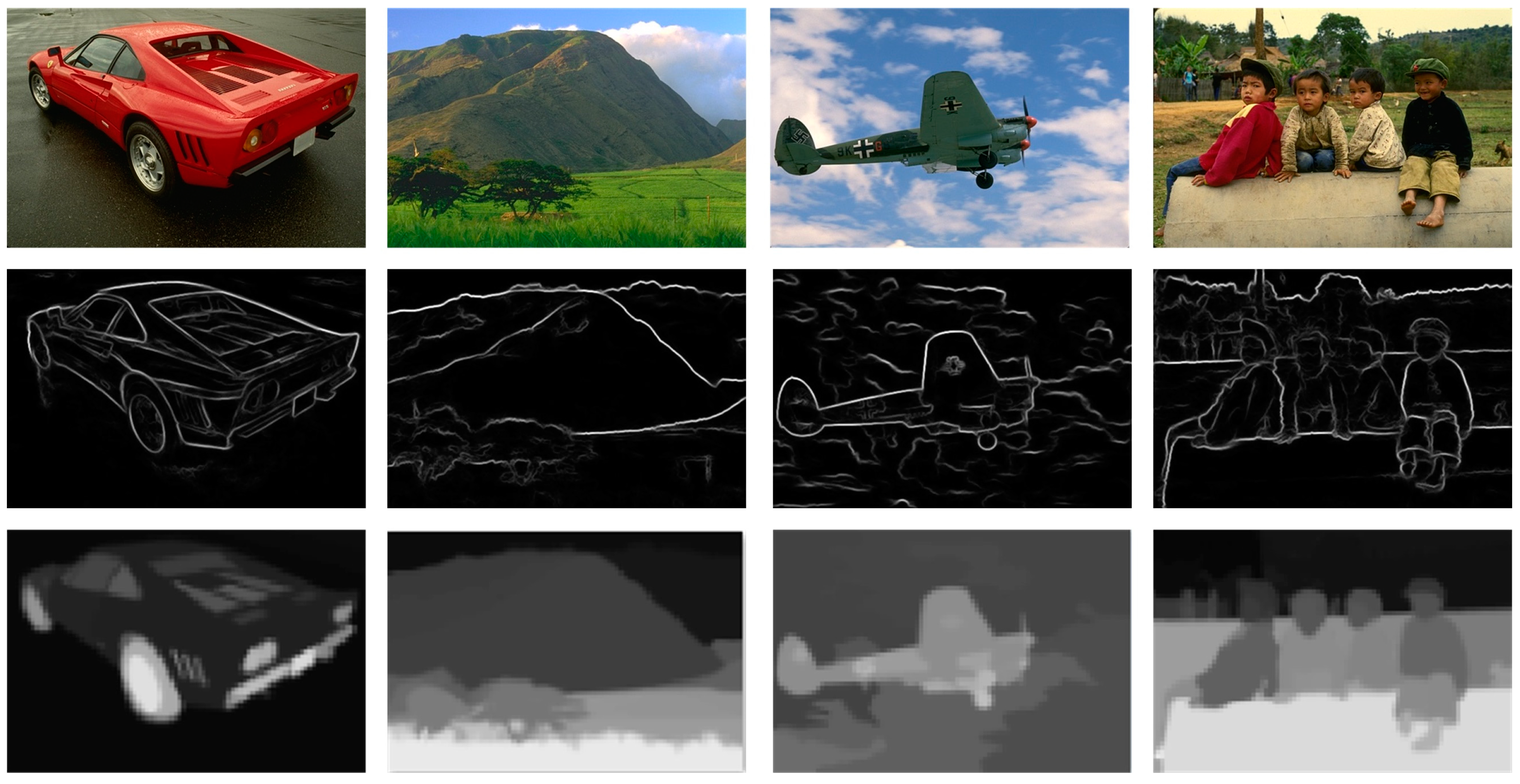
- Contour term component . The contour term is solved on the contour diagram of the original image. On the ERP image, traverse the shortest path between pixel in the contour map and seed , as shown in Figure 5. If the gray value of pixel on the shortest path is less than , . Then it means that there is a contour line between and . Therefore, is defined as follows:
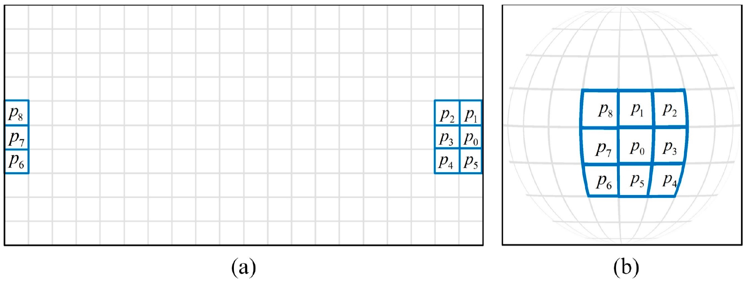
3.4. Boundary Neighborhood
| Algorithm 1: CICI spherical superpixel segmentation framework |
| Input: the EPR image , the contour map , the expected superpixel number |
| Output: Assigned label map |
| /*Initialization*/ |
| Initialize cluster seeds by Fibonacci sampling. Initialize a priority queue with a small root. Divided the area of each seed /*Seeds redistribution*/ for each region do Calculate the context identity of the current region . end for Calculate the context identity and the regional average context identity of Adjust the number of initial seeds to according to the context identity. Determine and . |
| for each region do if then Add two new seeds to area . else if then Keep the seeds in region unchanged. else if then Delete the seeds in area . end if |
| end for for do Create element through seeds and push in priority queue . end for /*label map update*/ |
| while is not empty do |
| Pop the element from queue . if is not labeled before then Assign the label to . Update the corresponding cluster. for traversing pixel new 8-neighborhood pixel do if is not labeled before then Update the distance and create the corresponding node . Push onto . |
| end if |
| end for end if end while |
| Return the label map . |
4. Experiments
4.1. SPSDataset75
4.1.1. Qualitative Result Analysis
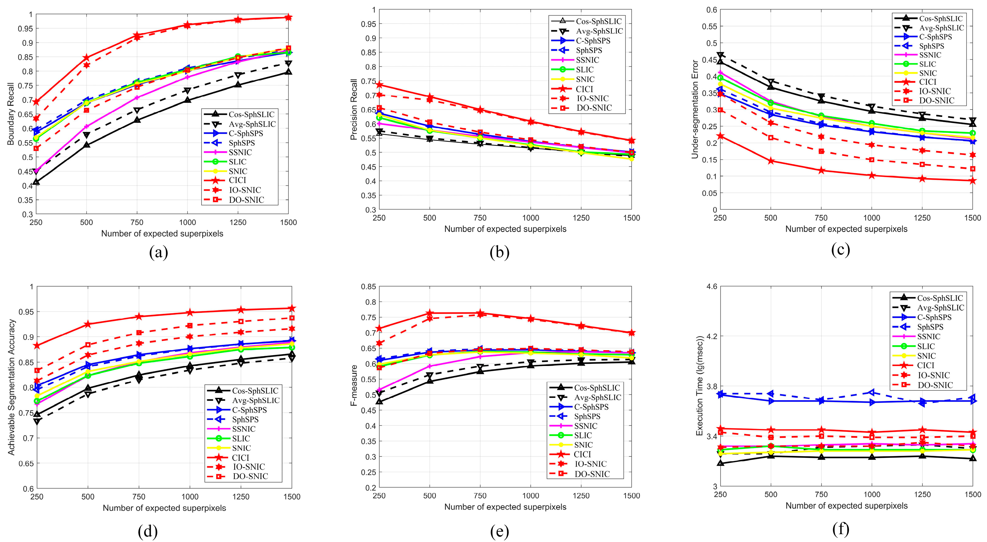
4.1.2. Quantitative Evaluation by Metrics
4.2. BSDS500
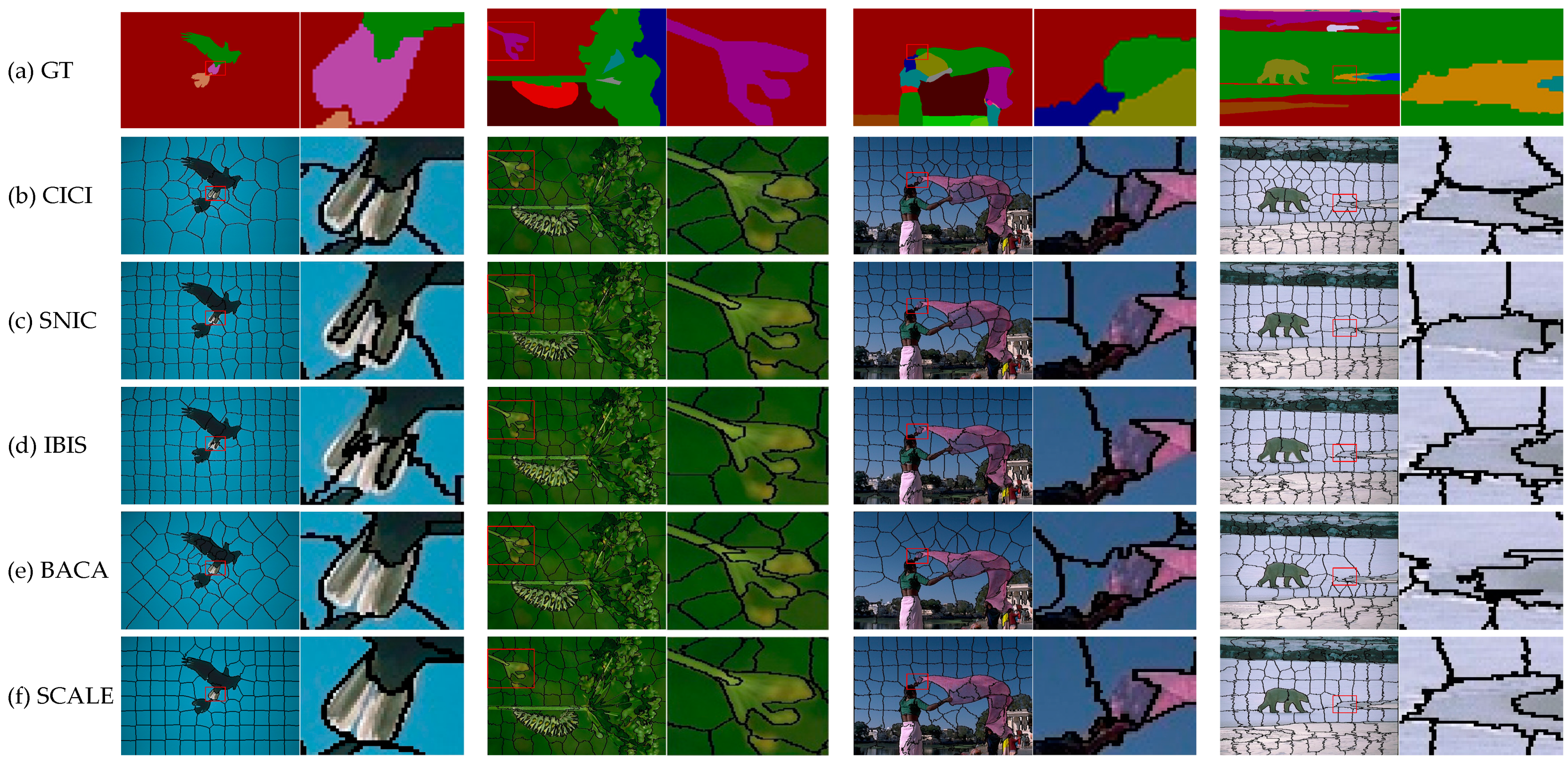
4.2.1. Qualitative Result Analysis
4.2.2. Quantitative Evaluation by Metrics
5. Conclusions
Author Contributions
Funding
Data Availability Statement
Acknowledgments
Conflicts of Interest
Appendix A

| Algorithm | Expected Superpixel Number | ||||||
|---|---|---|---|---|---|---|---|
| 250 | 500 | 750 | 1000 | 1250 | 1500 | ||
| BR | SLIC | 0.5637 | 0.6893 | 0.7607 | 0.8049 | 0.8510 | 0.8651 |
| SNIC | 0.5678 | 0.6887 | 0.7558 | 0.8003 | 0.8483 | 0.8792 | |
| SSNIC | 0.4512 | 0.6065 | 0.7072 | 0.7793 | 0.8324 | 0.8728 | |
| IO-SNIC | 0.6338 | 0.8207 | 0.9160 | 0.9585 | 0.9789 | 0.9878 | |
| DO-SNIC | 0.5297 | 0.6626 | 0.7443 | 0.8036 | 0.8468 | 0.8810 | |
| SphSPS | 0.5952 | 0.6983 | 0.7629 | 0.8102 | 0.8450 | 0.8728 | |
| C-SphSPS | 0.5863 | 0.6887 | 0.7526 | 0.8016 | 0.8362 | 0.8649 | |
| Cos-SphSLIC | 0.4108 | 0.5404 | 0.6277 | 0.6971 | 0.7509 | 0.7960 | |
| Avg-SphSLIC | 0.4513 | 0.5788 | 0.6651 | 0.7341 | 0.7878 | 0.8292 | |
| CICI | 0.6922 | 0.84677 | 0.9255 | 0.9621 | 0.9798 | 0.9877 | |
| PR | SLIC | 0.6211 | 0.5755 | 0.5505 | 0.5264 | 0.5008 | 0.4933 |
| SNIC | 0.6313 | 0.5771 | 0.5504 | 0.5242 | 0.4993 | 0.4766 | |
| SSNIC | 0.6008 | 0.5776 | 0.5556 | 0.5361 | 0.5167 | 0.4984 | |
| IO-SNIC | 0.7012 | 0.6825 | 0.6460 | 0.6064 | 0.5706 | 0.5408 | |
| DO-SNIC | 0.6563 | 0.6058 | 0.5704 | 0.5440 | 0.5199 | 0.4993 | |
| SphSPS | 0.6365 | 0.5914 | 0.5622 | 0.5373 | 0.5176 | 0.4996 | |
| C-SphSPS | 0.6365 | 0.5917 | 0.5626 | 0.5383 | 0.5174 | 0.5009 | |
| Cos-SphSLIC | 0.5645 | 0.5445 | 0.5283 | 0.5147 | 0.5012 | 0.4881 | |
| Avg-SphSLIC | 0.5747 | 0.5490 | 0.5327 | 0.5161 | 0.5006 | 0.4866 | |
| CICI | 0.7363 | 0.6945 | 0.6499 | 0.6087 | 0.5723 | 0.5418 | |
| UE | SLIC | 0.3951 | 0.3199 | 0.2808 | 0.2586 | 0.2356 | 0.2289 |
| SNIC | 0.3762 | 0.3044 | 0.2738 | 0.2503 | 0.2296 | 0.2155 | |
| SSNIC | 0.4109 | 0.3244 | 0.2794 | 0.2495 | 0.2294 | 0.2129 | |
| IO-SNIC | 0.3464 | 0.2599 | 0.2182 | 0.1937 | 0.1769 | 0.1639 | |
| DO-SNIC | 0.2987 | 0.2156 | 0.1745 | 0.1494 | 0.1351 | 0.1222 | |
| SphSPS | 0.3614 | 0.2919 | 0.2579 | 0.2346 | 0.2178 | 0.2057 | |
| C-SphSPS | 0.3472 | 0.2843 | 0.2532 | 0.2329 | 0.2173 | 0.2065 | |
| Cos-SphSLIC | 0.4422 | 0.3662 | 0.3247 | 0.2942 | 0.2726 | 0.2551 | |
| Avg-SphSLIC | 0.4649 | 0.3854 | 0.3412 | 0.3102 | 0.2865 | 0.2689 | |
| CICI | 0.2206 | 0.1458 | 0.1174 | 0.1022 | 0.0924 | 0.0863 | |
| ASA | SLIC | 0.7727 | 0.8233 | 0.8478 | 0.8612 | 0.8749 | 0.8790 |
| SNIC | 0.7832 | 0.8312 | 0.8512 | 0.8653 | 0.8779 | 0.8862 | |
| SSNIC | 0.7669 | 0.8230 | 0.8507 | 0.8680 | 0.8796 | 0.8889 | |
| IO-SNIC | 0.8131 | 0.8637 | 0.8870 | 0.9002 | 0.9091 | 0.9161 | |
| DO-SNIC | 0.8332 | 0.8843 | 0.9081 | 0.9221 | 0.9301 | 0.9372 | |
| SphSPS | 0.7952 | 0.8409 | 0.8618 | 0.8756 | 0.8854 | 0.8925 | |
| C-SphSPS | 0.8033 | 0.8449 | 0.8642 | 0.8766 | 0.8858 | 0.8919 | |
| Cos-SphSLIC | 0.7459 | 0.7979 | 0.8245 | 0.8426 | 0.8554 | 0.8657 | |
| Avg-SphSLIC | 0.7335 | 0.7872 | 0.8151 | 0.8339 | 0.8480 | 0.8580 | |
| CICI | 0.8828 | 0.9247 | 0.9399 | 0.9480 | 0.9531 | 0.9563 | |
| F-measure | SLIC | 0.5910 | 0.6272 | 0.6387 | 0.6365 | 0.6305 | 0.6283 |
| SNIC | 0.5978 | 0.6280 | 0.6369 | 0.6334 | 0.6285 | 0.6181 | |
| SSNIC | 0.5153 | 0.5916 | 0.6223 | 0.6352 | 0.6375 | 0.6344 | |
| IO-SNIC | 0.6657 | 0.7452 | 0.7577 | 0.7428 | 0.7209 | 0.6989 | |
| DO-SNIC | 0.5862 | 0.6329 | 0.6458 | 0.6488 | 0.6442 | 0.6373 | |
| SphSPS | 0.6151 | 0.6404 | 0.6474 | 0.6461 | 0.6420 | 0.6354 | |
| C-SphSPS | 0.6104 | 0.6365 | 0.6438 | 0.6441 | 0.6392 | 0.6343 | |
| Cos-SphSLIC | 0.4755 | 0.5424 | 0.5737 | 0.5921 | 0.6011 | 0.6051 | |
| Avg-SphSLIC | 0.5056 | 0.5639 | 0.5915 | 0.6061 | 0.6121 | 0.6132 | |
| CICI | 0.7135 | 0.7631 | 0.7636 | 0.7456 | 0.7225 | 0.6997 | |
| Execution Time (lg (ms)) | SLIC | 3.29 | 3.32 | 3.29 | 3.29 | 3.29 | 3.29 |
| SNIC | 3.26 | 3.27 | 3.28 | 3.28 | 3.28 | 3.29 | |
| SSNIC | 3.32 | 3.32 | 3.33 | 3.34 | 3.33 | 3.34 | |
| IO-SNIC | 3.31 | 3.32 | 3.32 | 3.32 | 3.35 | 3.32 | |
| DO-SNIC | 3.43 | 3.39 | 3.40 | 3.39 | 3.39 | 3.40 | |
| SphSPS | 3.74 | 3.74 | 3.69 | 3.75 | 3.66 | 3.71 | |
| C-SphSPS | 3.73 | 3.68 | 3.68 | 3.67 | 3.68 | 3.68 | |
| Cos-SphSLIC | 3.18 | 3.24 | 3.23 | 3.23 | 3.24 | 3.22 | |
| Avg-SphSLIC | 3.26 | 3.26 | 3.31 | 3.32 | 3.33 | 3.30 | |
| CICI | 3.46 | 3.45 | 3.45 | 3.43 | 3.45 | 3.43 | |
References
- Ren, X.; Malik, J. Learning a classification model for segmentation. In Proceedings of the Ninth IEEE International Conference on Computer Vision, Nice, France, 13–16 October 2003; pp. 10–17. [Google Scholar]
- Raine, S.; Marchant, R.; Kusy, B.; Maire, F.; Fischer, T. Point label aware superpixels for multi-species segmentation of underwater imagery. IEEE Robot. Autom. Lett. 2022, 7, 8291–9298. [Google Scholar] [CrossRef]
- Sheng, Y.; Ma, H.; Wang, X.; Hu, T.; Li, X.; Wang, Y. Weakly-supervised semantic segmentation with superpixel guided local and global consistency. Pattern Recognit. 2022, 124, 108504. [Google Scholar]
- Eliasof, M.; Zikri, N.B.; Treister, E. Unsupervised Image Semantic Segmentation through Superpixels and Graph Neural Networks. arXiv 2022, arXiv:2210.11810. [Google Scholar] [CrossRef]
- Zhou, Z.; Guo, Y.; Huang, J.; Dai, M.; Deng, M.; Yu, Q. Superpixel attention guided network for accurate and real-time salient object detection. Multimed. Tools Appl. 2022, 81, 38921–38944. [Google Scholar] [CrossRef]
- Lin, J.; Yan, Z.; Wang, S.; Chen, M.; Lin, H.; Qian, Z. Aerial image object detection based on superpixel-related patch. In Image and Graphics; Springer: Cham, Switzerland, 2021; Volume 12888, pp. 256–268. [Google Scholar]
- Xu, G.-C.; Lee, P.-J.; Bui, T.-A.; Chang, B.-H.; Lee, K.-M. Superpixel algorithm for objects tracking in satellite video. In Proceedings of the IEEE International Conference on Consumer Electronics-Taiwan (ICCE-TW), Penghu, Taiwan, 15–17 September 2021; pp. 1–2. [Google Scholar]
- Zhang, H.; Wang, H.; He, P. Correlation filter tracking based on superpixel and multifeature fusion. Optoelectron. Lett. 2021, 17, 47–52. [Google Scholar] [CrossRef]
- Nawaz, M.; Yan, H. Saliency detection via multiple-morphological and superpixel based fast fuzzy C-mean clustering network. Expert Syst. Appl. 2020, 16, 113654. [Google Scholar] [CrossRef]
- Nam, D.Y.; Han, J.K. Improved Depth Estimation Algorithm via Superpixel Segmentation and Graph-cut. In Proceedings of the IEEE International Conference on Consumer Electronics (ICCE), Las Vegas, NV, USA, 10–12 January 2021; pp. 1–7. [Google Scholar]
- Miao, Y.; Yang, B. Multilevel Reweighted Sparse Hyperspectral Unmixing Using Superpixel Segmentation and Particle Swarm Optimization. IEEE Geosci. Remote Sens. Lett. 2022, 19, 6013605. [Google Scholar] [CrossRef]
- Boulfelfel, S.; Nouboud, F. Multi-agent medical image segmentation: A survey. Comput. Methods Programs Biomed. 2023, 232, 107444. [Google Scholar]
- Sandler, M.; Zhmoginov, A.; Luo, L.; Mordvintsev, A.; Randazzo, E.; Arcas, B.A.Y. Image segmentation via cellular automata. arXiv 2020, arXiv:2008.04965. [Google Scholar]
- Zhao, Q.; Wan, L.; Zhang, J. Spherical superpixel segmentation. IEEE Trans. Multimed. 2017, 20, 1406–1417. [Google Scholar] [CrossRef]
- Wong, T.T.; Luk, W.S.; Heng, P.A. Sampling with Hammersley and Halton points. J. Graph. Tools 2012, 2, 9–24. [Google Scholar] [CrossRef]
- Wan, L.; Xu, X.; Zhao, Q.; Feng, W. Spherical Superpixels: Benchmark and Evaluation. In Computer Vision—ACCV 2018; Springer: Cham, Switzerland, 2018; Volume 11366, pp. 703–717. [Google Scholar]
- Giraud, R.; Pinheiro, R.B.; Berthoumieu, Y. Generalized shortest path-based superpixels for accurate segmentation of spherical images. In Proceedings of the 2020 25th International Conference on Pattern Recognition (ICPR), Milan, Italy, 10–15 January 2021; pp. 2650–2656. [Google Scholar]
- Achanta, R.; Susstrunk, S. Superpixels and polygons using simple non-iterative clustering. In Proceedings of the IEEE Con-ference on Computer Vision and Pattern Recognition (CVPR), Honolulu, HI, USA, 21–26 July 2017; pp. 4895–4904. [Google Scholar]
- Wei, X.; Yang, Q.; Gong, Y.; Ahuja, N.; Yang, M.H. Superpixel hierarchy. IEEE Trans. Image Process. 2018, 27, 4838–4849. [Google Scholar] [CrossRef]
- Silveira, D.; Oliveira, A.; Walter, M.; Jung, C.R. Fast and accurate superpixel algorithms for 360 images. Signal Process. 2021, 189, 108277. [Google Scholar] [CrossRef]
- Yuan, M.; Richardt, C. 360° optical flow using tangent images. arXiv 2021, arXiv:2112.14331. [Google Scholar]
- Huang, M.; Liu, Z.; Li, G.; Zhou, X.; Meur, O.L. FANet: Features Adaptation Network for 360° Omnidirectional Salient Object Detection. IEEE Signal Process. Lett. 2020, 27, 1819–1823. [Google Scholar] [CrossRef]
- Achanta, R.; Shaji, A.; Smith, K.; Lucchi, A.; Fua, P.; Süsstrunk, S. SLIC Superpixels Compared to State-of-the-Art Superpixel Methods. IEEE Trans. Pattern Anal. Mach. Intell. 2012, 34, 2274–2282. [Google Scholar] [CrossRef]
- Cabral, R.; Furukawa, Y. Piecewise Planar and Compact Floorplan Reconstruction from Images. In Proceedings of the IEEE Conference on Computer Vision and Pattern Recognition, Columbus, OH, USA, 23–28 June 2014; pp. 628–635. [Google Scholar]
- Hao, M.; Zhou, M.; Jin, J.; Shi, W. An Advanced Superpixel-Based Markov Random Field Model for Unsupervised Change Detection. IEEE Geosci. Remote Sens. Lett. 2019, 17, 1401–1405. [Google Scholar] [CrossRef]
- Dollar, P.; Zitnick, C.L. Structured forests for fast edge detection. In Proceedings of the IEEE international conference on computer vision, Sydney, NSW, Australia, 1–8 December 2013; pp. 1841–1848. [Google Scholar]
- Frisch, D.; Hanebeck, U.D. Deterministic gaussian sampling with generalized fibonacci grids. In Proceedings of the IEEE 24th International Conference on Information Fusion (FUSION), Sun City, South Africa, 1–4 November 2021; pp. 1–8. [Google Scholar]
- Arbeláez, P.; Maire, M.; Fowlkes, C.; Malik, J. Contour Detection and Hierarchical Image Segmentation. IEEE Trans. Pattern Anal. Mach. Intell. 2011, 33, 898–916. [Google Scholar] [CrossRef]
- Wang, M.; Liu, X.; Gao, Y.; Ma, X.; Soomro, N. Superpixel segmentation: A benchmark. Signal Process. Image Commun. 2017, 56, 28–39. [Google Scholar]
- Bobbia, S.; Macwan, R.; Benezeth, Y. Iterative Boundaries implicit Identification for superpixels Segmentation: A real-time approach. IEEE Access 2021, 9, 77250–77263. [Google Scholar] [CrossRef]
- Li, C.; He, W.; Liao, N.; Gong, J.; Hou, S.; Guo, B. Superpixels with contour adherence via label expansion for image decomposition. Neural Comput. Appl. 2022, 34, 16223–16237. [Google Scholar] [CrossRef]
- Liao, N.; Guo, B.; Li, C.; Liu, H.; Zhang, C. BACA: Superpixel segmentation with boundary awareness and content adaptation. Remote Sens. 2022, 14, 4572. [Google Scholar] [CrossRef]
- Van den Bergh, M.; Boix, X.; Roig, G.; Van Gool, L. SEEDS: Superpixels extracted via energy-driven sampling. Int. J. Comput. Vis. 2015, 111, 298–314. [Google Scholar] [CrossRef]
- Liu, M.; Tuzel, O.; Ramalingam, S.; Chellappa, R. Entropy rate superpixel segmentation. In Proceedings of the IEEE Confer-ence on Computer Vision and Pattern Recognition (CVPR), Colorado Springs, CO, USA, 20–25 June 2011; pp. 2097–2104. [Google Scholar]
- Chen, J.; Li, Z.; Huang, B. Linear spectral clustering superpixel. IEEE Trans. Image Process. 2017, 26, 3317–3330. [Google Scholar] [CrossRef]
- Zhao, J.; Hou, Q.; Ren, B.; Cheng, M.; Rosin, P. FLIC: Fast linear iterative clustering with active search. In Proceedings of the AAAI Conference on Artificial Intelligence (AAAI), New Orleans, LA, USA, 2–7 February 2018; pp. 7574–7581. [Google Scholar]


| Algorithm | Expected Superpixel Number | |||||||||
|---|---|---|---|---|---|---|---|---|---|---|
| 50 | 100 | 150 | 200 | 250 | 300 | 350 | 400 | 450 | 500 | |
| CICI | 0.7843 | 0.8592 | 0.8878 | 0.9008 | 0.9138 | 0.9229 | 0.9343 | 0.9366 | 0.9380 | 0.9442 |
| SNIC | 0.7069 | 0.8112 | 0.8561 | 0.8779 | 0.9038 | 0.9134 | 0.9221 | 0.9335 | 0.9415 | 0.9505 |
| IBIS | 0.6545 | 0.7622 | 0.7954 | 0.8408 | 0.8633 | 0.8755 | 0.8919 | 0.9139 | 0.9176 | 0.9286 |
| BACA | 0.9340 | 0.8153 | 0.8498 | 0.8659 | 0.8758 | 0.8818 | 0.8964 | 0.9071 | 0.9102 | 0.9155 |
| SCALE | 0.7183 | 0.8074 | 0.8489 | 0.8791 | 0.9000 | 0.9155 | 0.9278 | 0.9380 | 0.9471 | 0.9532 |
| Algorithm | Expected Superpixel Number | |||||||||
|---|---|---|---|---|---|---|---|---|---|---|
| 50 | 100 | 150 | 200 | 250 | 300 | 350 | 400 | 450 | 500 | |
| CICI | 0.0720 | 0.0508 | 0.0420 | 0.0414 | 0.0391 | 0.0372 | 0.0355 | 0.0349 | 0.0344 | 0.0338 |
| SNIC | 0.1133 | 0.0707 | 0.0575 | 0.0517 | 0.0455 | 0.0432 | 0.0420 | 0.0401 | 0.0373 | 0.0360 |
| IBIS | 0.1377 | 0.0954 | 0.0819 | 0.0701 | 0.0640 | 0.0597 | 0.0553 | 0.0513 | 0.0499 | 0.0473 |
| BACA | 0.0853 | 0.0578 | 0.0475 | 0.0458 | 0.0430 | 0.0403 | 0.0394 | 0.0384 | 0.0382 | 0.0369 |
| SCALE | 0.1294 | 0.0897 | 0.0755 | 0.0667 | 0.0600 | 0.0579 | 0.0547 | 0.0537 | 0.0512 | 0.0500 |
| Algorithm | Expected Superpixel Number | |||||||||
|---|---|---|---|---|---|---|---|---|---|---|
| 50 | 100 | 150 | 200 | 250 | 300 | 350 | 400 | 450 | 500 | |
| CICI | 0.9040 | 0.9317 | 0.9411 | 0.9442 | 0.9477 | 0.9499 | 0.9527 | 0.9539 | 0.9545 | 0.9558 |
| SNIC | 0.8677 | 0.9140 | 0.9293 | 0.9351 | 0.9425 | 0.9448 | 0.9476 | 0.9496 | 0.9525 | 0.9543 |
| IBIS | 0.8578 | 0.9004 | 0.9118 | 0.9234 | 0.9297 | 0.9337 | 0.9378 | 0.9424 | 0.9439 | 0.9462 |
| BACA | 0.8788 | 0.9113 | 0.9268 | 0.9313 | 0.9360 | 0.9380 | 0.9428 | 0.9456 | 0.9460 | 0.9477 |
| SCALE | 0.8730 | 0.9092 | 0.9227 | 0.9307 | 0.9350 | 0.9405 | 0.9434 | 0.9453 | 0.9476 | 0.9489 |
| Algorithm | Expected Superpixel Number | |||||||||
|---|---|---|---|---|---|---|---|---|---|---|
| 50 | 100 | 150 | 200 | 250 | 300 | 350 | 400 | 450 | 500 | |
| CICI | 0.4002 | 0.4907 | 0.5569 | 0.5796 | 0.5849 | 0.5920 | 0.6496 | 0.7095 | 0.7196 | 0.7295 |
| SNIC | 0.3486 | 0.4321 | 0.4819 | 0.5046 | 0.5434 | 0.5536 | 0.5700 | 0.5920 | 0.6039 | 0.6233 |
| IBIS | 0.3315 | 0.3996 | 0.4365 | 0.4735 | 0.5008 | 0.5211 | 0.5332 | 0.5572 | 0.5691 | 0.5818 |
| BACA | 0.3917 | 0.4805 | 0.5429 | 0.5673 | 0.5753 | 0.5833 | 0.6357 | 0.6887 | 0.6983 | 0.7090 |
| SCALE | 0.3845 | 0.4313 | 0.4624 | 0.4859 | 0.5000 | 0.5228 | 0.5346 | 0.5486 | 0.5615 | 0.5717 |
| Algorithm | Expected Superpixel Number | |||||||||
|---|---|---|---|---|---|---|---|---|---|---|
| 50 | 100 | 150 | 200 | 250 | 300 | 350 | 400 | 450 | 500 | |
| CICI | 42 | 88 | 142 | 161 | 186 | 212 | 254 | 300 | 309 | 340 |
| SNIC | 40 | 96 | 150 | 187 | 260 | 294 | 330 | 400 | 442 | 504 |
| IBIS | 40 | 93 | 125 | 182 | 223 | 256 | 291 | 372 | 392 | 435 |
| BACA | 38 | 87 | 130 | 158 | 188 | 211 | 262 | 302 | 314 | 345 |
| SCALE | 50 | 100 | 150 | 200 | 250 | 300 | 350 | 400 | 450 | 500 |
Disclaimer/Publisher’s Note: The statements, opinions and data contained in all publications are solely those of the individual author(s) and contributor(s) and not of MDPI and/or the editor(s). MDPI and/or the editor(s) disclaim responsibility for any injury to people or property resulting from any ideas, methods, instructions or products referred to in the content. |
© 2024 by the authors. Licensee MDPI, Basel, Switzerland. This article is an open access article distributed under the terms and conditions of the Creative Commons Attribution (CC BY) license (https://creativecommons.org/licenses/by/4.0/).
Share and Cite
Liao, N.; Guo, B.; He, F.; Li, W.; Li, C.; Liu, H. Spherical Superpixel Segmentation with Context Identity and Contour Intensity. Symmetry 2024, 16, 925. https://doi.org/10.3390/sym16070925
Liao N, Guo B, He F, Li W, Li C, Liu H. Spherical Superpixel Segmentation with Context Identity and Contour Intensity. Symmetry. 2024; 16(7):925. https://doi.org/10.3390/sym16070925
Chicago/Turabian StyleLiao, Nannan, Baolong Guo, Fangliang He, Wenxing Li, Cheng Li, and Hui Liu. 2024. "Spherical Superpixel Segmentation with Context Identity and Contour Intensity" Symmetry 16, no. 7: 925. https://doi.org/10.3390/sym16070925
APA StyleLiao, N., Guo, B., He, F., Li, W., Li, C., & Liu, H. (2024). Spherical Superpixel Segmentation with Context Identity and Contour Intensity. Symmetry, 16(7), 925. https://doi.org/10.3390/sym16070925