1. Introduction
The study of calculus without the notion of limits is known as quantum calculus or
q-calculus. Historically, Euler (in the eighteenth century) obtained some basic formulae in
q-calculus. However, what is now known as
q-derivative and
q-integral was defined by Jackson [
1]. Quantum calculus has several applications in many areas, such as physics, quantum mechanics, analytic number theory, hypergeometric functions, theory of finite differences, gamma function theory, Bernoulli and Euler polynomials, combinatorics, multiple hypergeometric functions, Sobolev spaces, operator theory, geometric theory of analytic and harmonic univalent functions, Lie theory, particle physics, nonlinear electric circuit theory, mechanical engineering, theory of heat conduction, quantum mechanics, cosmology and statistics (see [
2,
3,
4,
5,
6,
7,
8]).
q-derivatives and
q-integrals were generalized in non-integer orders by Al-Salam [
9] and Agarwal [
10]. For more details in quantum calculus, we refer to the monograph [
11], and for some recent results, we refer to the papers [
12,
13,
14,
15,
16,
17,
18,
19] and references cited therein. The notion of quantum calculus on finite intervals was introduced by Tariboon and Ntouyas in [
20]. For some recent results of quantum calculus on finite intervals we refer to [
21].
Recently, in [
22], the definitions of the quantum derivative and quantum integral on finite intervals were introduced with respect to another function and their basic properties were studied. The new theory of quantum calculus was applied and a new Hermite–Hadamard inequality for a convex function was obtained in addition to an existence and uniqueness result for an impulsive boundary value problem involving the quantum derivative with respect to another function.
In this research, we advance one step further in the study of quantum calculus on finite intervals with respect to another function of [
22], by studying a quantum coupled impulsive system with respect to another function of the form
where
are strictly increasing functions on
are fixed points in
are the nonlinear functions;
, and are the sequences of real numbers;
, and are the real constants.
We establish existence and uniqueness results by applying Banach fixed-point theorem and Leray–Schauder alternative. Our results are new and they enrich the literature to this new subject on quantum calculus on finite intervals with respect to another function. The used method is standard, but its configuration on quantum coupled impulsive systems with respect to another function is new.
This paper is organized as follows: In
Section 2, we recall the new results on quantum calculus on finite intervals with respect to another function. A basic lemma concerning a linear valiant of the problem (1) is also proved. In
Section 3, we study a quantum coupled impulsive system with respect to another function. The obtained results are well illustrated by numerical examples.
2. Preliminaries
Let a strictly increasing function and q be a quantum number with . Let us present the new definition of quantum derivative with respect to the function .
Definition 1 ([
22]).
Let be a continuous function. Then, the q-derivative of s with respect to ψ, on , is defined byand . Remark 1 ([
22]).
If , theni.e., we obtain the Tariboon–Ntouyas quantum derivative defined in [20]. For , we obtain the Jackson’s quantum derivative [1]: Example 1.
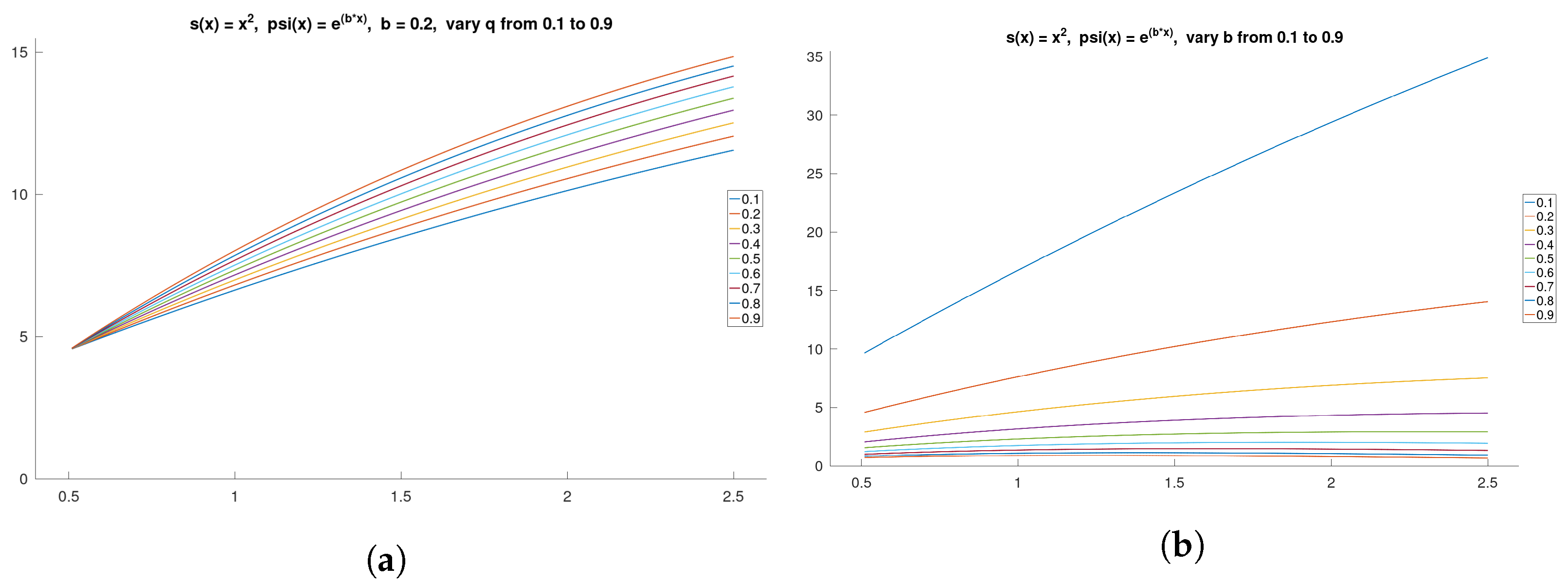
Let us consider an example for a computation of quantum derivative with respect to another function. Let , and , then By varying the parameters
q and
b, we illustrate their influence on the quantum derivative to a given function
.
Figure 1a shows the impact of the quantum parameter
q, varied from
to
, while we fixed parameter
b to
. Then, we fix the quantum number to
and vary parameter
b from
to
, with the results displayed in
Figure 1b. And the considered domain of this example is chosen to be
The graphs demonstrate that increasing the quantum number
q makes the curve slightly steeper, whereas increasing the parameter
b results in more significant changes to the graph, but in an opposite manner.
In the next lemma, we collect the basic properties of the quantum derivative with respect to another function.
Lemma 1 ([
22]).
We have the following:- (i)
- (ii)
- (iii)
where for all .
Now, we define the quantum integral with respect to another function.
Definition 2 ([
22]).
The definite quantum integral of with respect to function ψ and quantum number q, is defined by which is well defined if the right-hand side exists. Moreover, for , the definite quantum integral can be written as Remark 2 ([
22]).
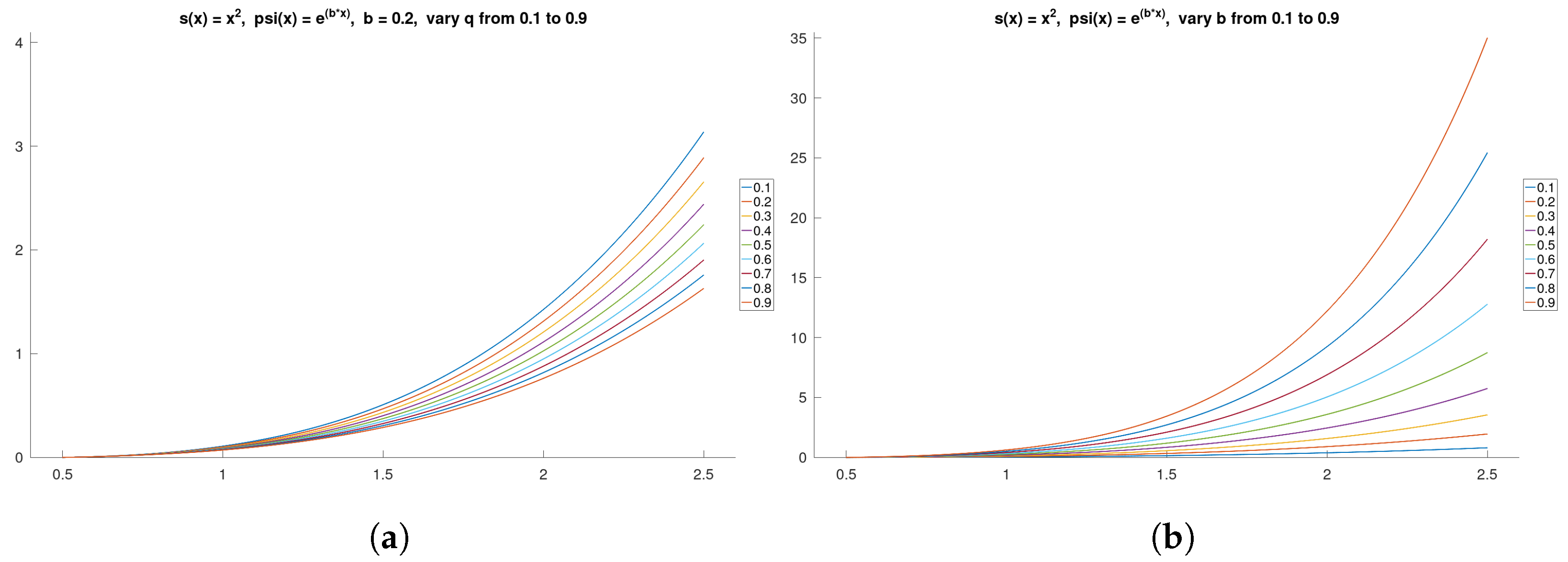
If , theni.e., we have the Tariboon–Ntouyas [20] definite quantum integral; and if , we have the Jackson [1] definite quantum integral: Example 2. Let us consider an example for the computation of the definite quantum integral with respect to another function. Let , and , then We investigate the impact of the quantum number
q and parameter
b on the definite quantum integral by varying these parameters. In
Figure 2a, parameter
b is set to
while the quantum number
q is adjusted from
to
. Conversely, in
Figure 2b, the quantum number
q is fixed at
, and parameter
b is varied from
to
. The selected domain remains
. To visualize the result, we approximate the definite integral, which is expressed as an infinite sum, by setting
. The results indicate that increasing parameter
b significantly sharpens the curve, whereas increasing the quantum number
q slightly reduces its steepness. The observed pattern exhibits an opposite trend compared to the quantum derivative example.
The following lemma concerns a linear variant of the initial system (
1) and is the basic tool to transform the nonlinear coupled impulsive quantum system (
1) into a fixed-point problem.
Lemma 2. Let and Then, satisfies the linear systemif and only ifandwhere Proof. For
, taking the operator
to both sides in the first equation in (4), we have
For
, taking the operator
to both sides in the first equation in (4), we have
From conditions
, we obtain
Once again, for
, we obtain
Repeating the above process, for
, we have
Indeed, (8) is true for
by (7) using
and
, when
. For
, we have
which shows that (
8) is satisfied for
By mathematical induction, (8) holds for every
.
In a similar way, we can obtain
In particular, for
, we have
Substituting the values of
and
in the boundary conditions
and
and solving the resulting system, we find
and
Substituting and in Equations (8) and (9), we obtain the solutions (5) and (6). We can prove the converse by direct computation. □
3. Main Results
The space of piecewise continuous functions is defined as is continuous everywhere except for some such that and exist and for all . is a Banach space with norm The product space is a Banach space with norm
In view of Lemma 2, we define an operator
by
where
and
For convenience, the following notations are used:
Theorem 1. Assume the following:
There exists positive constants such that for all and
Ifthen the impulsive quantum coupled system (1) has a unique solution. Proof. Define
with
satisfying
where
and
. Applying condition
, we obtain
In the same way, we obtain
In the first step, we will show that
For any
, we have
Therefore,
. In the next step, we will show that the operator
is a contraction. Let
and
Then, we have
It follows from (13) and (14) that
Since
,
is a contraction operator. Consequently, applying Banach’s fixed-point theorem, a unique fixed point of operator
is obtained, which implies that the impulsive quantum coupled system (
1) has a unique solution. The proof is completed. □
The next existence result is based on the Leray–Schauder alternative [
23].
Theorem 2. Let be continuous functions satisfying
There exists for and such that for any , we have
If and , where for are defined in (11), then the impulsive quantum coupled system (1) has at least one solution on . Proof. For the operator
, it can be seen that
is continuous from the fact that the functions
are continuous. Next, consider a bounded subset
of
Note that for
,
We will show that
is uniformly bounded. For
, we obtain
which implies that
Consequently,
and thus,
is uniformly bounded.
Next, the equicontinuous property of operator
is proven. Let
for some
with
Then, we have
Therefore, the operator is equicontinuous, and thus, the operator is completely continuous.
Lastly, we will show that the set
is bounded. Let
, then
. For any
, we have
Consequently,
where
which proves that the set
is bounded. By the Leray–Schader alternative, the operator
has at least one fixed point. Hence, the impulsive quantum coupled system (
1) has at least one solution on
and this completes the proof. □
4. Examples
Example 3. Consider the following given coupled system of impulsive quantum difference equations with coupled boundary conditions: From (15), we can set a function and constants , , , , , , , , , , , , , , , With these parameters, we found , , , , , , , , .
For all
and
, we can check the Lipschitz condition (condition
in Theorem 1) of two given functions as
Choosing
and
leads us to compute that
which is the satisfied inequality in Theorem 1. Since all assumptions of Theorem 1 are fulfilled, we deduce that the boundary value problem of a coupled impulsive quantum system with respect to another function in (15) with
,
given by (18) and (19), respectively, has a unique solution on
.
Example 4. Consider the following coupled impulsive system via quantum difference with respect to another function with coupled boundary conditions: From the given system, we can choose a function and constants , , , , , , , , , , , , , , , Then, via Maple computing, we obtain , , , , , , , , .
From the given functions (21) and (22), for each
and
, the bounds can be considered as
By setting , , , , , , we obtain and . Application Theorem 2 tells us that a coupled impulsive system via quantum difference with respect to another function with coupled boundary conditions (20) with , given by (21) and (22), respectively, has at least one solution on an interval .
Example 5. Consider the following linear coupled impulsive system via quantum difference with respect to another function with coupled boundary conditions: Now, we set a function , , and constants , , , , , , , , , , , , , , , Then, via Maple computing, we obtain , , . From Lemma 2, we can obtain the unique solution of system (25) as shown in the graphs.
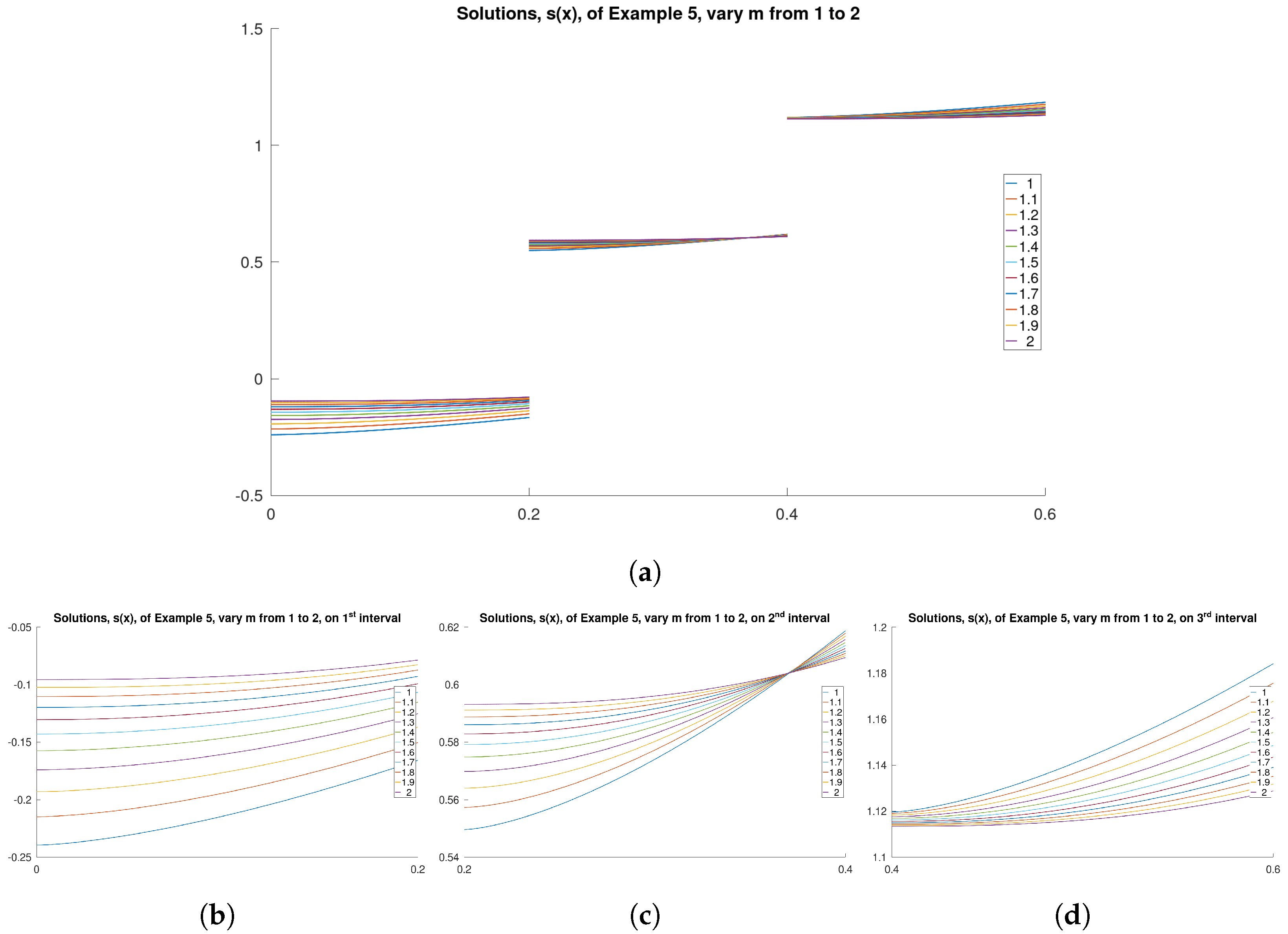
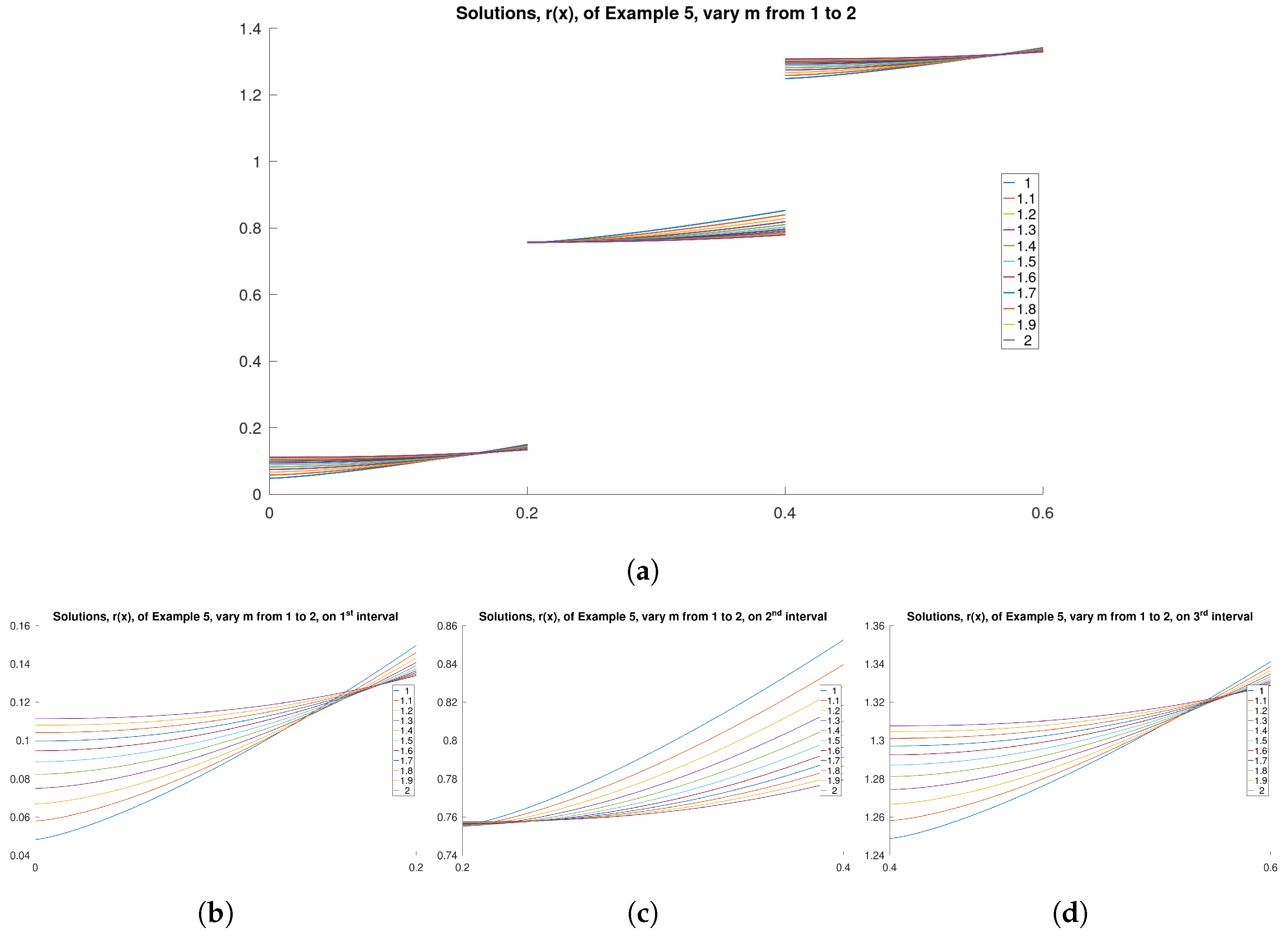
We visualize the numerical example by plotting the solutions of Example 5 to provide the reader with a clearer understanding of this work.
Figure 3 and
Figure 4 depict the solution functions,
s and
r, respectively, of this example by varying parameter
m from 1 to 2. The figures evidently demonstrate that functions
s and
r exhibit jump discontinuities as anticipated.
Figure 3a and
Figure 4a provide overviews of functions
s and
r across the entire considered domain, while
Figure 3b–d and
Figure 4b–d illustrate the values of functions
s and
r within each interval.


