Abundant Soliton Solutions to the Generalized Reaction Duffing Model and Their Applications

Abstract

The main aim of this study is to obtain soliton solutions of the generalized reaction Duffing model, which is a generalization for a collection of prominent models describing various key phenomena in science and engineering. The equation models the motion of a damped oscillator with a more complex potential than in basic harmonic motion. Two effective techniques, the mapping method and Bernoulli sub-ODE technique, are used for the first time to obtain the soliton solutions of the proposed model. Initially, the traveling wave transform, which comes from Lie symmetry infinitesimals, is applied, and a nonlinear ordinary differential equation form is derived. These approaches effectively retrieve a hyperbolic, Jacobi function as well as trigonometric solutions while the appropriate conditions are applied to the parameters. Numerous innovative solutions, including the kink wave, anti-kink wave, bell shape, anti-bell shape, W-shape, bright, dark and singular shape soliton solutions, were produced via the mapping and Bernoulli sub-ODE approaches. The research includes comprehensive 2D and 3D graphical representations of the solutions, facilitating a better understanding of their physical attributes and proving the effectiveness of the proposed methods in solving complex nonlinear equations. It is important to note that the proposed methods are competent, credible and interesting analytical tools for solving nonlinear partial differential equations.

1. Introduction

The majority of real-world occurrences are described by nonlinear evolution equations (NLEEs). Nonlinear processes are more difficult to deal with because of their nonlinear properties. Additionally, nonlinear processes are challenging to regulate since they can change quickly with only slight modifications to the basic parameters. Because of how complicated the issue is, a conclusive NLEE solution is needed. Numerous scientific and technical fields have benefited greatly from the precise traveling wave (TW) solutions to nonlinear partial differential equations (NLPDEs) [1]. These solutions have been important in the investigation of nonlinear physical processes including low-pressure wave propagation, chemical mechanics, geochemistry, computational physics, plasma physics, fluid mechanics, theory of quantum fields, biological physics and so forth. As is often known, a large number of NLEEs are employed to characterize these complex occurrences. Thus, a wide range of scientists are very interested in the effective and potent techniques for locating analytic solutions to nonlinear equations. A single combination of variables, such as TW variables, may be the only determinant of some of the potential solutions for special form NLEEs. In order to represent the propagation of powerful laser pulses through a nonlinear optical medium, complex soliton solutions are essential. They are employed in the description of phenomena like self-phase modulation and soliton self-focusing. For long-distance communication, solitons are used in fiber optics [2]. NLPDEs are a common exemplar of mathematical–physical systems; hence, the analytical solutions to these problems are critical. Many solid and direct methods have been developed for solving the NLPDEs, like the mapping method [3], exp-function method [4], sine–cosine technique [5], tanh–sech approach [6], modified extended tanh-function technique [7], extended F-expansion method [8], homogeneous balance technique [9], Jacobi elliptic function approach [10], modified simple equation technique [11], parameterized Adomian decomposition approach [12], modified exponential rational function approach [13], optimal homotopy asymptotic technique [14], modified trial equation approach [15], variational iterative technique [16], hyperbolic tangent function technique [17], Darboux transformation approach [18], extended FAN sub-equation strategy [19], Hirota’s bilinear scheme [20], auxiliary equation approach [21], tanh coth approach [22], Backlund transformation method [23], Riemann–Hilbert approach [24], residual power series technique [25], Fokas unified transform method [26], first integration method [27] and several others.

The nonlinear generalized reaction Duffing model (GRDM) is a highly significant mathematical model in physics. The equation exhibiting a cubic nonlinearity of an oscillator is known as the Duffing equation. George Duffing, a German engineer, authored a comprehensive book about this subject in 1918 [28]. The equation displays a wide range of well-known characteristics in nonlinear dynamical systems and is employed by numerous researchers to demonstrate this kind of behavior. Researchers into chaos have found it to be extremely popular since the 1970s, considering that it may be among the simplest equations describing a system’s chaotic behavior. Chaotic dynamics of the fractionally damped Duffing equation are discussed in [29]. In shallow areas above the flat seafloor, nonlinear equations like the GRDM show significant spectral energy transfer for finite amplitude waves. In mechanical systems, the Duffing equation can represent nonlinear vibrations, such as those occurring in mechanical structures subjected to external forces or excitations.

This study’s primary objective is to generate stable, widely applicable and compatible soliton solutions to the GRDM using the mapping method (MM) and the Bernoulli sub-ODE (BS-ODE) approach. It is evident how widely applicable the strategies are when applied to this equation. It is considered that the obtained results have not been established in prior studies via these methods, as the mapping and BS-ODE techniques have not been used to find the exact solution for the nonlinear GRDM. The exact solutions to the GRDM have been extracted for the first time using these methods. They offer a simple way to deal with solutions to NLPDEs. The mapping method [3] is used in this study to find the soliton and other solitary wave solutions of the GRDM. For the stochastic modified Korteweg–de Vries (KdV) equation, the mapping approach was applied in [30]. Rehman, et al. [31] obtained the optical solitons of the Biswas–Arshed model using the mapping approach. The novel mapping technique was used in [32] to obtain the solitons and other solutions for two nonlinear Schrödinger equations. In [33], soliton solutions of the (4 + 1)-dimensional Davey Stewartson Kadomtsev Petviashvili equation are derived using a modified extended mapping method. Because of their elastic dispersion characteristics, the solitary waves continue to maintain their speed and form even in collisions. Originally, the BS-ODE approach was intended to produce exact TW solutions, solitary wave solutions and peaked wave solutions for NLPDEs. In [34], NLPDEs were solved by the BS-ODE technique. The Riccati BS-ODE technique was used to solve some NLEEs in [35]. In [36], a novel BS-ODE technique was introduced for creating TW solutions for a pair of nonlinear equations of any order. The outcomes demonstrate that, compared to the other methods, the mapping and BS-ODE procedures are more accurate and need less processing resources. These findings have been applied to the field of mechanical engineering and have the potential to improve our comprehension of the range of phenomena that occur in the numerous physical systems that the current framework covers. These two approaches appear to be more practical, user-friendly and efficient based on the soliton analysis. Due to this, the goal of this work is to investigate the TW solutions of the GRDM utilizing the mapping method [37] and BS-ODE approach [38,39] emphasizing the effect of free parameter values on the obtained soliton solutions. Triki, et al. [40] obtained shock wave solutions to Bogoyavlensky-Konoplechenko equation using Ansatz approach.

The arrangement of this article is as follows: Section 2 presents the GRDM. The descriptions of the BS-ODE and mapping techniques are given in Section 3. In Section 4, the TW solutions of the GRDM are derived using the mapping method and the BS-ODE method. The graphical behaviors of TW solutions of the GRDM using the BS-ODE and mapping method are examined in Section 5. A comparison between the proposed and previous studies is discussed in Section 6. Section 7 presents the stability analysis of the proposed study. Some concluding remarks are listed in Section 8.

2. The Generalized Reaction Duffing Model

This section will describe the GRDM, which has the following form:

$${{\rm Y}}_{tt}+a{{\rm Y}}_{zz}+e{\rm Y}+g{{\rm Y}}^2+h{{\rm Y}}^3=0,t>0,$$

(1)

where $a,e,g$ and h are constants. If $g=0$, then Equation (1) converts into

$${{\rm Y}}_{tt}+a{{\rm Y}}_{zz}+e{\rm Y}+h{{\rm Y}}^3=0.$$

(2)

Consider the following wave transformation which comes from Lie symmetry infinitesimals $\frac{\partial }{\partial z}$ and $\frac{\partial }{\partial t}$ [41]

$$\varkappa =Bz-Kt,$$

(3)

where the constants B and K are non-zero.

3. Description of Analytical Approaches

The algorithm for using the mapping and BS-ODE approaches to obtain the exact solutions of the NLPDE is presented in this section. These techniques are described below as follows:

3.1. Mapping Method

The mapping method for deriving the TW solutions of NLEEs is explained in this section. Take into account the following NLPDE features two independent temporal and spatial variables,

$$R\left({\rm Y},{{\rm Y}}_t,{{\rm Y}}_z,{{\rm Y}}_{tt},{{\rm Y}}_{zz},{{\rm Y}}_{zt},\cdots \cdots \right)=0,$$

(4)

where ${\rm Y}\left(\varkappa \right)={\rm Y}\left(z,t\right)$ are unknown. ${\rm Y}\left(z,t\right)$ and its partial derivatives make up the polynomial R, comprising nonlinear terms and highest-order derivatives.

Step 1. The wave-transformation relation can be used to transform Equation (4) into the ordinary differential equation (ODE). The wave transformation is as follows:

$$\begin{array}{c}\hfill {\rm Y}\left(\varkappa \right)={\rm Y}\left(z,t\right),\\ \hfill \varkappa =Bz-Kt,\end{array}$$

(5)

where B and K are the wave number and velocity, respectively. Substituting Equation (5) into Equation (4) yields an ODE of ${\rm Y}\left(\varkappa \right)$

$$R({\rm Y},{{\rm Y}}^{\prime },{{\rm Y}}^{″},{{\rm Y}}^{‴},\cdots )=0,$$

(6)

where R is a polynomial in ${\rm Y}\left(\varkappa \right)$ with derivatives of ${\rm Y}\left(\varkappa \right)$ and prime represents the derivatives with respect to $\varkappa$ such that ${{\rm Y}}^{\prime }\left(\varkappa \right)=\frac{d{\rm Y}}{d\varkappa }$, ${{\rm Y}}^{″}\left(\varkappa \right)=\frac{{\mathrm{d}}^2{\rm Y}}{\mathrm{d}{\varkappa }^2}$ and so on.

If Equation (6) is integrable, then take each integral constant to be zero and integrate it as many times as needed.

Step 2. Assume that the formal solution of Equation (6) has the form

$${\rm Y}\left(\varkappa \right)=\sum _{i=0}^v{C}_i{m}^i\left(\varkappa \right),$$

(7)

where v is a positive integer that needs to be calculated and $C_i$ are real constants to be determined such that $C_v\ne 0$ is to be identified, while m satisfies the first kind of elliptic equation

$$\left\{\begin{array}{c}{m}^{″}=jm+k{m}^3,\hfill \\ m^{\prime 2}=j{m}^2+\frac{1}{2}k{m}^4+l.\hfill \end{array}\right.$$

(8)

Here, the prime means the derivative with respect to $\varkappa$.

Step 3. The number v is fixed by balancing the linear term of the highest-order derivative with a nonlinear term in Equation (5) and the power of nonlinearity in Equation (4).

Step 4. The coefficients $C_i,K,j,k$ and l can be found after substituting Equation (7) with (8) into the ODE in Equation (6). If one of them is left unspecified, it will be regarded as being arbitrary for the solution to Equation (4). Therefore, Equation (6) creates an algebraic mapping relation between Equations (4) and (7)’s solution.

Step 5. Equation (8) generate the following solutions,

$$\left\{\begin{array}{c}m\left(\varkappa \right)=tanh\left(\varkappa \right),\hfill \\ m\left(\varkappa \right)=sech\left(\varkappa \right),\hfill \\ m\left(\varkappa \right)=\mathrm{sn}\left(\varkappa \right),orm\left(\varkappa \right)=\mathrm{cd}\left(\varkappa \right),\hfill \\ m\left(\varkappa \right)=\mathrm{cn}\left(\varkappa \right),\hfill \\ m\left(\varkappa \right)=\mathrm{dn}\left(\varkappa \right),\hfill \\ m\left(\varkappa \right)=\mathrm{ns}\left(\varkappa \right),orm\left(\varkappa \right)=\mathrm{dc}\left(\varkappa \right),\hfill \end{array}\right.$$

(9)

where $\mathrm{sn}\left(\varkappa \right)$, $\mathrm{cn}\left(\varkappa \right)$, $\mathrm{dn}\left(\varkappa \right)$, $\mathrm{ns}\left(\varkappa \right)$, $\mathrm{dc}\left(\varkappa \right)$ and $\mathrm{cd}\left(\varkappa \right)$ are called Jacobi elliptic functions.

Equation (8) is considered, because solitary waves are obtained by the sech-function and shock waves are obtained by the tanh-function. However, the periodic waves in terms of Jacobi elliptic functions are obtained for appropriate values of the parameters $j,k$ and l [42]. The Jacobi elliptic functions $\mathrm{sn}=\mathrm{sn}\left(\varkappa \right|w),\mathrm{cn}=\mathrm{cn}(\varkappa \left|w\right),\mathrm{dn}=\mathrm{dn}\left(\varkappa \right|w)$, $\mathrm{ns}=\mathrm{ns}\left(\varkappa \right|w),$ $\mathrm{cd}=\mathrm{cd}\left(\varkappa \right|w)$ and $\mathrm{dc}=\mathrm{dc}\left(\varkappa \right|w)$, where w ($0<w<1$) is the modulus of elliptic function, are double periodic and possess properties of triangular functions, namely,

$$\left\{\begin{array}{c}{\mathrm{sn}}^2\left(\varkappa \right)+{\mathrm{cn}}^2\left(\varkappa \right)=1,\hfill \\ {\mathrm{dn}}^2\left(\varkappa \right)+w^2{\mathrm{sn}}^2\left(\varkappa \right)=1,\hfill \\ \mathrm{sn}{\left(\varkappa \right)}^{\prime }=\mathrm{cn}\left(\varkappa \right)\mathrm{dn}\left(\varkappa \right),\hfill \\ \mathrm{cn}{\left(\varkappa \right)}^{\prime }=-\mathrm{sn}\left(\varkappa \right)\mathrm{dn}\left(\varkappa \right),\hfill \\ \mathrm{dn}{\left(\varkappa \right)}^{\prime }=-w^2\mathrm{sn}\left(\varkappa \right)\mathrm{cn}\left(\varkappa \right).\hfill \end{array}\right.$$

When $w\to 0$, the Jacobi elliptic function degenerates to the triangular functions, i.e.,

$$\left\{\begin{array}{c}\mathrm{sn}\left(\varkappa \right)\to sin\left(\varkappa \right),\hfill \\ \mathrm{cn}\left(\varkappa \right)\to cos\left(\varkappa \right),\hfill \\ \mathrm{dn}\left(\varkappa \right)\to 1.\hfill \end{array}\right.$$

When $w\to 1$, the Jacobi elliptic function degenerates to the hyperbolic functions, i.e.,

$$\left\{\begin{array}{c}\mathrm{sn}\left(\varkappa \right)\to tanh\left(\varkappa \right),\hfill \\ \mathrm{cn}\left(\varkappa \right)\to \mathrm{sech}\left(\varkappa \right),\hfill \\ \mathrm{dn}\left(\varkappa \right)\to \mathrm{sech}\left(\varkappa \right).\hfill \end{array}\right.$$

It should be noted that $\mathrm{sn}\left(\varkappa \right),\mathrm{cn}\left(\varkappa \right)$ and $\mathrm{dn}\left(\varkappa \right)$ can be used to express any of the other nine Jacobi elliptic functions, in order to obtain the exact solutions of physical significance for some nonlinear partial differential equations, such as the GRDM.

3.2. Bernoulli Sub-ODE Approach

This section describes the BS-ODE approach for obtaining the TW solutions of NLEEs. Consider the following NLPDE, which has two independent spatial and temporal variables

$$R\left({\rm Y},{{\rm Y}}_t,{{\rm Y}}_z,{{\rm Y}}_{tt},{{\rm Y}}_{zz},{{\rm Y}}_{zt},\cdots \cdots \right)=0.$$

(10)

where ${\rm Y}\left(\varkappa \right)={\rm Y}\left(z,t\right)$ is an unknown function. The polynomial R is of ${\rm Y}\left(z,t\right)$ and its partial derivatives, which include highest-order derivatives and nonlinear terms. In the following steps, the context of the BS-ODE approach is described.

Step 1. One unique variable $\varkappa$ is formed from the separate spatial and temporal variables z and t, namely

$$\begin{array}{c}\hfill {\rm Y}\left(\varkappa \right)={\rm Y}\left(z,t\right),\\ \hfill \varkappa =Bz-Kt.\end{array}$$

(11)

With the help of the TW transformation given in Equation (11), Equation (10) can be converted to the ODE

$$R({\rm Y},{{\rm Y}}^{\prime },{{\rm Y}}^{″},{{\rm Y}}^{‴},\dots )=0,$$

(12)

where R is a polynomial in ${\rm Y}\left(\varkappa \right)$ and its derivatives, while ${{\rm Y}}^{\prime }\left(\varkappa \right)=\frac{d{\rm Y}}{d\varkappa }$, ${{\rm Y}}^{″}\left(\varkappa \right)=\frac{{\mathrm{d}}^2{\rm Y}}{\mathrm{d}{\varkappa }^2}$ and so on.

Step 2. Suppose that Equation (12) has the formal solution

$${\rm Y}\left(\varkappa \right)=\sum _{i=0}^v{\alpha }_i{M}^i,$$

(13)

where $M=M\left(\varkappa \right)$ satisfies the equation

$$M^{\prime }+\rho M=\sigma M^2.$$

(14)

In this step, ${\alpha }_i\left(-v\le i\le v;v\in N\right)$ are constants to be determined later and $\rho \ne 0$. When $\sigma \ne 0$, Equation (14) is a type of Bernoulli Equation; we can obtain the solution as

$$M=\frac{\rho }{\sigma +\rho Gexp\left(\rho \varkappa \right)},$$

(15)

where G is an arbitrary constant.

Special cases. When $\sigma =0$, Equation (15) reduces to

$$M=\frac{1}{G}exp\left(-\rho \varkappa \right).$$

(16)

For $G=\frac{\sigma }{\rho }$,

$$M=\frac{-\rho }{2\sigma }\left(tanh\left(\frac{\rho }{2}\varkappa \right)-1\right).$$

(17)

For $G=-\frac{\sigma }{\rho }$,

$$M=\frac{-\rho }{2\sigma }\left(coth\left(\frac{\rho }{2}\varkappa \right)-1\right).$$

(18)

4. Implementation and Applications of the Analytical Techniques

This section aims to apply the BS-ODE approach and the mapping method to produce extensive and comprehensive traveling wave solutions to the GRDM.

4.1. Mapping Method

Using the transformation Equation (3), Equation (2) reduced into the following ODE for ${\rm Y}={\rm Y}\left(\varkappa \right)$:

$$\left(K^2+a{B}^2\right){{\rm Y}}^{″}+e{\rm Y}+h{{\rm Y}}^3=0.$$

(19)

Balancing the highest-order derivative ${{\rm Y}}^{″}$ and nonlinear term ${{\rm Y}}^3$ yields $v=1$. Hence, for $v=1$, Equation (7) reduces to

$${\rm Y}\left(\varkappa \right)=C_0+C_{1}m.$$

(20)

By substituting (8) and (20) into (19) and equating each coefficient of $m{\left(\varkappa \right)}^i$$(i=0,1,2,3)$ to zero, we have

$$\begin{array}{c}\hfill m{\left(\varkappa \right)}^0=k{C}_0+h{C}_0^3=0,\\ \hfill m{\left(\varkappa \right)}^1:e{C}_1+K^{2}j{C}_1+B^{2}ja{C}_1+3h{C}_0^2{C}_1=0,\\ \hfill m{\left(\varkappa \right)}^2:3h{C}_0{C}_1^2=0,\\ \hfill m{\left(\varkappa \right)}^3:K^{2}k{C}_1+B^{2}aj{C}_1+h{C}_1^3=0.\end{array}$$

(21)

Family 1

When Equation (21) is solved, the following outcomes are obtained.

$$C_0=i\sqrt{\frac{k}{h}},C_1=\sqrt{\frac{-K^{2}k-B^{2}ak}{h}},a=-\frac{K^2}{B^2}.$$

Thus, the solution of Equation (20) is

$${{\rm Y}}_{1,1}(z,t)=i\sqrt{\frac{k}{h}}+\sqrt{\frac{-K^{2}k-B^{2}ak}{h}}m\left(Bz-Kt\right),$$

(22)

where K is the arbitrary constant and m satisfies Equation (8); due to arbitrariness of j, k and h, multiple exact solutions of Equation (2) are obtained.

Case 1:

The values of the parameters are $j=1.5,k=2,h=0.5,B=1$ and $K=1$. Here, $m\left(\varkappa \right)=\mathrm{sech}\left(\varkappa \right)$. Consequently, the solution is

$${{\rm Y}}_{1,1,1}(z,t)=i\sqrt{\frac{k}{h}}+\sqrt{\frac{-K^{2}k-B^{2}ak}{h}}\mathrm{sech}\left(Bz-Kt\right).$$

(23)

Case 2:

The parameters are $j=1.5,k=-2,h=0.5,B=1$ and $K=1$. Here, $m\left(\varkappa \right)=tanh\left(\varkappa \right)$. Consequently, the solution is

$${{\rm Y}}_{1,1,2}(z,t)=i\sqrt{\frac{k}{h}}+\sqrt{\frac{-K^{2}k-B^{2}ak}{h}}tanh\left(Bz-Kt\right).$$

(24)

Case 3:

The parameters are $j=1.5,k=2n^2,n=1,h=0.5,B=1$ and $K=1$. Here, $m\left(\varkappa \right)=\mathrm{sn}\left(\varkappa \right)$. Consequently, the solution is

$${{\rm Y}}_{1,1,3}(z,t)=i\sqrt{\frac{k}{h}}+\sqrt{\frac{-K^{2}k-B^{2}ak}{h}}\mathrm{sn}\left(Bz-Kt\right).$$

(25)

Case 4:

The parameters are $j=1.5,k=-2n^2,n=1,h=0.5,B=1$ and $K=1$. Here, $m\left(\varkappa \right)=\mathrm{cn}\left(\varkappa \right)$. Consequently, the solution is

$${{\rm Y}}_{1,1,4}(z,t)=i\sqrt{\frac{k}{h}}+\sqrt{\frac{-K^{2}k-B^{2}ak}{h}}\mathrm{cn}\left(Bz-Kt\right).$$

(26)

Case 5:

The parameters are $j=1.5,k=-2,h=0.5,B=1$ and $K=1$. Here, $m\left(\varkappa \right)=\mathrm{dn}\left(\varkappa \right)$. Thus, the solution is

$${{\rm Y}}_{1,1,5}(z,t)=i\sqrt{\frac{k}{h}}+\sqrt{\frac{-K^{2}k-B^{2}ak}{h}}\mathrm{dn}\left(Bz-Kt\right).$$

(27)

Case 6:

The parameters are $j=-2,k=2,h=0.5,B=1$ and $K=1$. Here, $m\left(\varkappa \right)=\mathrm{ns}\left(\varkappa \right)$. Thus, the solution is

$${{\rm Y}}_{1,1,6}(z,t)=i\sqrt{\frac{k}{h}}+\sqrt{\frac{-K^{2}k-B^{2}ak}{h}}\mathrm{ns}\left(Bz-Kt\right).$$

(28)

Family 2

When Equation (21) is solved, the following outcomes are obtained.

$$C_0=-\sqrt{\frac{-e-a{B}^{2}j-j{K}^2}{3h}},C_1=\sqrt{\frac{-a{B}^{2}k-k{K}^2}{h}}.$$

Thus, the solution of Equation (20) is

$${{\rm Y}}_{1,2}(z,t)=-\sqrt{\frac{-e-a{B}^{2}j-j{K}^2}{3h}}+\sqrt{\frac{-a{B}^{2}k-k{K}^2}{h}}m\left(Bz-Kt\right),$$

(29)

where K is the arbitrary constant and m satisfies Equation (8); due to arbitrariness of j, k and h, we may obtain multiple exact solutions of the equation.

Case 1:

The values of the parameters are $j=1.5,k=2,h=0.5,B=1,K=1$ and $a=1$. Here, $m\left(\varkappa \right)=\mathrm{sech}\left(\varkappa \right)$. Consequently, the solution is

$${{\rm Y}}_{1,2,1}(z,t)=-\sqrt{\frac{-e-a{B}^{2}j-j{K}^2}{3h}}+\sqrt{\frac{-a{B}^{2}k-k{K}^2}{h}}\mathrm{sech}\left(Bz-Kt\right).$$

(30)

Case 2:

The parameters are $j=1.5,k=-2,h=0.5,B=1,K=1$ and $a=1$. Here, $m\left(\varkappa \right)=tanh\left(\varkappa \right)$. Consequently, the solution is

$${{\rm Y}}_{1,2,2}(z,t)=-\sqrt{\frac{-e-a{B}^{2}j-j{K}^2}{3h}}+\sqrt{\frac{-a{B}^{2}k-k{K}^2}{h}}tanh\left(Bz-Kt\right).$$

(31)

Case 3:

The parameters are $j=1.5,k=2n^2,n=1,h=0.5,B=1,K=1$ and $a=1$. Here, $m\left(\varkappa \right)=\mathrm{sn}\left(\varkappa \right)$. Thus, the solution is

$${{\rm Y}}_{1,2,3}(z,t)=-\sqrt{\frac{-e-a{B}^{2}j-j{K}^2}{3h}}+\sqrt{\frac{-a{B}^{2}k-k{K}^2}{h}}\mathrm{sn}\left(Bz-Kt\right).$$

(32)

Case 4:

The parameters are $j=1.5,k=-2n^2,n=1,h=0.5,B=1,K=1$ and $a=1$. Here, $m\left(\varkappa \right)=\mathrm{cn}\left(\varkappa \right)$. Consequently, the solution is

$${{\rm Y}}_{1,2,4}(z,t)=-\sqrt{\frac{-e-a{B}^{2}j-j{K}^2}{3h}}+\sqrt{\frac{-a{B}^{2}k-k{K}^2}{h}}\mathrm{cn}\left(Bz-Kt\right).$$

(33)

Case 5:

The parameters are $j=1.5,k=-2,h=0.5,B=1,K=1$ and $a=1$. Here, $m\left(\varkappa \right)=\mathrm{dn}\left(\varkappa \right)$. Consequently, the solution is

$${{\rm Y}}_{1,2,5}(z,t)=-\sqrt{\frac{-e-a{B}^{2}j-j{K}^2}{3h}}+\sqrt{\frac{-a{B}^{2}k-k{K}^2}{h}}\mathrm{dn}\left(Bz-Kt\right).$$

(34)

Case 6:

The parameters are $j=-2,k=2,h=0.5,B=1,K=1$ and $a=1$. Here, $m\left(\varkappa \right)=\mathrm{ns}\left(\varkappa \right)$. Consequently, the solution is

$${{\rm Y}}_{1,2,6}(z,t)=-\sqrt{\frac{-e-a{B}^{2}j-j{K}^2}{3h}}+\sqrt{\frac{-a{B}^{2}k-k{K}^2}{h}}\mathrm{ns}\left(Bz-Kt\right).$$

(35)

Family 3

When Equation (21) is solved, the following outcomes are obtained.

$$C_0=0,C_1=-\sqrt{\frac{-a{B}^{2}k-k{K}^2}{h}}.$$

Thus, the solution of Equation (20) is

$${{\rm Y}}_{1,3}(z,t)=-\sqrt{\frac{-a{B}^{2}k-k{K}^2}{h}}m\left(Bz-Kt\right),$$

(36)

where K is the arbitrary constant and m satisfies Equation (8); due to arbitrariness of j, k and h, we may obtain multiple exact solutions of the equation.

Case 1:

The values of the parameters are $j=1.5,k=2,h=0.5,B=1,K=1$ and $a=1$. Here, $m\left(\varkappa \right)=\mathrm{sech}\left(\varkappa \right)$. Consequently, the resolution is

$${{\rm Y}}_{1,3,1}(z,t)=-\sqrt{\frac{-a{B}^{2}k-k{K}^2}{h}}\mathrm{sech}\left(Bz-Kt\right).$$

(37)

Case 2:

The parameters are $j=1.5,k=-2,h=0.5,B=1,K=1$ and $a=1$. Here, $m\left(\varkappa \right)=tanh\left(\varkappa \right)$. Consequently, the solution is

$${{\rm Y}}_{1,3,2}(z,t)=-\sqrt{\frac{-a{B}^{2}k-k{K}^2}{h}}tanh\left(Bz-Kt\right).$$

(38)

Case 3:

The parameters are $j=1.5,k=2n^2,n=1,h=0.5,B=1,K=1$ and $a=1$. Here, $m\left(\varkappa \right)=\mathrm{sn}\left(\varkappa \right)$. Consequently, the solution is

$${{\rm Y}}_{1,3,3}(z,t)=-\sqrt{\frac{-a{B}^{2}k-k{K}^2}{h}}\mathrm{sn}\left(Bz-Kt\right).$$

(39)

Case 4:

The parameters are $j=1.5,k=-2n^2,n=1,h=0.5,B=1,K=1$ and $a=1$. Here, $m\left(\varkappa \right)=\mathrm{cn}\left(\varkappa \right)$. Consequently, the solution is

$${{\rm Y}}_{1,3,4}(z,t)=-\sqrt{\frac{-a{B}^{2}k-k{K}^2}{h}}\mathrm{cn}\left(Bz-Kt\right).$$

(40)

Case 5:

The parameters are $j=1.5,k=-2,h=0.5,B=1,K=1$ and $a=1$. Here, $m\left(\varkappa \right)=\mathrm{dn}\left(\varkappa \right)$. Consequently, the solution is

$${{\rm Y}}_{1,3,5}(z,t)=-\sqrt{\frac{-a{B}^{2}k-k{K}^2}{h}}\mathrm{dn}\left(Bz-Kt\right).$$

(41)

Case 6:

The parameters are $j=-2,k=2,h=0.5,B=1,K=1$ and $a=1$. Here, $m\left(\varkappa \right)=\mathrm{ns}\left(\varkappa \right)$. Consequently, the solution is

$${{\rm Y}}_{1,3,6}(z,t)=-\sqrt{\frac{-a{B}^{2}k-k{K}^2}{h}}\mathrm{ns}\left(Bz-Kt\right).$$

(42)

4.2. Bernoulli Sub-ODE Approach

Balancing the highest-order derivative term ${{\rm Y}}^{\prime \prime }$ and the nonlinear term ${{\rm Y}}^3$ from Equation (2) yields $v=1$. Hence, for $v=1$, Equation (12) can be written as follows:

$${\rm Y}\left(\varkappa \right)={\alpha }_0+{\alpha }_{1}M\left(\varkappa \right),{\alpha }_1\ne 0$$

(43)

where ${\alpha }_0$ and ${\alpha }_1$ are constants.

Using Equations (13) and (43), the polynomial equation in the form of $M\left(\varkappa \right)$ for Equation (2) is obtained as follows:

$$\begin{array}{c}\left(a{B}^2+K^2\right)M\left(\varkappa \right)\left(-\rho +\sigma M\left(\varkappa \right)\right)\left(-\rho +2\sigma M\left(\varkappa \right)\right){\alpha }_1+e\left({\alpha }_0+M\left(\varkappa \right){\alpha }_1\right)\hfill \\ \hfill +h{\left({\alpha }_0+M\left(\varkappa \right){\alpha }_1\right)}^3=0.\end{array}$$

(44)

From Equation (44), by setting the coefficients of $M\left(\varkappa \right)$ equal to zero, the following system of algebraic equations is obtained.

$$\begin{array}{c}\hfill {\left(M\left(\varkappa \right)\right)}^0:e{\alpha }_0+h{\alpha }_0^3=0,\\ \hfill {\left(M\left(\varkappa \right)\right)}^1:e{\alpha }_1+a{B}^2{\rho }^2{\alpha }_1+K^2{\rho }^2{\alpha }_1+3h{\alpha }_0^2{\alpha }_1=0,\\ \hfill {\left(M\left(\varkappa \right)\right)}^2:-3a{B}^2\rho \sigma {\alpha }_1-3K^2\rho \sigma {\alpha }_1+3h{\alpha }_0{\alpha }_1^2=0,\\ \hfill {\left(M\left(\varkappa \right)\right)}^3:2a{B}^2{\sigma }^2{\alpha }_1+2K^2{\sigma }^2{\alpha }_1+h{\alpha }_1^3=0.\end{array}$$

(45)

Family 1

Solving the system of Equation (45) for ${\alpha }_0,{\alpha }_1,e$ and h yields

$${\alpha }_0=-i\sqrt{\frac{e}{h}},{\alpha }_1=\frac{i\left(a{B}^2+K^2\right)\rho \sigma }{\sqrt{eh}}.$$

Now, substituting the values into Equation (43), along with Equation (14), yields

$${{\rm Y}}_{2,1}(z,t)=-i\sqrt{\frac{e}{h}}+\frac{i(a{B}^2+K^2){\rho }^2\sigma }{\sqrt{eh}(\rho Gexp\rho \varkappa +\sigma )},$$

(46)

where $\varkappa =Bz-Kt$.

Now, substituting the values ${\alpha }_0$ and ${\alpha }_1$ into Equation (43), along with Equations (16) and (17), yields

$${{\rm Y}}_{2,1,1}(z,t)=-i\sqrt{\frac{e}{h}}+\frac{i(a{B}^2+K^2){\rho }^2\sigma tanh(1-\frac{1}{2}\rho \varkappa (z,t))}{2\sqrt{eh}}.$$

(47)

$${{\rm Y}}_{2,1,2}(z,t)=-i\sqrt{\frac{e}{h}}+\frac{i(a{B}^2+K^2){\rho }^2\sigma coth(1-\frac{1}{2}\rho \varkappa (z,t))}{2\sqrt{eh}}.$$

(48)

Family 2

Solving the system of Equation (45) for ${\alpha }_0,{\alpha }_1,e$ and h yields

$${\alpha }_0=\sqrt{\frac{-e-a{B}^2{\rho }^2-K^2{\rho }^2}{3h}},{\alpha }_1=\frac{-\frac{\sqrt{3}a{B}^2\rho \sqrt{-e-a{B}^2{\rho }^2-K^2{\rho }^2}\sigma }{\sqrt{h}}-\frac{\sqrt{3}{K}^2\rho \sqrt{-e-a{B}^2{\rho }^2-K^2{\rho }^2}\sigma }{\sqrt{h}}}{e+a{B}^2{\rho }^2+K^2{\rho }^2}.$$

Now, substituting the values into Equation (43), along with Equation (14), yields

$${{\rm Y}}_{2,2}(z,t)=\sqrt{\frac{-e-a{B}^2{\rho }^2-K^2{\rho }^2}{3h}}+\frac{-\frac{\sqrt{3}a{B}^2{\rho }^2\sqrt{-e-a{B}^2{\rho }^2-K^2{\rho }^2}\sigma }{\sqrt{h}}-\frac{\sqrt{3}{K}^2{\rho }^2\sqrt{-e-a{B}^2{\rho }^2-K^2{\rho }^2}\sigma }{\sqrt{h}}}{e+a{B}^2{\rho }^2+K^2{\rho }^2\left(\rho Gexp\rho \varkappa +\sigma \right)},$$

(49)

where $\varkappa =Bz-Kt$.

Now, substituting the values ${\alpha }_0$ and ${\alpha }_1$ into Equation (43), along with Equations (16) and (17), yields

$$\begin{array}{c}{{\rm Y}}_{2,2,1}\left(z,t\right)=\sqrt{\frac{-e-a{B}^2{\rho }^2-K^2{\rho }^2}{3h}}\hfill \\ \hfill +\frac{-\frac{\sqrt{3}a{B}^2{\rho }^2\sqrt{-e-a{B}^2{\rho }^2-K^2{\rho }^2}}{\sqrt{h}}-\frac{\sqrt{3}{K}^2{\rho }^2\sqrt{-e-a{B}^2{\rho }^2-K^2{\rho }^2}}{\sqrt{h}}tanh\left(1-\frac{1}{2}\rho \varkappa \left(z,t\right)\right)}{2\left(e+a{B}^2{\rho }^2+K^2{\rho }^2\right)}.\end{array}$$

(50)

$$\begin{array}{c}{{\rm Y}}_{2,2,2}\left(z,t\right)=\sqrt{\frac{-e-a{B}^2{\rho }^2-K^2{\rho }^2}{3h}}\hfill \\ \hfill +\frac{-\frac{\sqrt{3}a{B}^2{\rho }^2\sqrt{-e-a{B}^2{\rho }^2-K^2{\rho }^2}}{\sqrt{h}}-\frac{\sqrt{3}{K}^2{\rho }^2\sqrt{-e-a{B}^2{\rho }^2-K^2{\rho }^2}}{\sqrt{h}}coth\left(1-\frac{1}{2}\rho \varkappa \left(z,t\right)\right)}{2\left(e+a{B}^2{\rho }^2+K^2{\rho }^2\right)}.\end{array}$$

(51)

Family 3

Solving the system of Equation (45) for ${\alpha }_0,{\alpha }_1,e$ and h yields

$${\alpha }_0=i\rho \sqrt{\frac{a{B}^2+K^2}{2h}},{\alpha }_1=-i\sigma \sqrt{\frac{2(a{B}^2+K^2)}{h}}.$$

Now, substituting the values into Equation (43), along with Equation (14), yields

$${{\rm Y}}_{2,3}(z,t)=i\rho \sqrt{\frac{a{B}^2+K^2}{2h}}-\frac{i\sqrt{2}\sqrt{a{B}^2+K^2}\sigma }{\sqrt{h}\left(\rho Gexp\rho \varkappa +\sigma \right)},$$

(52)

where $\varkappa =Bz-Kt$.

Now, substituting the values ${\alpha }_0$ and ${\alpha }_1$ into Equation (43), along with Equations (16) and (17), yields

$${{\rm Y}}_{2,3,1}\left(z,t\right)=i\rho \sqrt{\frac{a{B}^2+K^2}{2h}}-\frac{i\rho \sqrt{2}\sqrt{a{B}^2+K^2}tanh\left(1-\frac{1}{2}\rho \varkappa \left(z,t\right)\right)}{2\sqrt{h}}.$$

(53)

$${{\rm Y}}_{2,3,2}\left(z,t\right)=i\rho \sqrt{\frac{a{B}^2+K^2}{2h}}-\frac{i\rho \sqrt{2}\sqrt{a{B}^2+K^2}coth\left(1-\frac{1}{2}\rho \varkappa \left(z,t\right)\right)}{2\sqrt{h}}.$$

(54)

Family 4

Solving the system of Equation (45) for ${\alpha }_0,{\alpha }_1,e$ and h yields

$${\alpha }_0=0,{\alpha }_1=-i\sigma \sqrt{\frac{2(a{B}^2+K^2)}{h}}.$$

Now, substituting the values into Equation (43), along with Equation (14), yields

$${{\rm Y}}_{2,4}\left(\varkappa \right)=\frac{i\sqrt{2}\sqrt{a{B}^2+K^2}\sigma }{\sqrt{h}\left(\rho Gexp\rho \varkappa +\sigma \right)},$$

(55)

where $\varkappa =Bz-Kt$.

Now, substituting the values ${\alpha }_0$ and ${\alpha }_1$ into Equation (43), along with Equations (16) and (17), yields

$${{\rm Y}}_{2,4,1}\left(z,t\right)=\frac{i\rho \sqrt{2}\sqrt{a{B}^2+K^2}tanh\left(1-\frac{1}{2}\rho \varkappa \left(z,t\right)\right)}{2\sqrt{h}}.$$

(56)

$${{\rm Y}}_{2,4,2}\left(z,t\right)=\frac{i\rho \sqrt{2}\sqrt{a{B}^2+K^2}coth\left(1-\frac{1}{2}\rho \varkappa \left(z,t\right)\right)}{2\sqrt{h}}.$$

(57)

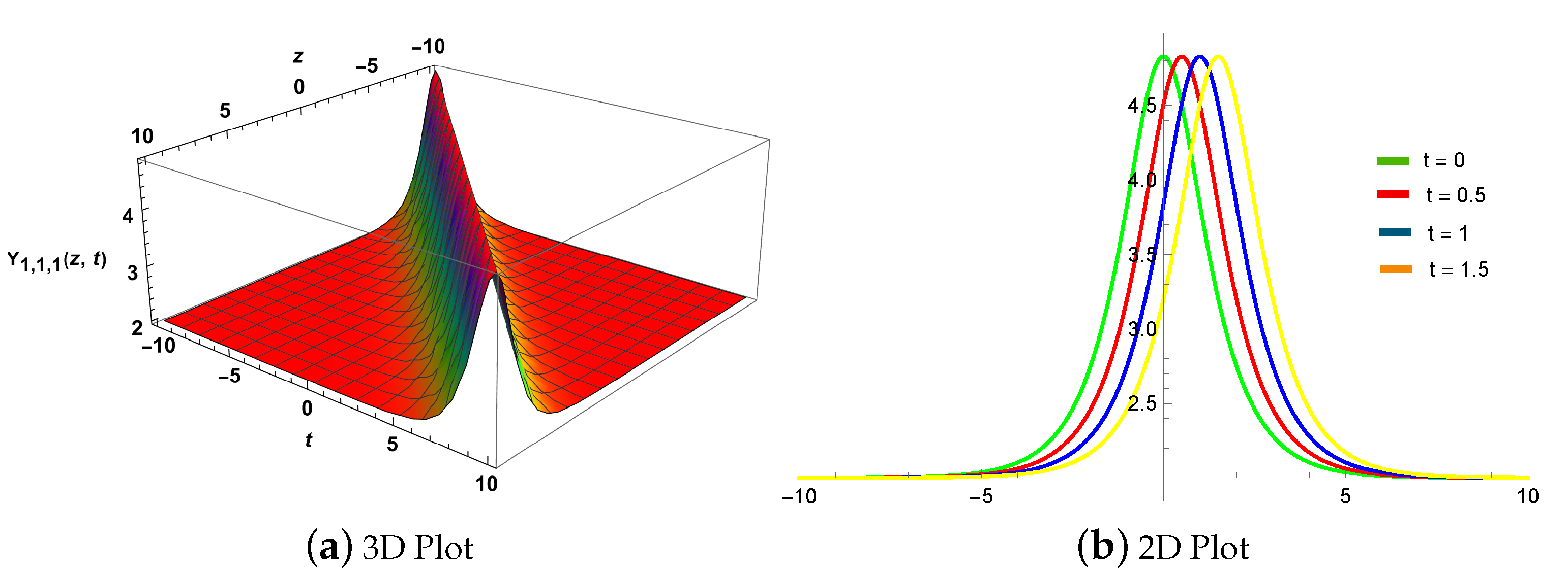
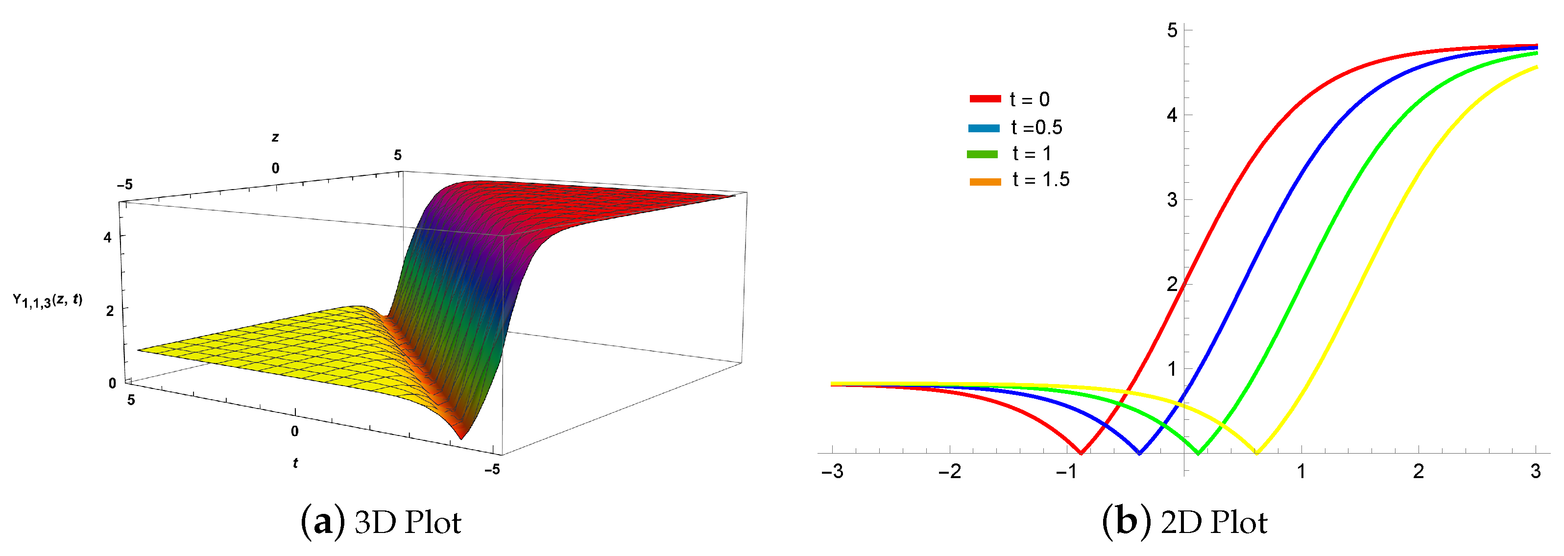
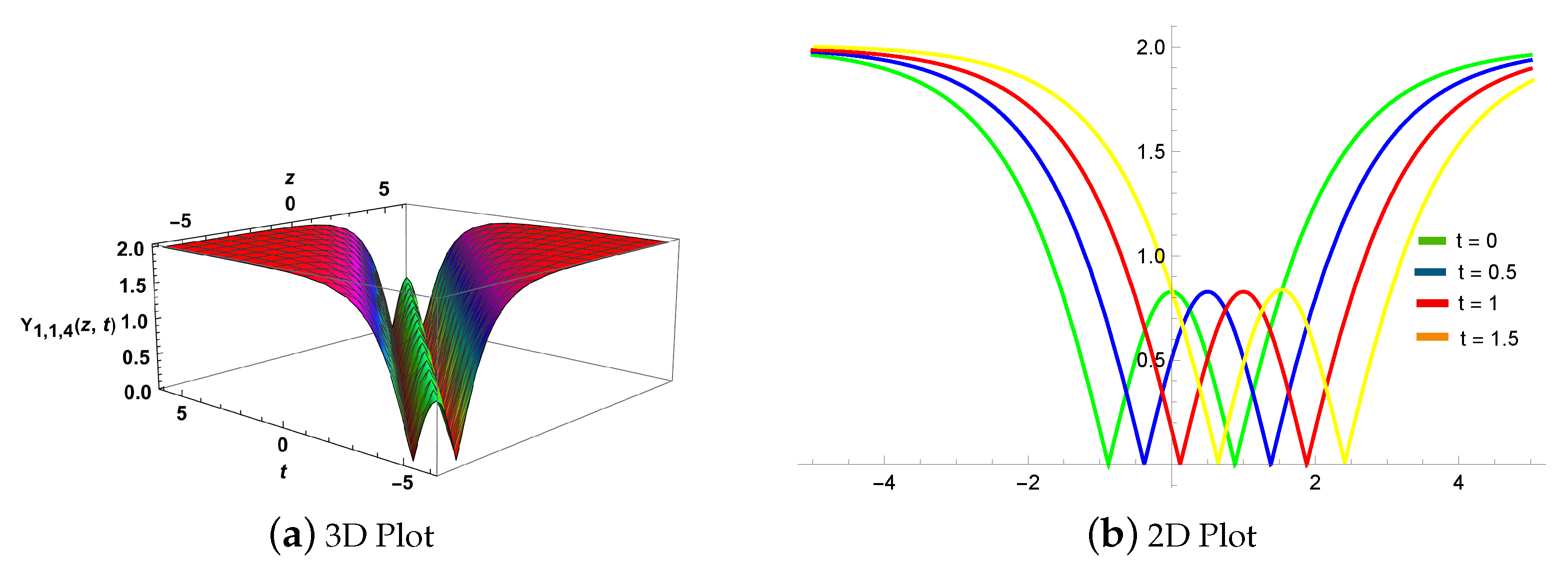
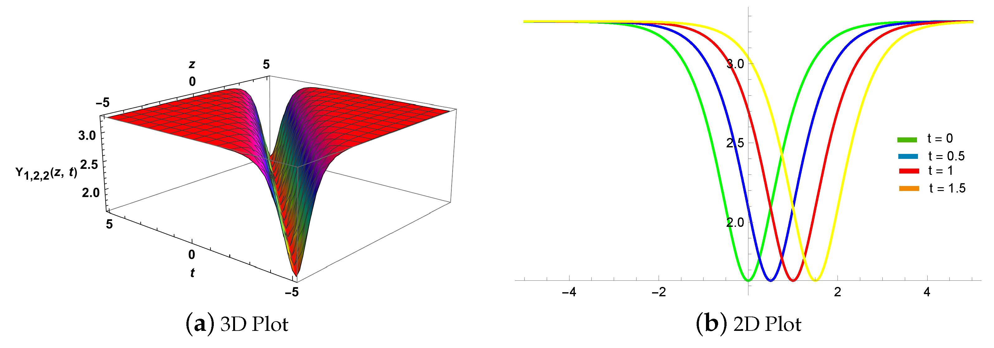
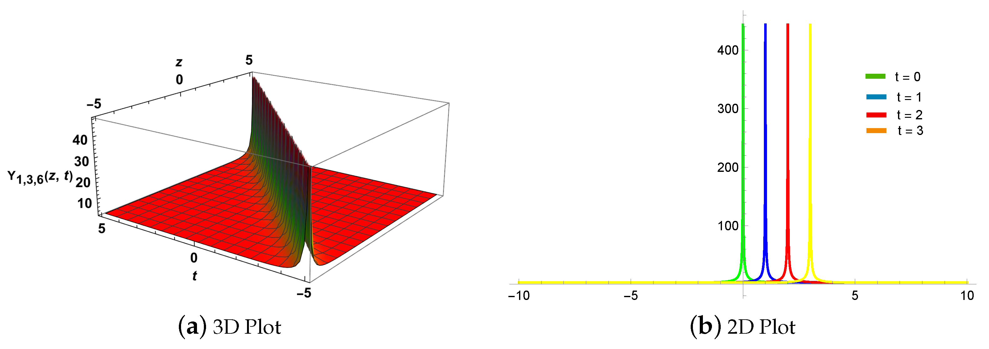
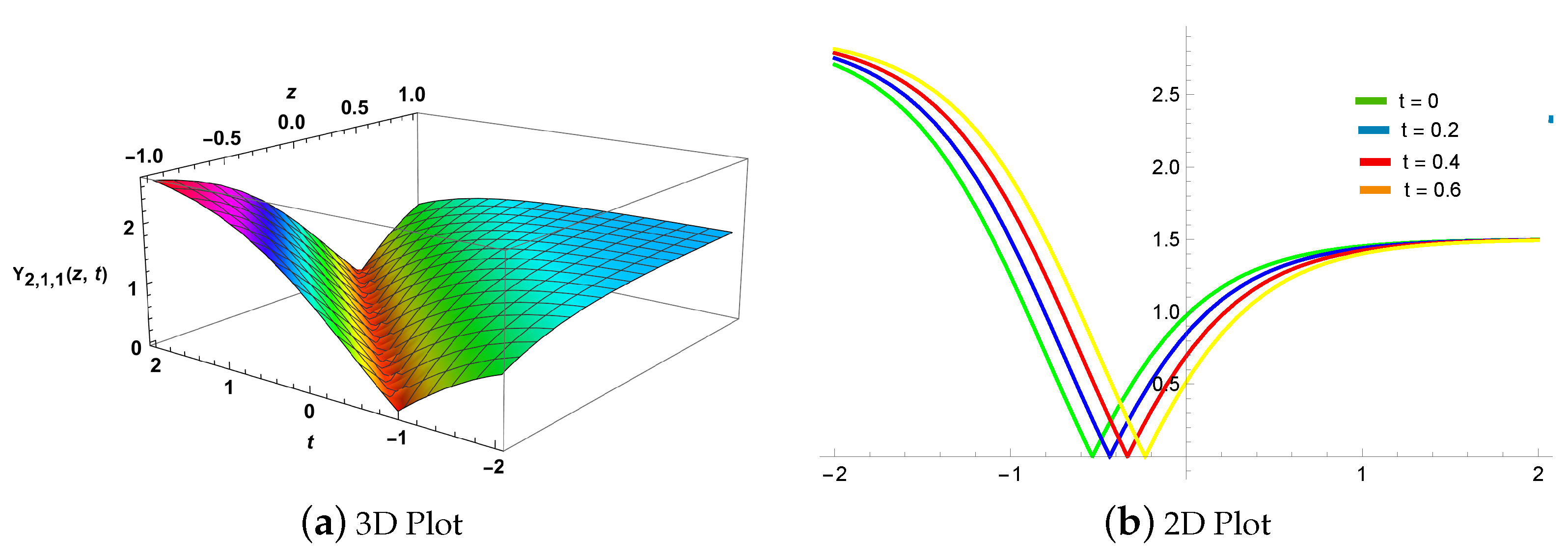
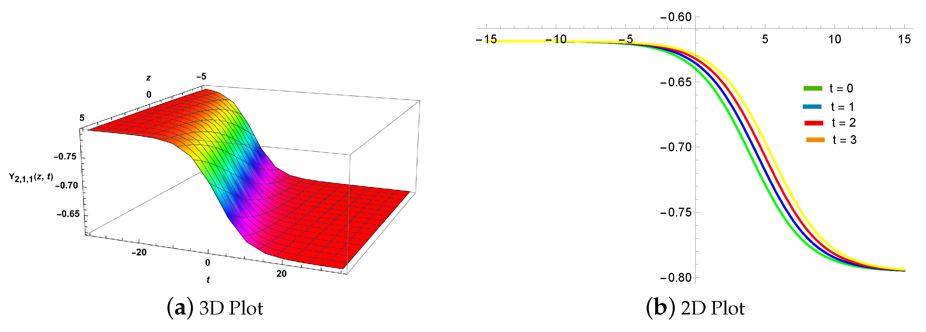
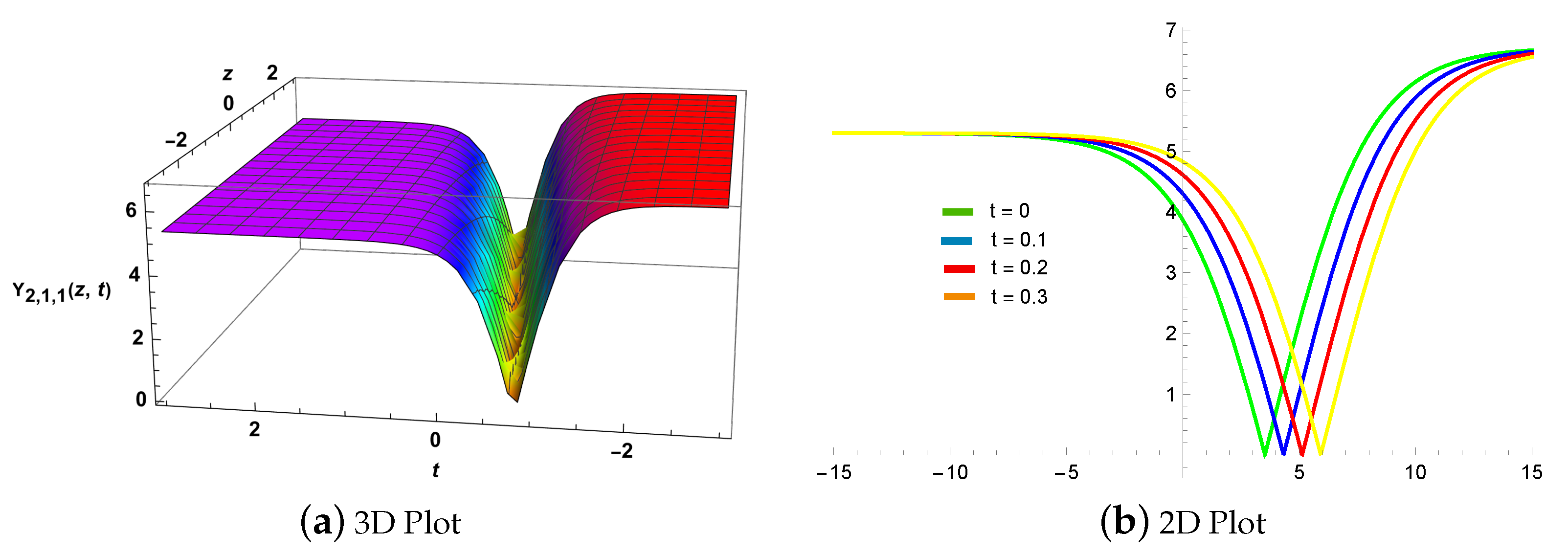
5. Graphical Findings and Discussion

This section examines the graphics illustrations of the GRDM. The graphical behavior associated with the GRDM is generated through the mapping and BS-ODE approaches for different parametric estimates to produce the TW solutions. The Mathematica 13.2 computer software is used to examine their structural architecture in relation to changing the rules governing parameter values. The graphs’ visual appearance will be altered by varying the parameters that are used. For easier understanding, we have shown 3D plots and 2D line graphs. By providing the various values to parameters, a variety of wave profiles can be constructed. By putting the MM and BS-ODE methods into practice, several soliton solutions such as kink type solitons (semi-local nonlinear mode with several decaying oscillation tails and a sharp turn in the waveform between a fixed bottom height), anti-bell shape or dark solitons (localized intensity hole on a continuous wave background), W-shape, bell-shape or bright soliton (localized intensity peak on a homogeneous background), peakon (having discontinuous first derivative) and anti-peakon solitons are obtained.

Figure 1 illustrates the 2D and 3D plots of Equation (23) while using the parametric values $j=1.5,k=2,h=0.5,B=1,K=1$ and $a=1$ within the range $-10\le z\le 10$, $-10\le t\le 10$ using MM, which displays a bell shape or bright soliton. Figure 2 illustrates the 2D and 3D plots of Equation (24) while using the parametric values $j=1.5,k=-2,$$h=0.5,B=1,K=1$ and $a=1$ within the range $-10\le z\le 10$, $-10\le t\le 10$ using MM, which displays a kink type soliton. Figure 3 illustrates the 2D and 3D plots of Equation (25) while using the parametric values $j=1.5,k=2n^2,n=1,h=0.5,B=1,K=1$ and $a=1$ within the range $-2\le z\le 2$, $-2\le t\le 2$ using MM, which displays a peakon type soliton. Figure 4 illustrates the 2D and 3D plots of Equation (26) while using the parametric values $j=1.5,$$k=-2n^2,n=1,h=0.5,B=1,K=1$ and $a=1$ within the range $-5\le z\le 5$, $-5\le t\le 5$ using MM, which displays a W-shape soliton. Figure 5 illustrates the 2D and 3D plots of Equation (28) while using the parametric values $j=-2,k=2,h=0.5,B=1,K=1$ and $a=1$ within the range $-5\le z\le 5$, $-5\le t\le 5$ using MM, which displays a singular shape soliton. Figure 6 illustrates the 2D and 3D plots of Equation (30) while using the parametric values $j=1.5,k=2,h=0.5$, $B=1$, $K=1,a=1$ and $e=1$ within the range $-10\le z\le 10$, $-10\le t\le 10$ using MM, which displays a W-shape soliton. Figure 7 illustrates the 2D and 3D plots of Equation (31) while using the parametric values $j=1.5,k=-2,h=0.5,$$B=1,K=1$ and $e=1$ within the range $-5\le z\le 5$, $-5\le t\le 5$ using MM, which displays an anti-bell or dark soliton. Figure 8 illustrates the 2D and 3D plots of Equation (32) while using the parametric values $j=1.5,k=2n^2,n=1,h=0.5,B=1,K=1,a=1$ and $e=1$ within the range $-2\le z\le 2$, $-5\le t\le 5$ using MM, which displays an anti-peakon type soliton. Figure 9 illustrates the 2D and 3D plots of Equation (38) while using the parametric values $j=1.5,k=-2,h=0.5,B=1,K=1,a=1$ and $e=1$ within the range $-5\le z\le 5$, $-10\le t\le 10$ and $-2\le z\le 2$, $-2\le t\le 2$ using MM, which displays anti-kink and dark solitons. Figure 10 illustrates the 2D and 3D plots of Equation (42) while using the parametric values $j=-2,k=2,h=0.5,B=1,K=1$ and $a=1$ within the range $-5\le z\le 5$, $-5\le t\le 5$ using MM, which displays a singular shape soliton. Figure 11 illustrates the 2D and 3D plots of Equation (47) while using the parametric values $P=0.75,F=0.25,k=0.5,$$\lambda =-5,\mu =5,s=2$ and $q=1$ within the range $-1\le z\le 1$, $-2\le t\le 2$ using BS-ODE, which displays a V-shape soliton. Figure 12 illustrates the 2D and 3D plots of Equation (47) while using the parametric values $P=0.75,F=0.25,k=0.5,\lambda =1,\mu =2,s=2$ and $q=1$ within the range $-5\le z\le 5$, $-20\le t\le 20$ using BS-ODE, which displays an anti-kink type soliton. Figure 13 illustrates the 2D and 3D plots of Equation (47) while using the parametric values $P=4,F=4,k=0.5,\lambda =1,\mu =2,s=-2$ and $q=1$ within the range $-2\le z\le 2$, $-2\le t\le 2$ using BS-ODE, which displays a peakon soliton. Figure 14 illustrates the 2D and 3D plots of Equation (47) while using the parametric values $P=0.75,F=0.25,k=0.5,\lambda =-5,$$\mu =5,s=2$ and $q=1$ within the range $-1\le z\le 1$, $-40\le t\le 40$ using BS-ODE, which displays an anti-peakon soliton. Figure 15 illustrates the 2D and 3D plots of Equation (56) while using the parametric values $P=4,F=4,k=0.5,\lambda =1,\mu =2,s=-2$ and $q=1$ within the range $-5\le z\le 5$, $-5\le t\le 5$ using BS-ODE, which displays an anti-bell or dark soliton.

Additionally, Figure 1, Figure 2, Figure 3, Figure 4, Figure 5, Figure 6, Figure 7, Figure 8, Figure 9, Figure 10, Figure 11, Figure 12, Figure 13, Figure 14 and Figure 15 displays the 2D visualization of solutions for four distinct values of t, representing the impact of time on the soliton’s shape.

6. Analogy of Present and Previous Results

Several researchers examined GRDMs and obtained precise solutions, i.e., Tian and Gao [43] obtained several families of exact solitonic solutions including shock waves, bell-shaped waves and complex valued solutions by using the generalized hyperbolic-function method. Aminikhah, et al. [42] obtained traveling wave solutions to the GRDM by using the functional variable method. Kim and Hong [44] used the auxiliary function method that is another effective method to derive the solutions to the GRDM. Yan and Zhang [45] solved a particular form of the GRDM using a new ansatz and expressed the solutions in explicit forms while, in this study, the exact solutions for the GRDM have been achieved by the mapping and BS-ODE methods. These often-utilized mathematical techniques have been suggested, allowing us to perform complex and time-consuming algebraic calculations. Both approaches have been successfully utilized while working with differential equations. The results indicate that, compared to previous approaches, the mapping and BS-ODE techniques provide better accuracy and need less processing power. There is no need to apply the initial and boundary conditions at the outset. With a wide range of free parameter values, the outcomes that have been obtained include the forms of trigonometric and hyperbolic functions for the BS-ODE technique as well as hyperbolic and Jacobi elliptic functions via the mapping method. As a result, precise types of solitary waves such as dark, bright, kink, anti-kink, V-shaped, peakon, anti-peakon and W-shaped solitons have been established. Figure 1, Figure 2, Figure 3, Figure 4, Figure 5, Figure 6, Figure 7, Figure 8, Figure 9, Figure 10, Figure 11, Figure 12, Figure 13, Figure 14 and Figure 15 have been created to show how the parametric variables, in particular for various values, affect the soliton’s form using Mathematica capabilities. These results have been utilized in mechanical engineering and can contribute to a better understanding of the variety of events that arise in the many physical systems encompassed by the present framework.

7. Stability Analysis

The stability analysis [46] for governing Equation (1) will be examined in this section. Consider the perturbed solution of the form

$${\rm Y}\left(z,t\right)=\vartheta \beta \left(z,t\right)+L_0.$$

(58)

It can be easily seen that any constant $L_0$ is a steady state solution for Equation (1). Plugging Equation (58) into Equation (1) yields

$$\vartheta {\beta }_{tt}+a\vartheta {\beta }_{zz}+a\vartheta \beta +e{L}_0+g{\vartheta }^2{\beta }^2+g{L}_0^2+2g\vartheta \beta L_0+h{\vartheta }^3{\beta }^3+h{L}_0^3+3h{\vartheta }^2{\beta }^2{L}_0+3h\vartheta \beta L_0^2=0.$$

(59)

Linearizing Equation (59) in $\vartheta$,

$$\vartheta {\beta }_{tt}+a\vartheta {\beta }_{zz}+e\vartheta \beta +2g\vartheta \beta L_0+3h\vartheta \beta L_0^2=0.$$

(60)

And let Equation (60) have a solution of the form

$$\beta \left(z,t\right)=e^{i\left(\wp z+\hslash t\right)},$$

(61)

where ℘ is the normalized wave number, plugging Equation (61) into Equation (60),

$$-\vartheta {\hslash }^2-a{\wp }^2+e\vartheta +2g\vartheta L_0+3h\vartheta L_0^2=0.$$

(62)

Solving Equation (62) for ℏ, we obtain

$$\hslash =\sqrt{-\frac{a{\wp }^2}{\vartheta }+e+2g{L}_0+3h{L}_0^2}.$$

(63)

From Equation (63), one can see that, for all $\wp >0$, ℏ is positive. Thus, the dispersion is unstable.

8. Conclusions

In this article, the mapping and Bernoulli sub-ODE approaches are utilized to find unique generalized traveling wave solutions to the generalized reaction Duffing model. These approaches have the major benefit over alternative approaches that these methodologies consistently produce more comprehensive, creative, general solutions and accurate outcomes. On a range of parametric values, several soliton solutions have been developed. Numerous innovative solutions include the kink wave, anti-kink wave, bell shape, anti-bell shape, W-shape, bright, dark and singular shape soliton solutions, produced via the mapping and BS-ODE approaches. Graphic displays of several TW solutions are provided. With the usage of Mathematica 13.2, a basic computational program, the accuracy of these TW solutions results is confirmed. Moreover, there are visual representations in 2D and 3D that show the dynamic behavior of the observed TW solutions. The established wave solutions are more generic than the reachable results in the literature, and distinct values of the associated parameters are originated and a few existing solutions are restored. This study provides evidence of the efficiency, clarity, coherence and consistency of the mapping and BS-ODE techniques. It was evident from the results that several of the TW solutions mentioned are distinct and have not been observed before. It is possible to assess the range of stability and applicability by applying the proposed methodologies to other NLEE kinds, which is a reason for more research. These approaches will be used in the future to find the TW solutions for various problems including quantum mechanics, engineering, neurology and ophthalmology.

References

1. Malik, S.; Hashemi, M.S.; Kumar, S.; Rezazadeh, H.; Mahmoud, W.; Osman, M.S. Application of new Kudryashov method to various nonlinear partial differential equations. Opt. Quantum Electron. 2023, 55, 8. [Google Scholar] [CrossRef]
2. Mollenauer, L.F.; Gordon, J.P. Solitons in Optical Fibers: Fundamentals and Applications; Elsevier Academic Press: Berkeley, CA, USA, 2006. [Google Scholar]
3. Wein, F.; Dunning, P.D.; Norato, J.A. A review on feature-mapping methods for structural optimization. Struct. Multidiscip. Optim. 2020, 62, 1597–1638. [Google Scholar] [CrossRef]
4. He, J.H.; Wu, X.H. Exp-function method for nonlinear wave equations. Chaos Solitons Fractals 2006, 30, 700–708. [Google Scholar] [CrossRef]
5. Bekir, A. New solitons and periodic wave solutions for some nonlinear physical models by using the sine–cosine method. Phys. Scr. 2008, 77, 045008. [Google Scholar] [CrossRef]
6. Guo, M.; Dong, H.; Liu, J.; Yang, H. The time-fractional mZK equation for gravity solitary waves and solutions using sech-tanh and radial basic function method. Nonlinear Anal. Model. Control 2019, 24, 1–19. [Google Scholar] [CrossRef]
7. Zahran, E.H.; Khater, M.M. Modified extended tanh-function method and its applications to the Bogoyavlenskii equation. Appl. Math. Model. 2016, 40, 1769–1775. [Google Scholar] [CrossRef]
8. Abdou, M.A. The extended F-expansion method and its application for a class of nonlinear evolution equations. Chaos Solitons Fractals 2007, 31, 95–104. [Google Scholar] [CrossRef]
9. Zayed, E.M.E.; Arnous, A.H. DNA dynamics studied using the homogeneous balance method. Chin. Phys. Lett. 2012, 29, 080203. [Google Scholar] [CrossRef]
10. Hussain, A.; Chahlaoui, Y.; Zaman, F.D.; Parveen, T.; Hassan, A.M. The Jacobi elliptic function method and its application for the stochastic NNV system. Alex. Eng. J. 2023, 81, 347–359. [Google Scholar] [CrossRef]
11. Biswas, A.; Yildirim, Y.; Yasar, E.; Zhou, Q.; Moshokoa, S.P.; Belic, M. Optical solitons for Lakshmanan–Porsezian–Daniel model by modified simple equation method. Optik 2018, 160, 24–32. [Google Scholar] [CrossRef]
12. Turkyilmazoglu, M. Parametrized adomian decomposition method with optimum convergence. ACM TRansactions Model. Comput. Simul. 2017, 27, 1–22. [Google Scholar] [CrossRef]
13. Iqbal, M.S.; Seadawy, A.R.; Baber, M.Z.; Qasim, M. Application of modified exponential rational function method to Jaulent–Miodek system leading to exact classical solutions. Chaos Solitons Fractals 2022, 164, 112600. [Google Scholar] [CrossRef]
14. Marinca, V.; Herisanu, N.; Marinca, V.; Herisanu, N. Optimal Homotopy Asymptotic Method; Springer International Publishing: New York, NY, USA, 2015; pp. 9–22. [Google Scholar]
15. Aderyani, S.R.; Saadati, R.; Vahidi, J.; Allahviranloo, T. The exact solutions of the conformable time-fractional modified nonlinear Schrödinger equation by the Trial equation method and modified Trial equation method. Adv. Math. Phys. 2022, 2022, 4318192. [Google Scholar] [CrossRef]
16. He, J.H.; Latifizadeh, H. A general numerical algorithm for nonlinear differential equations by the variational iteration method. Int. J. Numer. Methods Heat Fluid Flow 2020, 30, 4797–4810. [Google Scholar] [CrossRef]
17. Akinfe, K.T. A reliable analytic technique for the modified prototypical Kelvin–Voigt viscoelastic fluid model by means of the hyperbolic tangent function. Partial. Differ. Equations Appl. Math. 2023, 7, 100523. [Google Scholar] [CrossRef]
18. Ma, W.X.; Zhang, Y.J. Darboux transformations of integrable couplings and applications. Rev. Math. Phys. 2018, 30, 1850003. [Google Scholar] [CrossRef]
19. Ashraf, R.; Hussain, S.; Ashraf, F.; Akgül, A.; El Din, S.M. The extended Fan’s sub-equation method and its application to nonlinear Schrödinger equation with saturable nonlinearity. Results Phys. 2023, 52, 106755. [Google Scholar] [CrossRef]
20. Wazwaz, A.M. The Hirota’s bilinear method and the tanhcoth method for multiple-soliton solutions of the Sawada–Kotera–Kadomtsev–Petviashvili equation. Appl. Math. Comput. 2008, 200, 160–166. [Google Scholar]
21. Akram, G.; Sadaf, M.; Zainab, I. The dynamical study of Biswas–Arshed equation via modified auxiliary equation method. Optik 2022, 255, 168614. [Google Scholar] [CrossRef]
22. Rani, A.; Zulfiqar, A.; Ahmad, J.; Hassan, Q.M.U. New soliton wave structures of fractional Gilson-Pickering equation using tanh-coth method and their applications. Results Phys. 2021, 29, 104724. [Google Scholar] [CrossRef]
23. Yin, Y.H.; Lü, X.; Ma, W.X. Bäcklund transformation, exact solutions and diverse interaction phenomena to a (3+1)-dimensional nonlinear evolution equation. Nonlinear Dyn. 2022, 108, 4181–4194. [Google Scholar] [CrossRef]
24. Fokas, A.S.; Its, A.R.; Kapaev, A.A.; Novokshenov, V.Y. Painlevé Transcendents: The Riemann-Hilbert Approach; American Mathematical Society: Providence, RI, USA, 2023; Volume 128. [Google Scholar]
25. Alaroud, M. Application of Laplace residual power series method for approximate solutions of fractional IVP’s. Alex. Eng. J. 2022, 61, 1585–1595. [Google Scholar] [CrossRef]
26. Liu, H.; Geng, X. Initial–boundary problems for the vector modified Korteweg–de Vries equation via Fokas unified transform method. J. Math. Anal. Appl. 2016, 440, 578–596. [Google Scholar] [CrossRef]
27. Huang, S.; Chaudhary, K.; Garmire, L.X. More is better: Recent progress in multi-omics data integration methods. Front. Genet. 2017, 8, 84. [Google Scholar] [CrossRef]
28. Kovacic, I.; Brennan, M.J. The Duffing Equation: Nonlinear Oscillators and Their Behaviour; John Wiley & Sons: Hoboken, NJ, USA, 2011. [Google Scholar]
29. Long-Jye, S.; Hsien-Keng, C.; Juhn-Horng, C.; Lap-Mou, T. Chaotic dynamics of the fractionally damped Duffing equation. Chaos Solitons Fractals 2007, 32, 1459–1468. [Google Scholar]
30. Mohammed, W.W.; Al-Askar, F.M.; Cesarano, C. The analytical solutions of the stochastic mKdV equation via the mapping method. Mathematics 2022, 10, 4212. [Google Scholar] [CrossRef]
31. Rehman, H.U.; Saleem, M.S.; Zubair, M.; Jafar, S.; Latif, I. Optical solitons with Biswas–Arshed model using mapping method. Optik 2019, 194, 163091. [Google Scholar] [CrossRef]
32. Zayed, E.M.; Alurrfi, K.A. Solitons and other solutions for two nonlinear Schrödinger equations using the new mapping method. Optik 2017, 144, 132–148. [Google Scholar] [CrossRef]
33. Rabie, W.B.; Khalil, T.A.; Badra, N.; Ahmed, H.M.; Mirzazadeh, M.; Hashemi, M.S. Soliton Solutions and Other Solutions to the (4+1)-Dimensional Davey–Stewartson–Kadomtsev–Petviashvili Equation using Modified Extended Mapping Method. Qual. Theory Dyn. Syst. 2024, 23, 87. [Google Scholar] [CrossRef]
34. Hassan, S.Z.; Abdelrahman, M.A. A Riccati–Bernoulli sub-ODE method for some nonlinear evolution equations. Int. J. Nonlinear Sci. Numer. Simul. 2019, 20, 303–313. [Google Scholar] [CrossRef]
35. Zheng, B. A new Bernoulli sub-ODE method for constructing traveling wave solutions for two nonlinear equations with any order. Univ. Politech. Buchar. Sci. Bull. Ser. A 2011, 73, 85–94. [Google Scholar]
36. Alharbi, A.R.; Almatrafi, M.B. Riccati–Bernoulli sub-ODE approach on the partial differential equations and applications. Int. J. Math. Comput. Sci. 2020, 15, 367–388. [Google Scholar]
37. Peng, Y.Z. Exact solutions for some nonlinear partial differential equations. Phys. Lett. A 2003, 314, 401–408. [Google Scholar] [CrossRef]
38. Khan, K.; Akbar, M.A. Study of explicit travelling wave solutions of nonlinear evolution equations. Partial. Differ. Equations Appl. Math. 2023, 7, 100475. [Google Scholar] [CrossRef]
39. Yousaf, M.Z.; Abbas, M.; Abdullah, F.A.; Nazir, T.; Alzaidi, A.S.; Emadifar, H. Construction of travelling wave solutions of coupled Higgs equation and the Maccari system via two analytical approaches. Opt. Quantum Electron. 2024, 56, 967. [Google Scholar] [CrossRef]
40. Triki, H.; Jovanoski, Z.; Biswas, A. Shock wave solutions to the Bogoyavlensky–Konopelchenko equation. Indian J. Phys. 2014, 88, 71–74. [Google Scholar] [CrossRef]
41. Cakicioglu, H.; Ozisik, M.; Secer, A.; Bayram, M. Kink Soliton Dynamic of the (2+1)-Dimensional Integro-Differential Jaulent-Miodek Equation via a Couple of Integration Techniques. Symmetry 2023, 15, 1090. [Google Scholar] [CrossRef]
42. Aminikhah, H.; Refahi, A.; Rezazadeh, H. Functional variable method for solving the generalized reaction Duffing model and the perturbed Boussinesq equation. Adv. Model. Optim 2015, 17, 55–65. [Google Scholar]
43. Tian, B.; Gao, Y.T. Observable solitonic features of the generalized reaction Duffing Model. Z. Naturforsch. A 2002, 57, 39–44. [Google Scholar] [CrossRef]
44. Kim, J.J.; Hong, W.P. New solitary-wave solutions for the generalized reaction Duffing model and their dynamics. Z. Naturforsch. A 2004, 59, 721–728. [Google Scholar] [CrossRef]
45. Yan, Z.; Zhang, H. Explicit and exact solutions for the generalized reaction duffing equation. Commun. Nonlinear Sci. Numer. Simul. 1999, 4, 224–227. [Google Scholar] [CrossRef]
46. Hussain, E.; Mahmood, I.; Shah, S.A.A.; Khatoon, M.; Az-Zo’bi, E.A.; Ragab, A.E. The study of coherent structures of combined KdV–mKdV equation through integration schemes and stability analysis. Opt. Quantum Electron. 2024, 56, 723. [Google Scholar] [CrossRef]
Figure 1. The imaginary part of solution (23) when j = 1.5 , k = 2 , h = 0.5 , B = 1 and K = 1 produces a bell shape or bright soliton, (a): 3D plot, (b): corresponding 2D line graphs for various values of t.
Symmetry 16 00847 g001
Figure 2. The real part of solution (24) when j = 1.5 , k = 2 , h = 0.5 , B = 1 and K = 1 produces kink wave soliton, (a): 3D plot, (b): corresponding 2D line graphs for various values of t.
Symmetry 16 00847 g002
Figure 3. The absolute of solution (25) when j = 1.5 , k = 2 n 2 , n = 1 , h = 0.5 , B = 1 and K = 1 produces peakon soliton, (a): 3D plot, (b): corresponding 2D line graphs for various values of t.
Symmetry 16 00847 g003
Figure 4. The absolute of solution (26) when j = 1.5 , k = 2 n 2 , n = 1 , h = 0.5 , B = 1 and K = 1 produces a W-shaped soliton, (a): 3D plot, (b): corresponding 2D line graphs for various values of t.
Symmetry 16 00847 g004
Figure 5. The imaginary part of solution (28) when j = 2 , k = 2 , h = 0.5 , B = 1 and K = 1 produces a singular shape soliton, (a): 3D plot, (b): corresponding 2D line graphs for various values of t.
Symmetry 16 00847 g005
Figure 6. The absolute of solution (30) when j = 1.5 , k = 2 , h = 0.5 , B = 1 , K = 1 , a = 1 and e = 1 produces a W-shaped soliton, (a): 3D plot, (b): corresponding 2D line graphs for various values of t.
Symmetry 16 00847 g006
Figure 7. The absolute of solution (31) when j = 1.5 , k = 2 , h = 0.5 , B = 1 , K = 1 and e = 1 produces anti-bell or dark soliton, (a): 3D plot, (b): corresponding 2D line graphs for various values of t.
Symmetry 16 00847 g007
Figure 8. The absolute of solution (32) when j = 1.5 , k = 2 n 2 , n = 1 , h = 0.5 , B = 1 , K = 1 , a = 1 and e = 1 produces anti-peakon soliton, (a): 3D plot, (b): corresponding 2D line graphs for various values of t.
Symmetry 16 00847 g008
Figure 9. The solution of real part and absolute solution of Equation (38) when j = 1.5 , k = 2 , h = 0.5 , B = 1 , K = 1 , a = 1 and e = 1 produces anti-kink and dark solitons, (a,c): 3D plots, (b,d) corresponding: 2D line graphs for various values of t.
Symmetry 16 00847 g009
Figure 10. The absolute solution of Equation (42) when j = 2 , k = 2 , h = 0.5 , B = 1 , K = 1 and a = 1 produces a singular shape soliton, (a): 3D plot, (b): corresponding 2D line graphs for various values of t.
Symmetry 16 00847 g010
Figure 11. The absolute solution of Equation (47) when a = 0.75 , K = 0.25 , B = 0.5 , ρ = 5 , σ = 5 , h = 2 and e = 1 produces a V-shaped soliton, (a): 3D plot, (b): corresponding 2D line graphs for various values of t.
Symmetry 16 00847 g011
Figure 12. The imaginary part of solution (47) when a = 0.75 , K = 0.25 , B = 0.5 , ρ = 1 , σ = 2 , h = 2 and e = 1 produces anti-kink type soliton, (a): 3D plot, (b): corresponding 2D line graphs for various values of t.
Symmetry 16 00847 g012
Figure 13. The absolute solution of Equation (47) when a = 4 , K = 4 , B = 0.5 , ρ = 1 , σ = 2 , h = 2 and e = 1 produces a peakon soliton, (a): 3D plot, (b): corresponding 2D line graphs for various values of t.
Symmetry 16 00847 g013
Figure 14. The absolute solution (47) when a = 0.75 , K = 0.25 , B = 0.5 , ρ = 5 , σ = 5 , h = 2 and e = 1 produces anti-peakon soliton, (a): 3D plot, (b): corresponding 2D line graphs for various values of t.
Symmetry 16 00847 g014
Figure 15. The absolute solution of Equation (56) when a = 4 , K = 4 , B = 0.5 , ρ = 1 , σ = 2 , h = 2 and e = 1 produces anti-bell or dark soliton, (a): 3D plot, (b): corresponding 2D line graphs for various values of t.
Symmetry 16 00847 g015
Disclaimer/Publisher’s Note: The statements, opinions and data contained in all publications are solely those of the individual author(s) and contributor(s) and not of MDPI and/or the editor(s). MDPI and/or the editor(s) disclaim responsibility for any injury to people or property resulting from any ideas, methods, instructions or products referred to in the content.