Soliton Dynamics and Modulation Instability in the (3+1)-Dimensional Generalized Fractional Kadomtsev–Petviashvili Equation

Abstract

In this article, novel methods of analysis to solve the (3+1)-dimensional generalized fractional Kadomtsev–Petviashvili equation, which plays a crucial role in the modelling of fluid dynamics, particularly wave propagation in complicated media, are presented. The fractional KP equation, a well-established mathematical model, uses fractional derivatives to more adequately describe more general types of nonlinear wave phenomena, with a richer and improved understanding of the dynamics of fluids with non-classical characteristics, such as anomalous diffusion or long-range interactions. Two efficient methods, the exponential rational function technique (ERFT) and the generalized Kudryashov technique (GKT), have been applied to find exact travelling solutions describing soliton behaviour. Solitons, localized waveforms that do not deform during propagation, are central to the dynamics of waves in fluid systems. The characteristics of the obtained results are explored in depth and presented both by three-dimensional plots and by two-dimensional contour plots. Plots provide an explicit picture of how the solitons evolve in space and time and provide insight into the underlying physical phenomena. We also added modulation instability. Our analysis of modulation instability further underscores the robustness and physical relevance of the obtained solutions, bridging theoretical advancements with observable phenomena.

1. Introduction

Recent years have witnessed growing undivided attention being paid to exploring the quest for solitary wave solutions within the domain of nonlinear fractional differential equations (NFDEs) [1,2]. Researchers have devoted significant attention to understanding the formation, propagation, and interaction of solitary waves, which are crucial for modeling a wide range of physical phenomena [3,4]. These include fluid dynamics, plasma physics, and nonlinear optics, where solitary waves often emerge as stable, localized structures that maintain their shape during propagation [5]. The exploration of analytical solutions to these equations has led to the development of various methods, highlighting the importance of solitary wave solutions in understanding complex nonlinear systems [6,7]. Over the years, numerous successful strategies have been developed to investigate and obtain exact solutions of NFDEs. These methods range from classical analytical approaches, such as the sine-Gordon equation technique [8], Hirota simplified method [9], first integral technique [10], sub-equation technique [11], modified auxiliary equation procedure [12,13], new extended algebraic technique [14], modified expansion function method [15], modified Kudryashov technique [16], ${\varphi }^6$—model expansion method [17], modified trial equation technique [18], modified simple equation method [19], Hirota method [20,21], unified Riccati equation expansion method [22], extended Riccati equation method [23], ($m+{\displaystyle \frac{G^{\prime }}{G}}$)-expansion method [24], and so on.

The primary objective of this study is to examine wave propagation in the context of the (3+1)-dimensional generalized fractional KP equation. For this purpose, we employed analytical solutions, plotted the obtained results, and provided the modulation instability. The manuscript is organized as follows: Section 2 delves into the theory and characteristics of beta derivatives. Section 3 offers preliminary details. In Section 4, there is a concise exploration of ERFT and GKT, along with a graphical analysis of the proposed model. Then, modulation instability is given. Lastly, the discussion and conclusion encapsulates the summarized findings.

The work significantly advances the study of nonlinear fractional systems considering the reduction of such equations to ordinary differential equations and the obtaining of exact solutions by symbolic computation. The capability of our analytical techniques is mirroring the obtaining of new travelling wave solutions that are very relevant in mathematical physics on account of their unique physical properties of self-amplification, shape-preservation, and constant-velocity propagation owing to balanced dispersion and nonlinear effects. Beyond mathematical beauty, these solutions explain wave dynamics in fractional-order media and the insight provided by them can be useful for practical works in optical communication, plasma physics, and fluid dynamics. On the other hand, the study of modulation instability gives much more confidence and physical relevance to the derived solutions linking theory to observable behaviour. By joining computation and analysis rigorously, this study does not only upscale the toolbox for fractional nonlinear systems, but it also creates a path toward the study of complex interactions of waves within disordered or nonlocal environments in the future.

2. Preliminaries

In this research paper, (3+1)-dimensional generalized fractional Kadomtsev–Petviashvili equations are examined [25]:

$${\left[{\displaystyle \frac{{\partial }^{\alpha }u}{\partial t^{\alpha }}}+ϵu{u}_x+\delta u_{xxx}\right]}_x+\nu u_{yy}+{\tau }_1{u}_{xx}+{\tau }_2{u}_{xy}+{\tau }_3{u}_{xz}=0.$$

(1)

In recent years, some researchers studied Equation (1) using various methods. For example, Xu and Wazwaz recently studied the Painleve integrability of Equation (1) and obtained its N-soliton solutions [26]. Hong and Wang applied the Jacobi elliptic function expansion method to the (3+1)-dimensional fractional Kadomtsev–Petviashvili (KP) equation, which provided a plethora of solitary wave solutions. They generalized the use of this method to fractional PDEs, giving new insight into the propagation of nonlinear waves. By using this method, they could find new forms of solitary wave solutions that can be utilized to describe complex wave phenomena in different physical systems [27].

The (3+1)-dimensional fractional Kadomtsev–Petviashvili (KP) equation has attracted much attention in recent years, playing an important role in describing various nonlinear phenomena in different scientific fields. A very interesting equation, with wide applications in fields such as mechanical fluid dynamics and plasma, is the KP-type equation [27]. The equation has a basic role in describing the propagation of long waves with small amplitudes in various plasma systems when perturbations are considered in two-dimensional space [28]. Because of the wide applications of the KP-type equation, researchers have explored research works relying on extensions and generalizations of the KP structure [29]. These excursions have yielded valuable insights, allowing the exploration of novel physical properties observed in diverse applications. Given the extensive utility of the KP-type equation, researchers have delved into studies exploring extensions and generalizations of the KP structure [29]. These explorations have yielded valuable insights, facilitating the examination of novel physical characteristics observed in numerous applications.

The fractional derivatives introduce additional complexity that can capture nonlocal effects or memory-dependent behaviour in the wave propagation process. These fractional derivatives can model situations where the response of the system is not instantaneous, but instead depends on past states, often seen in systems with anomalous diffusion or long-range interactions [29]. Hao et al. studied the Painleve analysis of the equation [30].

2.1. Some Useful Properties of the Beta Derivative

The beta-derivative (or conformable fractional derivative with beta kernel) was adopted in our work due to its computational simplicity and preservation of classical derivative properties (e.g., chain rule, Leibniz rule) while still capturing nonlocal effects. Unlike classical fractional derivatives (e.g., Riemann–Liouville, Caputo), the beta-derivative avoids singular kernels and is defined for functions without requiring fractional initial conditions [3,4,5].

Definition 1.

When $\varsigma \left(t\right)$ is a function dependent on t which is different from the negative constant, the β derivative of $\varsigma \left(t\right)$ is defined as follows:

$$T^{\beta }\left(\varsigma \left(t\right)\right)=\underset{\epsilon \to 0}{lim}{\displaystyle \frac{\varsigma \left(t+\epsilon {\left(t+\frac{1}{\Gamma \left(\beta \right)}\right)}^{1-\beta }\right)-\varsigma \left(t\right)}{\epsilon }},0<\beta \le 1,$$

(2)

where the β derivative is represented by $T^{\beta }\left(\varsigma \left(t\right)\right)={\displaystyle \frac{d^{\beta }\varsigma \left(t\right)}{d{t}^{\beta }}}$.

Certain features are outlined below:

Theorem 1

([4,31]). Let $\varsigma \left(t\right)$ and $\upsilon \left(t\right)$ be β-differentiable functions for all $t>0$ and $\beta \in (0,1]$:

$1.$ $T^{\beta }(a\varsigma \left(t\right)+b\upsilon \left(t\right))=a{T}^{\beta }\left(\varsigma \left(t\right)\right)+b{T}^{\beta }\left(\upsilon \left(t\right)\right),\forall a,b\in R$

$2.$ $T^{\beta }\left(\varsigma \left(t\right)\upsilon \left(t\right)\right)=\upsilon \left(t\right)T^{\beta }\left(\varsigma \left(t\right)\right)+\varsigma \left(t\right)T^{\beta }\left(\upsilon \left(t\right)\right),$

$3.$ $T^{\beta }\left({\displaystyle \frac{\varsigma \left(t\right)}{\upsilon \left(t\right)}}\right)={\displaystyle \frac{\upsilon \left(t\right)T^{\beta }\left(\varsigma \left(t\right)\right)-\varsigma \left(t\right)T^{\beta }\left(\upsilon \left(t\right)\right)}{\upsilon {\left(t\right)}^2}},$

$4.$ $T^{\beta }\left(\varsigma \left(t\right)\right)={\left(t+{\displaystyle \frac{1}{\Gamma \left(\beta \right)}}\right)}^{1-\beta }{\displaystyle \frac{d\varsigma \left(t\right)}{dt}}$.

2.2. Background Information

The time-fractional NFDE with the beta derivative is expressed in its general form as follows [32,33]:

$$F(u,D_t^{\beta }u,D_{x}u,D_t^{\beta }{D}_t^{\beta }u,D_t^{\beta }{D}_{x}u,D_x{D}_{x}u,...)=0,0<\beta \le 1.$$

(3)

Here, F is a polynomial involving partial beta derivatives of $u(x,y,z,t)$. Utilization of the following wave transformation

$$u(x,y,z,t)=u\left(\xi \right),\xi =x+y+z-{\displaystyle \frac{c}{\beta }}{\left(t+{\displaystyle \frac{1}{\Gamma \left(\beta \right)}}\right)}^{\beta },$$

(4)

for Equation (3) provides a nonlinear ordinary differential equation (ODE) as follows:

$$Q\left({\left(u^{\prime }\right)}^2,u^{″},u{u}^{″},u^{\left(4\right)},\dots \right)=0.$$

(5)

3. Proposed Methods

In this section, two distinct techniques for obtaining analytical solutions to NFDEs have been presented. Specifically, the key steps involved in the ERFT and the GKT have been outlined. The ERFT is utilized for its ability to provide solutions in terms of rational functions that involve exponential terms, which is effective for capturing the complex wave interactions in fractional equations. The GKT, on the other hand, is a more refined approach that allows for a broader class of solutions and has been successfully applied to nonlinear equations in various scientific fields. Also, the methods employed in this research take advantage of the equation’s symmetrical structure to derive exact analytical solutions, demonstrating the deep connection between symmetry and nonlinear wave phenomena.

3.1. Generalized Kudryashov Technique

The main steps for the proposed method can be given as follows:

Step 1: Assume that the solution of Equation (5) can be expressed in the subsequent rational form:

$$u\left(\xi \right)={\displaystyle \frac{{\displaystyle \sum _{i=0}^N}{\varrho }_i{R}^i\left(\xi \right)}{{\displaystyle \sum _{j=0}^M}{\rho }_j{R}^j\left(\xi \right)}},$$

(6)

where ${\varrho }_i(i=0,1,...,N),{\rho }_j(j=0,1,...,M)$ are constants to be determined, such that ${\varrho }_N\ne 0$, ${\rho }_M\ne 0$ and $R=R\left(\xi \right)$ satisfies the ODE.

$${\displaystyle \frac{dR}{d\xi }}=R^2\left(\xi \right)-R\left(\xi \right).$$

(7)

The solution of Equation (7) makes it evidently clear that

$$R\left(\xi \right)={\displaystyle \frac{1}{1+A{e}^{\xi }}},$$

(8)

where A is the integration constant.

Step 2: To obtain the positive integers N and M in Equation (6) through the application of the homogeneous balance method, consider the relationship between the highest-order derivatives and the most dominant nonlinear terms in Equation (5).

Step 3: By substituting Equation (6) into Equation (5) along with Equation (7), a polynomial of $R\left(Q\right)$ of Q is acquired. Next, by setting all coefficients of $R\left(Q\right)$ to zero, a system of algebraic equations has been acquired. Finding the solutions of this system with the aid of Maple, the values of ${\varrho }_i(i=0,1,\dots ,N),{\rho }_j(j=0,1,\dots ,M)$ can be found. Finally, by substituting these values and Equation (7) into Equation (6), the exact solutions of the simplified Equation (5) can be found [32].

3.2. Exponential Rational Function Technique

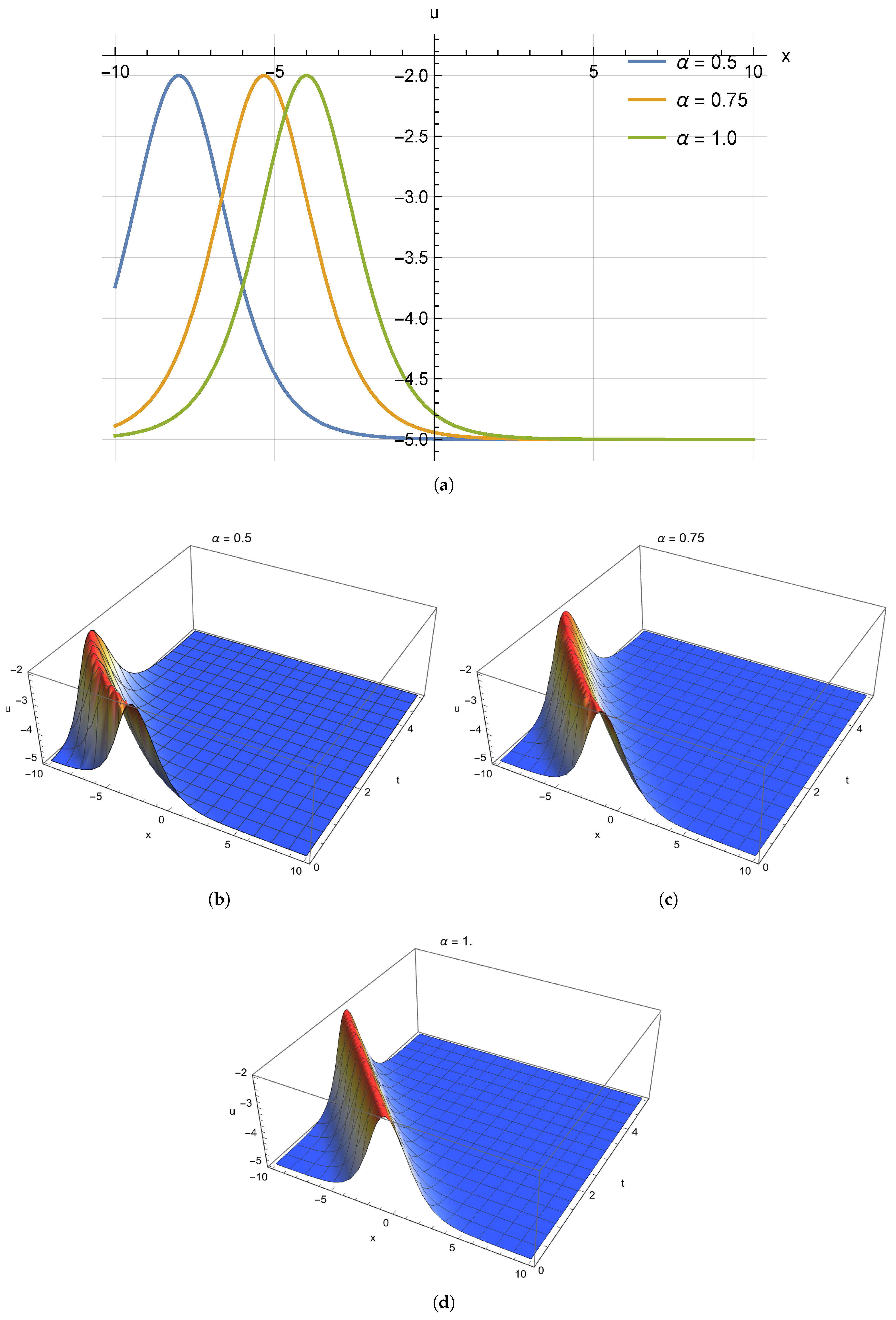
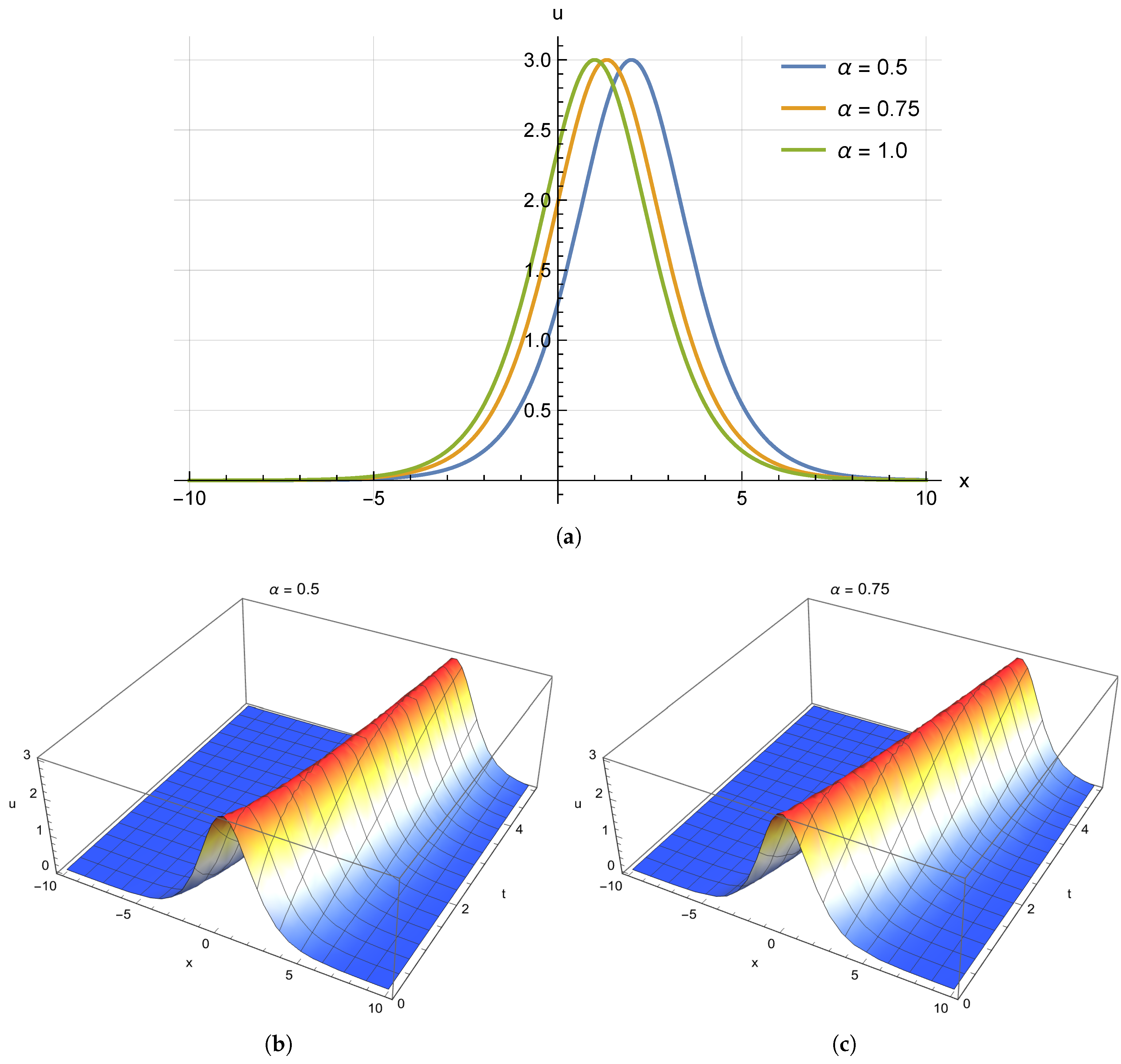
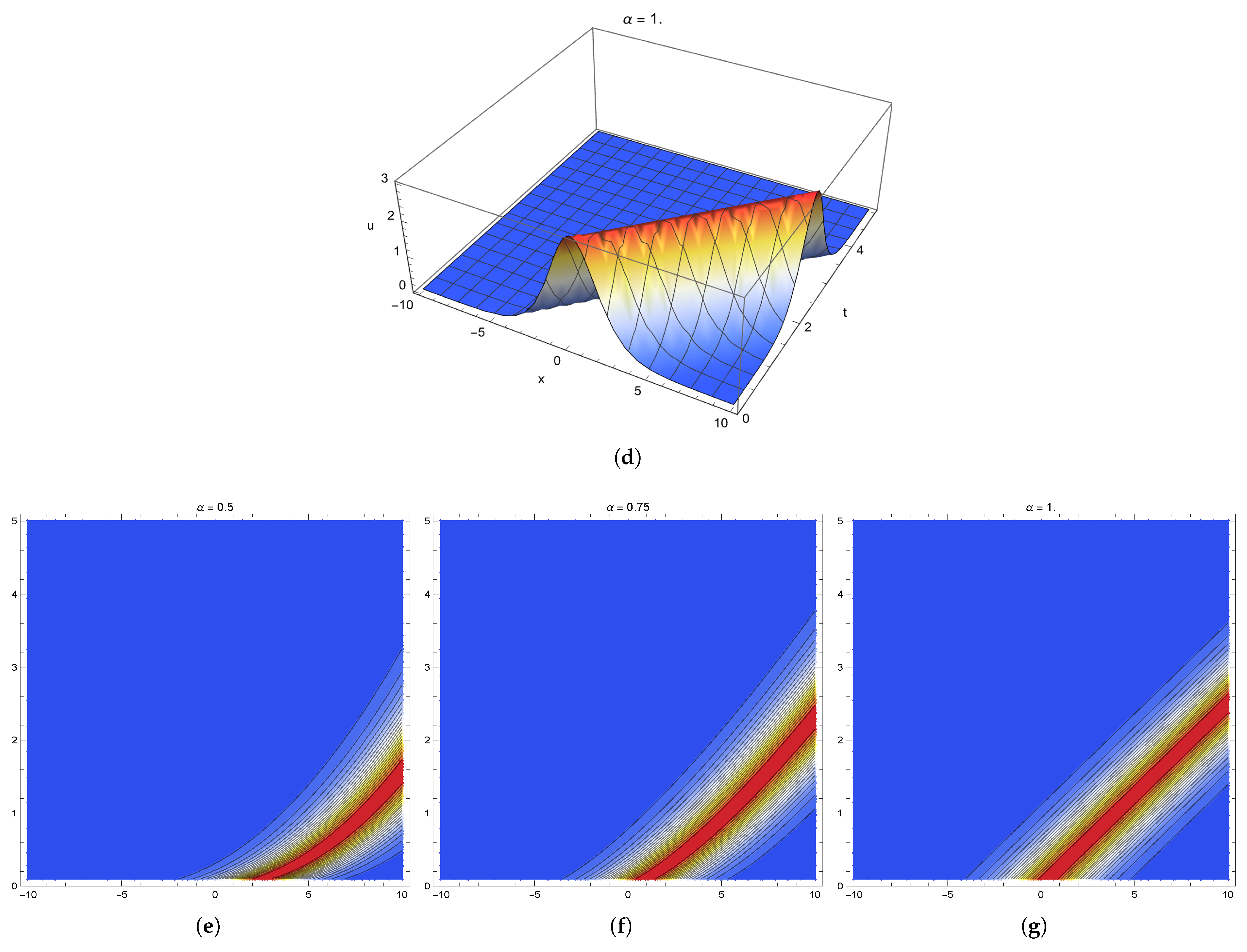
The main steps for the proposed method can be given as follows:

Step 1. The analytical solution to Equation (5) can be represented in the following manner:

$$u\left(\xi \right)=\sum _{n=0}^N{\displaystyle \frac{{\varrho }_n}{{(1+e^{\xi })}^n}},$$

(9)

where ${\varrho }_n$$\left({\varrho }_N\ne 0\right)$ are constants to be determined later. Find the integer N using the homogenous balance principle. This method is given by balancing the highest-order linear term with the highest-order nonlinear term in Equation (5).

Step 2. By substituting Equation (9) into Equation (5) and separating all terms with the same order of $e^{n\xi }$$(n=0,1,2,\dots )$ together, the left-hand side of Equation (5) has been transformed into another polynomial in $e^{n\xi }$. Then, setting each coefficient of this polynomial to zero results in a set of algebraic equations for ${\varrho }_n$ unknown parameters. Ultimately, solving this system enables the construction of a diverse set of exact solutions for Equation (3) [34].

4. Main Results

For this purpose, the transformation defined in Equation (3) was applied to Equation (1). Then, the following ordinary differential equation was verified:

$$u^{″}(-c+v+{\tau }_1+{\tau }_2+{\tau }_3)+ϵ{\left(u^{\prime }\right)}^2+ϵu{u}^{″}+\delta u^{\left(4\right)}=0.$$

(10)

Upon integrating this equation with respect to $\xi$ once, the result was as follows:

$$(-c+\nu +{\tau }_1+{\tau }_2+{\tau }_3+ϵu)u^{\prime }+\delta u^{\left(3\right)}=0.$$

(11)

4.1. Algorithm of Generalized Kudryashov Technique

In accordance with the homogeneous balance principle, the balancing number was found to be $N=M+2$. When M was assigned the value of 1, N became 3. As a result, the solution can be articulated as follows:

$$u\left(\xi \right)={\displaystyle \frac{{\varrho }_0+{\varrho }_{1}R+{\varrho }_2{R}^2+{\varrho }_3{R}^3}{{\rho }_0+{\rho }_{1}R}},$$

(12)

where $R=R\left(\xi \right)$ is the solution of the Equation (7). Utilizing this information, Equation (12) can be substituted into Equation (11) and Equation (7) can be used. Subsequently, by setting all coefficients of the functions $R^k$ to zero, we obtain a system of equations involving the parameters ${\varrho }_0$, ${\varrho }_1$, ${\varrho }_2$, ${\varrho }_3$, ${\rho }_0$ and ${\rho }_1$. Upon resolving this system, the ensuing results are produced:

Case 1:

$$\begin{array}{c}{\varrho }_0={\displaystyle \frac{{\rho }_0\left(-12\delta {\rho }_0+ϵ{\varrho }_1\right)}{ϵ{\rho }_1}},{\varrho }_2=-{\displaystyle \frac{12\delta ({\rho }_1-{\rho }_0)}{ϵ}},{\varrho }_3=-{\displaystyle \frac{12\delta {\rho }_1}{ϵ}},\hfill \\ c={\displaystyle \frac{-12\delta {\rho }_0+\nu {\rho }_1+\delta {\rho }_1+ϵ{\varrho }_1+{\tau }_1{\rho }_1+{\tau }_3{\rho }_1+{\tau }_2{\rho }_1}{{\rho }_1}}.\hfill \end{array}$$

(13)

Hence, the travelling wave solution for the (3+1)-dimensional generalized fractional Kadomtsev–Petviashvili equation can be expressed as follows:

$$u_1(x,y,z,t)={\displaystyle \frac{\frac{{\rho }_0\left(-12\delta {\rho }_0+ϵ{\varrho }_1\right)}{ϵ{\rho }_1}+\frac{{\varrho }_1}{B_1(x,y,z,t)}-\frac{12\delta ({\rho }_1-{\rho }_0)}{ϵB_1^2(x,y,z,t)}-\frac{12\delta {\rho }_1}{ϵB_1^3(x,y,z,t)}}{{\rho }_0+\frac{{\rho }_1}{B_1(x,y,z,t)}}},$$

(14)

where

$$B_1(x,y,z,t)=1+A\left(cosh\left(x+y+z-{\displaystyle \frac{c}{\beta }}{\left(t+{\displaystyle \frac{1}{\Gamma \left(\beta \right)}}\right)}^{\beta }\right)+sinh\left(x+y+z-{\displaystyle \frac{c}{\beta }}{\left(t+{\displaystyle \frac{1}{\Gamma \left(\beta \right)}}\right)}^{\beta }\right)\right)$$

(15)

and A is the integration constant (Figure 1).

Case 2:

$$\begin{array}{c}{\varrho }_0=0,{\varrho }_1={\displaystyle \frac{{\rho }_1(-{\tau }_1-{\tau }_2-{\tau }_3+c-\delta -\nu )}{ϵ}},\hfill \\ {\varrho }_2={\displaystyle \frac{12\delta {\rho }_1}{ϵ}},{\varrho }_3=-{\displaystyle \frac{12\delta {\rho }_1}{ϵ}},{\rho }_0=0.\hfill \end{array}$$

(16)

Hence, the travelling wave solution for the (3+1)-dimensional generalized fractional Kadomtsev–Petviashvili equation can be expressed as follows:

$$u_2(x,y,z,t)=\left({\displaystyle \frac{\frac{{\rho }_1(-{\tau }_1-{\tau }_2-{\tau }_3+c-\delta -\nu )}{ϵB_2(x,y,z,t)}+\frac{12\delta {\rho }_1}{ϵB_2^2(x,y,z,t)}-\frac{12\delta {\rho }_1}{ϵB_2^3(x,y,z,t)}}{{\rho }_1}}\right)B_1(x,y,z,t),$$

(17)

where A is the integration constant (Figure 2).

4.2. Algorithm of Exponential Rational Function Technique

By applying the homogeneous balance principle to Equation (11), the balancing number can be found to be $N=2$. Consequently, the desired solution can be formulated as follows:

$$u\left(\xi \right)={\varrho }_0+{\displaystyle \frac{{\varrho }_1}{1+e^{\xi }}}+{\displaystyle \frac{{\varrho }_2}{{(1+e^{\xi })}^2}}.$$

(18)

Upon substituting Equation (18) into Equation (11), the resulting set of equations can be represented as follows:

$$\begin{array}{ccc}{e}^{4\xi }\hfill & :\hfill & -ϵ{\varrho }_0{\varrho }_1-{\tau }_3{\varrho }_1-{\tau }_2{\varrho }_1-\delta {\varrho }_1-\nu {\varrho }_1+c{\varrho }_1-{\tau }_1{\varrho }_1=0,\hfill \\ \hfill & \hfill & \\ e^{3\xi }\hfill & :\hfill & -8\delta {\varrho }_2-3{\tau }_1{\varrho }_1-3{\tau }_2{\varrho }_1-3ϵ{\varrho }_0{\varrho }_1+3\delta {\varrho }_1-3{\tau }_3{\varrho }_1+3c{\varrho }_1-2{\tau }_2{\varrho }_2\hfill \\ \hfill & \hfill & -2ϵ{\varrho }_0{\varrho }_2-3\nu {\varrho }_1+2c{\varrho }_2-2{\tau }_3{\varrho }_2-2{\tau }_1{\varrho }_2-ϵ{\varrho }_1^2-2\nu {\varrho }_2=0,\hfill \\ \hfill & \hfill & \\ e^{2\xi }\hfill & :\hfill & 4c{\varrho }_2+3c{\varrho }_1-4{\tau }_1{\varrho }_2-3\nu {\varrho }_1-3{\tau }_1{\varrho }_1-4{\tau }_3{\varrho }_2-2ϵ{\varrho }_1^2-4\nu {\varrho }_2+3\delta {\varrho }_1\hfill \\ \hfill & \hfill & -3ϵ{\varrho }_0{\varrho }_1-3ϵ{\varrho }_1{\varrho }_2+14\delta {\varrho }_2-4{\tau }_2{\varrho }_2-3{\tau }_3{\varrho }_1-3{\tau }_2{\varrho }_1-4ϵ{\varrho }_0{\varrho }_2=0,\hfill \\ \hfill & \hfill & \\ e^{\xi }\hfill & :\hfill & c{\varrho }_1+2c{\varrho }_2-\nu {\varrho }_2-2\nu {\varrho }_2-{\tau }_1{\varrho }_2-2{\tau }_1{\varrho }_2-{\tau }_2{\varrho }_2-2{\tau }_2{\varrho }_2-{\tau }_3{\varrho }_2\hfill \\ \hfill & \hfill & -2{\tau }_3{\varrho }_2-ϵ{\varrho }_1^2-2ϵ{\varrho }_2^2-2ϵ{\varrho }_0{\varrho }_2-3ϵ{\varrho }_2{\varrho }_2-\delta {\varrho }_2-ϵ{\varrho }_0{\varrho }_2-2\delta {\varrho }_2=0.\hfill \end{array}$$

Upon resolving this system, the ensuing results are produced:

$${\varrho }_1={\displaystyle \frac{12\delta }{ϵ}},{\varrho }_2=-{\displaystyle \frac{12\delta }{ϵ}},c=ϵ{\varrho }_0+{\tau }_3+{\tau }_2+\delta +v+{\tau }_1.$$

(19)

Hence, the travelling wave solution for the (3+1)-dimensional generalized fractional Kadomtsev–Petviashvili equation can be expressed as follows:

$$u_3(x,y,z,t)={\varrho }_0+{\displaystyle \frac{12\delta }{ϵB_1(x,y,z,t)}}-{\displaystyle \frac{12\delta }{ϵB_1^2(x,y,z,t)}},$$

(20)

where A is the integration constant (Figure 3).

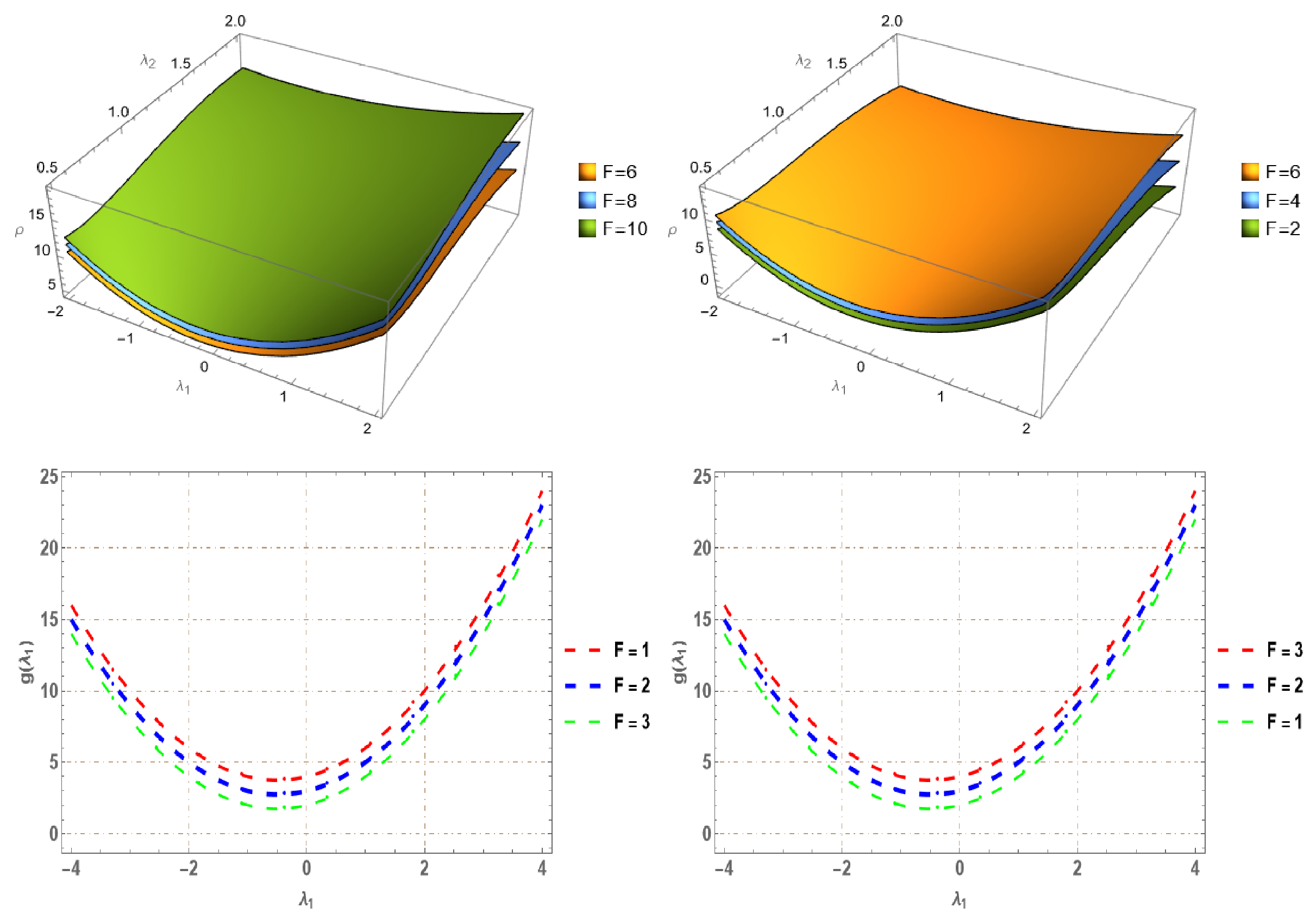
4.3. Modulation Instability

The interplay between dispersive and nonlinear components affects the stability of solutions in nonlinear systems. The phenomenon, known as modulation instability, occurs when a continuous plane wave propagates in a nonlinear dispersive medium and experiences self-modulation in both frequency and amplitude. As a result, the plane wave’s number of tiny disturbances increases exponentially. Examining the modulation instability areas lays the groundwork for handling different nonlinear models or events in various fields. We will focus on the modulation instability of the (3+1)-dimensional generalized fractional Kadomtsev–Petviashvili equation in the (3+1) dimensions.

To evaluate modulation instability, we will look for perturbed solutions that look like this [35]:

$$\begin{array}{c}\hfill \begin{array}{c}\hfill u(x,y,z,t)=F+\vartheta P(x,y,z,t).\end{array}\end{array}$$

(21)

where P represents the perturbation term, $\vartheta <1$ is the perturbation coefficient parameter, and F represents the incident power.

Inserting Equation (21) into the governing model, we obtain

$$\begin{array}{c}\hfill \begin{array}{cc}& \nu \vartheta P_{yy}+ϵ{\vartheta }^2{P}_x^2+\vartheta P_{xt}+\vartheta {\tau }_3{P}_{xz}+\vartheta {\tau }_2{P}_{xy}+Fϵ\vartheta P_{xx}+\vartheta {\tau }_1{P}_{xx}+ϵ{\vartheta }^2{P}_{xx}+\delta \vartheta P_{xxxx}=0.\hfill \end{array}\end{array}$$

(22)

Equation (22) should now be linearized in P.

$$\begin{array}{c}\hfill \begin{array}{cc}& \nu \vartheta P_{yy}+\vartheta P_{xt}+\vartheta {\tau }_3{P}_{xz}+\vartheta {\tau }_2{P}_{xy}+Fϵ\vartheta P_{xx}+\vartheta {\tau }_1{P}_{xx}+\delta \vartheta P_{xxxx}=0.\hfill \end{array}\end{array}$$

(23)

Examine the following as the solution to Equation (23):

$$\begin{array}{c}\hfill \begin{array}{c}\hfill P(x,y,z,t)=F_1{e}^{i({\lambda }_{1}x+{\lambda }_{2}y+{\lambda }_{3}z-\rho t)}+F_2{e}^{-i({\lambda }_{1}x+{\lambda }_{2}y+{\lambda }_{3}z-\rho t)},\end{array}\end{array}$$

(24)

where ${\lambda }_1,{\lambda }_2,{\lambda }_3$ and $\rho$ stand for wave numbers and frequency, respectively, and $F_1$ and $F_2$ are constants. The subsequent set of homogeneous equations is created by moving the coefficients of $F_1$ and $F_2$ from Equation (24) into Equation (23).

$$\begin{array}{c}\hfill \begin{array}{c}\hfill {\lambda }_1{F}_1\rho \vartheta +{\lambda }_1^4{F}_1\delta \vartheta -{\lambda }_1^{2}F{F}_1-{\lambda }_2^2{F}_1\nu \vartheta -{\lambda }_1^2{F}_1\vartheta {\tau }_1-{\lambda }_1{\lambda }_2{F}_1\vartheta {\tau }_2-{\lambda }_1{\lambda }_3{F}_1\vartheta {\tau }_3=0,\\ \hfill {\lambda }_1{F}_2\rho \vartheta +{\lambda }_1^4{F}_2\delta \vartheta -{\lambda }_1^{2}F{F}_2-{\lambda }_2^2{F}_2\nu \vartheta -{\lambda }_1^2{F}_2\vartheta {\tau }_1-{\lambda }_1{\lambda }_2{F}_2\vartheta {\tau }_2-{\lambda }_1{\lambda }_3{F}_2\vartheta {\tau }_3=0.\end{array}\end{array}$$

(25)

The associated dispersion relation is produced as follows after the solution of the previously given system:

$$\begin{array}{c}\hfill \begin{array}{cc}& \rho ={\displaystyle \frac{1}{{\lambda }_1}}\left({\lambda }_1^{2}Fϵ-{\lambda }_1^4\delta +{\lambda }_2^2\nu +{\lambda }_1^2{\tau }_1+{\lambda }_1{\lambda }_2{\tau }_2+{\lambda }_1{\lambda }_3{\tau }_3\right).\hfill \end{array}\end{array}$$

(26)

The dispersion relation in Equation (26) shows that the value of frequency $\rho$ is real for all values of ${\lambda }_1$, ${\lambda }_2$, and ${\lambda }_3$, which implies that the steady state solution is stable.

The dispersion relation shows a decreasing behaviour when increasing and decreasing the value of F, as shown in 3D and 2D diagrams in Figure 4.

5. Discussion and Conclusions

In this paper, the (3+1)-dimensional generalized fractional Kadomtsev–Petviashvili equation is considered. This equation is especially vital in simulating complex wave propagation phenomena in various fields such as fluid dynamics, plasma physics, and fibre optics. The (3+1)-dimensional fractional Kadomtsev–Petviashvili (KP) equation has garnered significant attention in recent years, playing a crucial role in explaining various nonlinear phenomena across diverse scientific areas [36]. This equation is instrumental in elucidating the propagation of long waves with low amplitudes within various plasma systems when considering perturbations in two-dimensional space [37]. The research conducted on the fractional form of the equation has been spurred by a need to understand nonlinear dynamics in systems exhibiting fractional behaviour, so it is crucial to apply the obtained solutions to actual systems where traditional models will be insufficient.

Two different methods, exponential rational function method and generalized Kudryashov method, have been employed to find new analytical solutions of this equation. These methods not only enable the derivation of exact solutions more simply but also bring out new information about the nature of solitons. Through the use of visualizations like three-dimensional and two-dimensional plots, the nature of the solutions has been well studied. These graphical representations are fundamental for the study of the complex dynamics of nonlinear waves. Moreover, the employed methods in this study are general and can be used for most nonlinear dynamical models appearing in different engineering and scientific disciplines, offering a broader list of tools for researchers studying NFDEs. While there are different types of Kudryashov methods in the literature, the generalized Kudryashov method is expected to provide more comprehensive results. The exponential rational function method, in particular, shines in terms of simplicity and effectiveness, appearing to be an easy-to-use tool for practitioners dealing with NFDEs in general cases.

In comparison, our solutions exhibit distinct characteristics when analysed alongside previously known results [27,28,29,30,36,37]. Fundamentally, the methods presented here form a sound paradigm to seek new solutions to many kinds of NFDEs. We also added modulation instability which underscores the robustness and physical relevance of the obtained solutions, bridging theoretical advancements with observable phenomena. The use of Maple and Mathematica to carry out the complex symbolic computations necessary to arrive at the solutions is one of the task’s essential components. Future research can identify the most important invariants controlling the stability and dynamics of wave structures in fractional-order fluid systems by looking at the symmetry features of the ensuing soliton solutions.

References

1. Oldham, K.B.; Spanier, F. The Fractional Calculus; Academic Press: New York, NY, USA, 1974. [Google Scholar]
2. Podlubny, I. Fractional Differential Equations; Academic Press: San Diego, CA, USA, 1999. [Google Scholar]
3. Mechee, M.S.; Salman, Z.I.; Alkufi, S.Y. Novel Definitions of Fractional Integral and Derivative of the Functions. Iraqi J. Sci. 2023, 64, 5866–5877. [Google Scholar] [CrossRef]
4. Khalil, R.; Horani, M.A.; Yousef, A.; Sababheh, M. A new definition of fractional derivative. J. Comput. Appl. Math. 2014, 264, 65–70. [Google Scholar] [CrossRef]
5. Zheng, Z.; Zhao, W.; Dai, H. A new definition of fractional derivative. Int. J. Non-Linear Mech. 2019, 108, 16. [Google Scholar] [CrossRef]
6. Miller, K.S.; Ross, B. An Introduction to the Fractional Calculus and Fractional Differential Equations; Wiley: New York, NY, USA, 1993. [Google Scholar]
7. Kilbas, A.A.; Srivastava, H.M.; Trujillo, J.J. Theory and Applications of Fractional Differential Equations; Elsevier: Amsterdam, The Netherlands, 2006. [Google Scholar]
8. Rezazadeh, H.; Zabihi, A.; Davodi, A.G.; Ansari, R.; Ahmad, H.; Yao, S.W. New optical solitons of double Sine-Gordon equation using exact solutions methods. Results Phys. 2023, 49, 106452. [Google Scholar] [CrossRef]
9. Ismael, H.F.; Seadawy, A.; Bulut, H. Multiple soliton, fusion, breather, lump, mixed kink-lump and periodic solutions to the extended shallow water wave model in (2+1)-dimensions. Mod. Phys. Lett. B 2021, 35, 2150138. [Google Scholar] [CrossRef]
10. Eslami, M.; Vajargah, B.F.; Mirzazadeh, M.; Biswas, A. Application of first integral method to fractional partial differential equations. Indian J. Phys. 2014, 88, 177–184. [Google Scholar] [CrossRef]
11. Zhang, S.; Zhang, H.Q. Fractional sub-equation method and its applications to nonlinear fractional PDEs. Phys. Lett. A 2011, 375, 1069–1073. [Google Scholar] [CrossRef]
12. Arshed, S.; Raza, N.; Butt, A.R.; Akgül, A. Exact solutions for Kraenkel-Manna-Merle model in saturated ferromagnetic materials using β-derivative. Phys. Scr. 2021, 96, 124018. [Google Scholar] [CrossRef]
13. Cortez, M.V.; Farooq, F.B.; Raza, N.; Alqahtani, N.A.; Nazir, M.I.T. A comprehensive study of wave dynamics in the (4+1)-dimensional space-time fractional Fokas model arising in physical sciences. Alex. Eng. J. 2025, 115, 238–251. [Google Scholar] [CrossRef]
14. Butt, A.R.; Zaka, J.; Akgül, A.; El Din, S.M. New structures for exact solution of nonlinear fractional Sharma-Tasso-Olver equation by conformable fractional derivative. Results Phys. 2023, 50, 10654. [Google Scholar] [CrossRef]
15. Ismael, H.F.; Bulut, H.; Baskonus, H.M.; Gao, W. Newly modified method and its application to the coupled Boussinesq equation in ocean engineering with its linear stability analysis. Commun. Theor. Phys. 2020, 72, 115002. [Google Scholar] [CrossRef]
16. Hosseini, K.; Ansari, R. New exact solutions of nonlinear conformable time-fractional Boussinesq equations using the modified Kudryashov method. Waves Random Complex Media 2017, 27, 628–636. [Google Scholar] [CrossRef]
17. Ghanbari, B.; Baleanu, D. A novel technique to construct exact solutions for nonlinear partial differential equations. Eur. Phys. J. Plus 2019, 134, 506. [Google Scholar] [CrossRef]
18. Bulut, H.; Baskonus, H.M.; Pandir, Y. The modified trial equation method for fractional wave equation and time fractional generalized Burgers equation. Abstr. Appl. Anal. 2013, 2013, 636802. [Google Scholar] [CrossRef]
19. Kaplan, M.; Bekir, A.; Akbulut, A.; Aksoy, E. The modified simple equation method for nonlinear fractional differential equations. Rom. J. Phys. 2014, 60, 1374–1383. [Google Scholar]
20. Ismael, H.F.; Ma, W.X.; Bulut, H. Dynamics of soliton and mixed lump-soliton waves to a generalized Bogoyavlensky-Konopelchenko equation. Phys. Scr. 2021, 96, 035225. [Google Scholar] [CrossRef]
21. Ismael, H.F.; Sulaiman, T.A.; Osman, M.S. Multi-solutions with specific geometrical wave structures to a nonlinear evolution equation in the presence of the linear superposition principle. Commun. Theor. Phys. 2022, 75, 015001. [Google Scholar] [CrossRef]
22. Onder, I.; Secer, A.; Bayram, M. Soliton solutions of time-fractional modified Korteweg-de-Vries Zakharov-Kuznetsov equation and modulation instability analysis. Phys. Scr. 2024, 99, 015213. [Google Scholar] [CrossRef]
23. Wu, G.; Guo, Y.; Yu, Y. Exploring New Traveling Wave Solutions for the Spatiotemporal Evolution of a Special Reaction-Diffusion Equation by Extended Riccati Equation Method. Symmetry 2024, 16, 1106. [Google Scholar] [CrossRef]
24. Ismael, H.F.; Atas, S.S.; Bulut, H.; Osman, M.S. Analytical solutions to the M-derivative resonant Davey-Stewartson equations. Mod. Phys. Lett. B 2021, 35, 2150455. [Google Scholar] [CrossRef]
25. Raza, N.; Deifalla, A.; Rani, B.; Shah, N.A.; Ragab, A.E. Analyzing Soliton Solutions of the (n + 1)-dimensional generalized Kadomtsev-Petviashvili equation: Comprehensive study of dark, bright, and periodic dynamics. Results Phys. 2024, 56, 107224. [Google Scholar] [CrossRef]
26. Xu, G.Q.; Wazwaz, A.M. A new (n+1)-dimensional generalized Kadomtsev-Petviashvili equation: Integrability characteristics and localized solutions. Nonlinear Dyn. 2023, 111, 9495–9507. [Google Scholar] [CrossRef]
27. Hong, B.; Wang, J. Exact Solutions for the Generalized Atangana-Baleanu-Riemann Fractional (3+1)-Dimensional Kadomtsev-Petviashvili Equation. Symmetry 2023, 15, 3. [Google Scholar] [CrossRef]
28. Mohammed, K. New exact traveling wave solutions of the (3+1)-dimensional Kadomtsev-Petviashvili (KP) equation. Commun. Nonlinear Sci. Numer. Simul. 2009, 14, 1169–1175. [Google Scholar]
29. Ma, W.X.; Zhu, Z.N. Solving the (3+1)-dimensional generalized KP and BKP equations by the multiple exp-function algorithm. Appl. Math. Comput. 2012, 218, 11871–11879. [Google Scholar] [CrossRef]
30. Hao, X.Z.; Liu, Y.P.; Li, Z.B.; Ma, W.X. Painlevé analysis, soliton solutions and lump-type solutions of the (3+1)-dimensional generalized KP equation. Comput. Math. Appl. 2019, 77, 724–730. [Google Scholar] [CrossRef]
31. Baleanu, D.; Guvenc, Z.B.; Machado, J.A.T. New Trends in Nanotechnology and Fractional Calculus Applications; Springer: Berlin/Heidelberg, Germany, 2010. [Google Scholar]
32. Kudryashov, N.A. Solitary and periodic waves of the hierarchy for propagation pulse in optical fiber. Optik 2019, 194, 163060. [Google Scholar] [CrossRef]
33. Kudryashov, N.A. One method for finding exact solutions of nonlinear differential equations. Commun. Nonlinear Sci. Numer. Simul. 2012, 17, 2248–2253. [Google Scholar] [CrossRef]
34. Bekir, A.; Kaplan, M. Exponential rational function method for solving nonlinear equations arising in various physical models. Chin. J. Phys. 2016, 54, 365–370. [Google Scholar] [CrossRef]
35. Rahman, R.U.; Al-Maaitahb, A.F.; Qousinic, M.; Az-Zo’bid, E.A.; Eldine, S.M.; Abuzar, M. Nonlinear solutions and modulation instability analysis of fractional Huxley equation. Results Phys. 2023, 44, 106163. [Google Scholar] [CrossRef]
36. Elboree, M.K. Lump solitons, rogue wave solutions and lump-stripe interaction phenomena to an extended (3+1)-dimensional KP equation. Chin. J. Phys. 2020, 63, 290–303. [Google Scholar] [CrossRef]
37. Wazwaz, A.M.; El-Tantawy, S.A.E. Solving the (3+1)-dimensional KP Boussinesq and BKP-Boussinesq equations by the simplified Hirota method. Nonlinear Dyn. 2017, 88, 3017–3021. [Google Scholar] [CrossRef]
Figure 1. Visualization of travelling wave solution for the (3+1)-dimensional fractional generalized KP equation when μ = 1 , v = 0 , τ 1 = τ 2 = τ 3 = 0 , δ = 1 , f 0 = 0.5 , f 1 = 1 , C 1 = 1 , and a 1 = 1 . (a) Line plot of u ( x , y , z , t ) at y = z = 0 , t = 1 for α = 0.5 , 0.75 , and 1.0 . (bd) 3D surface plots of the solution for y = z = 0 and α = 0.5 , 0.75 , and 1.0 , respectively, in the ( x , t ) plane. (eg) Corresponding contour plots in the ( x , t ) plane for the same values of α .
Symmetry 17 00666 g001aSymmetry 17 00666 g001b
Figure 2. Visualization of travelling wave solution for the (3+1)-dimensional fractional generalized KP equation when μ = 1 , v = 0 , τ 1 = τ 2 = τ 3 = 0 , δ = 1 , f 0 = 0 , f 1 = 1 , C 1 = 1 , and c = 1 . (a) Line plot of u ( x , y , z , t ) at y = z = 0 , t = 1 for fractional orders α = 0.5 , 0.75 , and 1.0 . (bd) 3D surface plots of the solution for y = z = 0 and α = 0.5 , 0.75 , and 1.0 , respectively, in the ( x , t ) plane. (eg) Corresponding contour plots in the ( x , t ) plane for the same values of α .
Symmetry 17 00666 g002aSymmetry 17 00666 g002b
Figure 3. Visualization of traveling wave solution for the (3+1)-dimensional fractional generalized KP equation when μ = 1 , v = 0 , τ 1 = τ 2 = τ 3 = 1 , δ = 1 , and a 0 = 0 . (a) Line plot of u ( x , y , z , t ) at y = z = 0 , t = 1 for α = 0.5 , 0.75 , and 1.0 . (bd) 3D surface plots of the solution for y = z = 0 and α = 0.5 , 0.75 , and 1.0 , respectively, in the ( x , t ) plane. (eg) Corresponding contour plots in the ( x , t ) plane for the same values of α .
Symmetry 17 00666 g003aSymmetry 17 00666 g003b
Figure 4. The dispersion relation among frequency ρ and wave numbers λ 1 , λ 2 , and λ 3 , of Equation (26) is shown by plotting the 3D and 2D plots of Equation (26) upon taking λ 1 = 1 , λ 3 = 1 , δ = 1 , ϵ = 1 , τ 1 = 1 , τ 2 = 1 , τ 3 = 1 , and ν = 1 .
Symmetry 17 00666 g004
Disclaimer/Publisher’s Note: The statements, opinions and data contained in all publications are solely those of the individual author(s) and contributor(s) and not of MDPI and/or the editor(s). MDPI and/or the editor(s) disclaim responsibility for any injury to people or property resulting from any ideas, methods, instructions or products referred to in the content.