A Conjugate Linearly Polarized Light Wave Along an Optical Fiber with the Berry Phase Model and Its Magnetic Trajectories According to the Conjugate Frame

Abstract

In this article, we study how a linear polarized wave that is going along an optical fiber works, which is known not only as a curve on a Lie group but also as a rotation of the polarization plane. What we are trying to show in this article is that linear polarized light waves ($\mathcal{PLW}$s) are related to the Berry phase. Moreover, we give magnetic curves created by $\mathfrak{N}$ traveling in the electromagnetic trajectories and the optical fiber generated by the electric field $\mathfrak{N}$ of the $\mathcal{PLW}$ moving through the optical fiber. With this described method, we present a mathematical model to conveniently generate the relationships between an optical fiber and the optical angular momentum in a three-dimensional Lie group. The conjugate frame we used in this article removes unnecessary bending around the tangent and enables a more dynamic characterization, which can still be applied even when the second derivative of the curve is zero.

1. Introduction

The investigation of space curves presents a rich tapestry of applications across various branches of physics, such as classical optics, superfluids, and spin systems. Thinking of the principles of differential geometry, we can easily obtain the point between non-linear evolution equations and the associated evolution equations. These scientific fields have shed light on the underlying dynamics.

Berry, who revealed how quantum systems evolve with an additional topological phase, studied the geometric phase, which we refer to as the Berry phase. Berry thought and tried to show that quantum systems with parameters could correspond to a topological phase intercalated with a dynamical phase. We call the phase that is related to the motion of quantum systems a topological phase. Ross and Kugler deeply studied the geometric aspects of the rotation of polarized optical fibers. They studied this by assuming that polarized optical fibers are regular space curves. In the Riemannian manifold, when geometric type is considered, the magnetic field is said to be two-form. Refs. [1,2,3,4,5,6,7,8] show that magnetic fields have trajectories, which are defined on the Riemannian surface and should have a Gaussian curvature that can be shown by studying the geometric phase. Moreover, Özdemir [9] used quaternion algebra to demonstrate and prove the connection between the Fermi–Walker parallel transport law and some geometric properties of the polarization plane. In relevant spaces, the Berry phase is created with the help of frames that change from space to space. There are many studies in which Gürbüz obtained very important results about the $\mathcal{PLW}$. For example, in [10], a monochromatic $\mathcal{PLW}$ was examined, and a polarization vector in the anholonomic coordinates of a pseudo-null curve was examined. Also, pseudo-null electromagnetic curves were defined in these coordinates. On the other hand, electromagnetic curves are defined in [11] via null Cartan and pseudo-null frames. The curve’s Maxwellian evolution is created. Ref. [12] also gives some physical applications of $\mathcal{PLW}$s via anholonomic coordinates. Berry gave a cyclic change on the Poincare sphere and compared the phase of Pancharatnam with some phase change [13]. In [14], Nurkan gave the behavior of a $\mathcal{PLW}$ with respect to the alternative framework. Geometric phase models for a Bishop frame in $3D$ Riemannian manifolds are given [15], as well as a Berry phase model that is related to a quasi-adapted frame in [16]. Kugler and Ross treat the optical fiber as a space curve and explore the geometric modeling of the $\mathcal{PLW}$ in [17,18]. An alternative moving frame is used to describe the geometric phase model of electromagnetic curves, as presented in [19]. While scientists are examining geometric phase models and electromagnetic curves in other scientific study areas, they observe that a curve defined as an optical fiber is also known as a regular curve. $\mathcal{PLW}$s along an optical fiber and in a magnetic field constitute one of the most important issues in mathematical physics. The geometric structure of the curves studied is of critical importance for understanding the dynamics of physical systems. However, unlike previous studies, conjugate curves, which have made great contributions to algebra and geometric studies, were used in this study, and the dynamic structure of the curves was highlighted with the conjugate method used. For example, the conjugate curves used in algebra contribute to achieving more accurate results for many classical algorithmic problems (see [20,21,22,23] for more information). The conjugate curves defined in [24] have been the subject of many studies in differential geometry, such as the definition of various surface families and the calculation of vector moments (for more details, see [25,26,27,28]). Lie’s reduction is named after the famous Norwegian mathematician Sophus Lie and refers to a mathematical method developed in the late 19th century. Lie extensively studied the relationships between groups and algebras, creating a framework for analyzing continuous symmetries. Lie groups are mathematical objects that describe these symmetries, characterized by their continuous and differentiable nature. Lie’s reduction simplifies the complexity of these structures, making them more comprehensible and manageable. Philosophically, Lie’s approach is rooted in the idea that understanding the deeper structures of mathematical objects is essential. He emphasized the importance of simplifying problems or systems to gain better insights. This approach is fundamental for understanding symmetries in both mathematical and physical systems. Since the 19th century, Lie’s methods have found applications in various fields, including mathematical physics and differential equations, particularly in the analysis of differential equations and symmetry groups. In light of this information, conjugate $\mathcal{PLW}$s along an optical fiber were obtained by means of an orthonormal framework called the rotation minimizing frame $\left(RMF\right)$ established on these conjugate curves. With this framework, unnecessary bending around the tangent was prevented and a more dynamic characterization was obtained that can be worked on even if the second derivative of the curve is zero. Moreover, based on the findings presented in this article, it is possible to explore the symmetries of the magnetic field of $\mathcal{PLW}$s along optical fibers and their application to spaces with constant curvature, leading to certain exact solutions. These symmetries can also be easily visualized using various mathematical software tools.

When viewed broadly, this article introduces a Berry phase model related to instances of the polarization vector that belong to a $\mathcal{PLW}$ along an optical fiber on a Lie group. This article also tries to show the truth behind the electromagnetic trajectories which are linked with the curvatures of curves on a Lie group. By making this link between these terms, we support our objective by adding an example which has many illustrations. The last section of this article is where we demonstrate polarization vector theory and Rytov curves, which are related to optical fibers and their magnetic trajectories.

2. Preliminaries

Let G be a Lie group, g be the its Lie algebra and $\beta :I\subset \mathbb{R}\to G$ be a curve with arc-length. Assume that $w={\sum }_{i=1}^n{w}_i{p}_i$ and $\omega ={\sum }_{i=1}^n{\omega }_i{p}_i$ are two vector fields along $\beta$ and $w_i:I\to \mathbb{R}$, ${\omega }_i:I\to \mathbb{R}$ are smooth functions for $p_i$ $\in g$. Then, the Lie bracket is written as

$$\left[w,\omega \right]=\sum _{i=1}^n{w}_i{\omega }_i\left[p_i,p_j\right]$$

and the covariant derivative

$$D_{{\beta }^{\prime }}w=w^{\prime }+{\displaystyle \frac{1}{2}}\left[{\beta }^{\prime },w\right],$$

where ${\displaystyle \frac{d\beta }{ds}}={\beta }^{\prime }$ and $w^{\prime }={\sum }_{i=1}^n{\displaystyle \frac{d{w}_i}{ds}}{p}_i.$

Let $⟨·,·⟩$ be a bi-invariant metric and G be a Lie group with $⟨·,·⟩$. If g is its Lie algebra, for all $p_1$, $p_2$ and $p_3\in g$,

$$⟨p_1,\left[p_2,p_3\right]⟩=⟨\left[p_1,p_2\right],p_3⟩$$

and let us assume that D is the Levi-Civita connection of G, then

$$D_{p_1}{p}_2={\displaystyle \frac{1}{2}}\left[p_1,p_2\right].$$

Now, let us denote the conjugate pair of the curve $\beta$ as $\alpha :I\subset \mathbb{R}\to G$ and its Frenet apparatus as $\left\{e_1,e_2,e_3,\kappa ,\tau \right\}$, then ${\tau }_G$ is given as follows

$${\tau }_G={\displaystyle \frac{1}{2}}⟨\left[e_1,e_2\right],e_3⟩$$

(see [29] for details). From it, one can readily gain such a conjugate frame or rotation minimizing frame $\left(RMF\right)$ along conjugate curve $\alpha$ [30]. With the help of equality

$$\left(\begin{array}{c}{e}_1\\ {\epsilon }_1\\ {\epsilon }_2\end{array}\right)=\left(\begin{array}{ccc}1& 0& 0\\ 0& cos\varphi & sin\varphi \\ 0& -sin\varphi & cos\varphi \end{array}\right)\left(\begin{array}{c}{e}_1\\ e_2\\ e_3\end{array}\right),$$

new normal plane vectors $\left({\epsilon }_1,{\epsilon }_2\right)$ are obtained and $\varphi \ge 0$. Assume that $\left\{e_1,{\epsilon }_1,{\epsilon }_2,{\varkappa }_1,{\varkappa }_2\right\}$ is the $RMF$ apparatus of the curve $\alpha :I\subset \mathbb{R}\to G$. Then, one can write the following:

$$\left(\begin{array}{c}{e}_1^{\prime }\\ {\epsilon }_1^{\prime }\\ {\epsilon }_2^{\prime }\end{array}\right)=\left(\begin{array}{ccc}0& {\varkappa }_1& -{\varkappa }_2\\ -{\varkappa }_1& 0& 0\\ {\varkappa }_2& 0& 0\end{array}\right)\left(\begin{array}{c}{e}_1\\ {\epsilon }_1\\ {\epsilon }_2\end{array}\right),$$

(1)

where

$$\begin{array}{ccc}\hfill {\varkappa }_1& =& \left(\tau -{\tau }_G\right)cos\varphi ,\hfill \\ \hfill {\varkappa }_2& =& \left(\tau -{\tau }_G\right)sin\varphi ,\hfill \\ \hfill \varphi & =& {tan}^{-1}{\displaystyle \frac{{\varkappa }_2}{{\varkappa }_1}},{\varkappa }_1\ne 0\hfill \end{array}$$

and

$$\begin{array}{c}\hfill \varphi \left(s\right)={\varphi }_0-{\int }_{s_0}^s\kappa \left(s\right)ds.\end{array}$$

3. Berry Phase Model of the $\mathcal{PLW}$

In this part, we define the Berry phase model for a $\mathcal{PLW}$ propagating through an optical fiber. A space curve can be very useful in Lie groups as a subject of scientific study. We give an optical fiber, which is given as $\alpha :I\to G$, and this is known as a framed curve in 3D Lie groups. So, we can use the $RMF$ frame $\left\{e_1,{\epsilon }_1,{\epsilon }_2\right\}$ which is a frame curve in Lie groups to write the direction $\mathfrak{N}$ as a linear combination. Let $\mathfrak{N}$ be the electric field and assume that the direction of $\mathcal{PLW}$ is determined by the direction of $\mathfrak{N}$. Then, the derivative equation of $\mathfrak{N}$ is given as follows:

$${\mathfrak{N}}^{\prime }={\mathfrak{n}}_1{e}_1+{\mathfrak{n}}_2{\epsilon }_1+{\mathfrak{n}}_3{\epsilon }_2,$$

(2)

where ${\mathfrak{n}}_1,{\mathfrak{n}}_2$ and ${\mathfrak{n}}_3$ are smooth functions. There are three different cases where $\mathfrak{N}$ is perpendicular to $e_1, {\epsilon }_1$ and ${\epsilon }_2$.

Case 1: $\mathfrak{N}\perp e_1$

Since the $\mathcal{PLW}$ is perpendicular to $\mathfrak{N}$,

$$⟨\mathfrak{N},e_1⟩=0.$$

(3)

Considering (1) and (3) together, it is easy to find the following equation:

$$⟨{\mathfrak{N}}^{\prime },{\epsilon }_1⟩=-{\varkappa }_1⟨\mathfrak{N},{\epsilon }_1⟩+{\varkappa }_2⟨\mathfrak{N},{\epsilon }_2⟩={\mathfrak{n}}_1.$$

We assume that absorption does not cause any loss in the mechanism, in this situation

$$⟨{\mathfrak{N}}^{\prime },\mathfrak{N}⟩=c,c=\mathrm{constant}.$$

That is, if $⟨\mathfrak{N},{\epsilon }_1⟩\ne 0$ and $⟨\mathfrak{N},{\epsilon }_2⟩\ne 0$, the following equations can be given as follows:

$${\mathfrak{n}}_2=\mathfrak{l}⟨\mathfrak{N},{\epsilon }_2⟩,{\mathfrak{n}}_3=-\mathfrak{l}⟨\mathfrak{N},{\epsilon }_1⟩,$$

where $\mathfrak{l}$ is a smooth function. Then, the derivative equation for the electric field $\mathfrak{N}$ is

$${\mathfrak{N}}^{\prime }=\left(-{\varkappa }_1⟨\mathfrak{N},{\epsilon }_1⟩+{\varkappa }_2⟨\mathfrak{N},{\epsilon }_2⟩\right)e_1+\mathfrak{l}⟨\mathfrak{N},{\epsilon }_2⟩{\epsilon }_1-\mathfrak{l}⟨\mathfrak{N},{\epsilon }_1⟩{\epsilon }_2.$$

(4)

Considering the $RMF$ apparatus and electric field together,

$$\mathfrak{N}\times e_1=⟨\mathfrak{N},{\epsilon }_2⟩{\epsilon }_1-⟨\mathfrak{N},{\epsilon }_1⟩{\epsilon }_2$$

and

$${\mathfrak{N}}^{\prime }=\left(-{\varkappa }_1⟨\mathfrak{N},{\epsilon }_1⟩+{\varkappa }_2⟨\mathfrak{N},{\epsilon }_2⟩\right)e_1+\mathfrak{l}(\mathfrak{N}\times e_1).$$

(5)

When we assume that $e_1$ is parallel transported, $\mathfrak{l}=0$. Then, it can be formulated as

$${\mathfrak{N}}^{\prime }=\left(-{\varkappa }_1⟨\mathfrak{N},{\epsilon }_1⟩+{\varkappa }_2⟨\mathfrak{N},{\epsilon }_2⟩\right)e_1$$

and

$$\mathfrak{N}=⟨\mathfrak{N},{\epsilon }_1⟩{\epsilon }_1+⟨\mathfrak{N},{\epsilon }_2⟩{\epsilon }_2.$$

(6)

Differentiating Equation (6), we obtain the following result:

$$\left(\begin{array}{c}{\mathfrak{v}}_1^{\prime }\\ {\mathfrak{v}}_2^{\prime }\end{array}\right)=\left(\begin{array}{cc}0& 0\\ 0& 0\end{array}\right)\left(\begin{array}{c}{\mathfrak{v}}_3\\ {\mathfrak{v}}_2\end{array}\right),$$

where ${\mathfrak{v}}_1=⟨\mathfrak{N},{\epsilon }_1⟩$ and ${\mathfrak{v}}_2=⟨\mathfrak{N},{\epsilon }_2⟩$. If we write the electric field as

$$\mathfrak{N}=sin\gamma {\epsilon }_1+cos\gamma {\epsilon }_2$$

(7)

and take the derivative of Equation (7), it can be rewritten as

$${\mathfrak{N}}^{\prime }=\left(cos\gamma {\varkappa }_2-sin\gamma {\varkappa }_1\right)e_1+{\gamma }^{\prime }\left(-sin\gamma {\epsilon }_2+cos\gamma {\epsilon }_1\right).$$

(8)

From (5) and (8), we can easily see that

$${\gamma }^{\prime }=0$$

and the electric field as shown in Figure 1 and Figure 2 is

$$\mathfrak{N}=sin\left(\int cds\right){\epsilon }_1+cos\left(\int cds\right){\epsilon }_2,c=\mathrm{constant}.$$

Defining a coordinate system or frame in general relativity is achieved through a process which is called Fermi–Walker transport. The reason for the curvature of the frame is the existence of mass energy intensity. The spin of turning of the frame is not incidental for these curvatures. Fermi–Walker parallelism and the Fermi–Walker derivative are defined to show derivatives for Frenet frames and/or any orthonormal frame [31]. If we use the formula of the Fermi–Walker derivative in [32], ${\mathfrak{N}}^{\prime }$ is obtained as follows:

$${\mathfrak{N}}^{\prime }=\left({\varkappa }_2⟨{\epsilon }_2,\mathfrak{N}⟩-{\varkappa }_1⟨{\epsilon }_1,\mathfrak{N}⟩\right)e_1.$$

Figure 1. Electric field $\mathfrak{N}$ for $\mathfrak{N}\perp e_1$.

Figure 2. Electric field $\mathfrak{N}$ for Case 1.

Remark 1.

Assume that $\mathfrak{N}\perp e_1.$ Then, it can also be seen that ${\mathfrak{v}}_1^{\prime }$ and ${\mathfrak{v}}_2^{\prime }$ are constants, and there is no rotation of the plane of polarization with respect to the $RMF$ along the optical fiber.

The Rytov law states that the rotation of the polarization plane of an electromagnetic wave occurs as it traverses a smoothly inhomogeneous medium. Vladimirsky [33,34] has given a geometrical presentation of this law. Otherwise, the Berry phase showed a quantum system which improves itself by some parameters, not only the dynamic system, but also the topological phase. The relation between this topological phase and quantum system is because of movement of quantum systems. A situation like this can be seen in a part of the magnetic field which is time-dependent. Furthermore, the situation can also be seen in the circulation of the $\mathcal{PLW}$ which is crossing across an optical fiber. Now, we can give the following corollary, which will establish a connection between Rytov curves and optical fiber in Lie groups with the help of Fermi–Walker parallelism.

Corollary 1.

Let us assume that ${\mathfrak{N}}_{e_1}$ is a Rytov curve and the optical fiber corresponds to an ${\mathfrak{N}}_{e_1}$-Rytov curve when the condition $\mathfrak{N}\perp e_1$ is met. Then, it can be written as (see Figure 3)

$${\mathfrak{N}}_{e_1}=\alpha +sin\left(\int cds\right){\epsilon }_1+cos\left(\int cds\right){\epsilon }_2,c=\mathit{constant}.$$

Figure 3. ${\mathfrak{N}}_{e_1}$-Rytov curve.

Case 2: $\mathfrak{N}\perp {\epsilon }_1$

Since the $\mathcal{PLW}$ is oriented perpendicular to the electric field $\mathfrak{N}$,

$$⟨\mathfrak{N},{\epsilon }_1⟩=0.$$

(9)

Considering (1) and (9) together, it is easy to find the following equation:

$$⟨{\mathfrak{N}}^{\prime },{\epsilon }_1⟩={\varkappa }_1⟨\mathfrak{N},e_1⟩={\mathfrak{n}}_2.$$

Let $⟨\mathfrak{N},e_1⟩\ne 0$ and $⟨\mathfrak{N},{\epsilon }_2⟩\ne 0$, and we consider that there is no loss in mechanism owing to absorption. Then, the following equations can be given:

$${\mathfrak{n}}_1=\mathfrak{l}⟨\mathfrak{N},{\epsilon }_2⟩,{\mathfrak{n}}_3=-\mathfrak{l}⟨\mathfrak{N},e_1⟩,$$

where $\mathfrak{l}$ is a smooth function. Then, the derivative equation for the electric field $\mathfrak{N}$ is

$${\mathfrak{N}}^{\prime }=\mathfrak{l}⟨\mathfrak{N},{\epsilon }_2⟩e_1+{\varkappa }_1⟨\mathfrak{N},e_1⟩{\epsilon }_1-\mathfrak{l}⟨\mathfrak{N},e_1⟩{\epsilon }_2.$$

(10)

Taking both the $RMF$ apparatus and the electric field into account, we have

$$\mathfrak{N}\times \epsilon {\epsilon }_1=-⟨\mathfrak{N},{\epsilon }_2⟩e_1+⟨\mathfrak{N},e_1⟩{\epsilon }_2$$

and

$${\mathfrak{N}}^{\prime }={\varkappa }_1⟨\mathfrak{N},e_1⟩{\epsilon }_1-\mathfrak{l}(\mathfrak{N}\times \epsilon {\epsilon }_1).$$

(11)

When we assume that ${\epsilon }_1$ is parallel transported, $\mathfrak{l}=0$. Then, it can be formulated as

$${\mathfrak{N}}^{\prime }={\varkappa }_1⟨\mathfrak{N},e_1⟩{\epsilon }_1$$

and

$$\mathfrak{N}=⟨\mathfrak{N},e_1⟩e_1+⟨\mathfrak{N},{\epsilon }_2⟩{\epsilon }_2.$$

(12)

Differentiating Equation (12), we obtain the following result:

$$\left(\begin{array}{c}{\mathfrak{v}}_3^{\prime }\\ {\mathfrak{v}}_2^{\prime }\end{array}\right)=\left(\begin{array}{cc}0& -{\varkappa }_2\\ {\varkappa }_2& 0\end{array}\right)\left(\begin{array}{c}{\mathfrak{v}}_3\\ {\mathfrak{v}}_2\end{array}\right),$$

where ${\mathfrak{v}}_3=⟨\mathfrak{N},e_1⟩$ and ${\mathfrak{v}}_2=⟨\mathfrak{N},{\epsilon }_2⟩$. If we write

$$\mathfrak{N}=cos\gamma e_1+sin\gamma {\epsilon }_2$$

(13)

and take the derivative of Equation (13), it can be rewritten as

$${\mathfrak{N}}^{\prime }={\varkappa }_{1}cos\gamma {\epsilon }_1+\left({\varkappa }_2-{\gamma }^{\prime }\right)\left(sin\gamma e_1-cos\gamma {\epsilon }_2\right).$$

(14)

From (11) and (14), we can easily see that

$${\gamma }^{\prime }={\varkappa }_2$$

and the electric field as shown in Figure 4 and Figure 5 is

$$\mathfrak{N}=cos\left(\int {\varkappa }_{2}ds\right)e_1+sin\left(\int {\varkappa }_{2}ds\right){\epsilon }_2.$$

If we use the formula

$${\tilde{D}}_{{\epsilon }_1}\mathfrak{N}={\mathfrak{N}}^{\prime }-⟨{\epsilon }_1,\mathfrak{N}⟩{\epsilon }_1^{\prime }+⟨{\epsilon }_1^{\prime },\mathfrak{N}⟩{\epsilon }_1$$

of the Fermi–Walker derivative in [32], ${\mathfrak{N}}^{\prime }$ is obtained as follows:

$${\mathfrak{N}}^{\prime }={\varkappa }_1⟨e_1,\mathfrak{N}⟩{\epsilon }_1.$$

Figure 4. Electric field $\mathfrak{N}$ for $\mathfrak{N}\perp {\epsilon }_1$.

Figure 5. Electric field $\mathfrak{N}$ for Case 2.

Now, we can give the following corollary, which will establish a connection between Rytov curves and optical fiber in Lie groups with the help of Fermi–Walker parallelism.

Corollary 2.

Let us assume that ${\mathfrak{N}}_{{\epsilon }_1}$ is a Rytov curve and the optical fiber corresponds to an ${\mathfrak{N}}_{{\epsilon }_1}$-Rytov curve when the condition $\mathfrak{N}\perp {\epsilon }_1$ is met. Then, it can be written as (see Figure 6)

$${\mathfrak{N}}_{{\epsilon }_1}=\alpha +cos\left(\int {\varkappa }_{2}ds\right)e_1+sin\left(\int {\varkappa }_{2}ds\right){\epsilon }_2.$$

Figure 6. ${\mathfrak{N}}_{{\epsilon }_1}$-Rytov curve.

Case 3: $\mathfrak{N}\perp {\epsilon }_2$

Since the $\mathcal{PLW}$ is perpendicular to $\mathfrak{N}$,

$$⟨\mathfrak{N},{\epsilon }_2⟩=0.$$

(15)

By taking into account both (1) and (15), the following equation can be easily found:

$$⟨{\mathfrak{N}}^{\prime },{\epsilon }_2⟩=-{\varkappa }_2⟨\mathfrak{N},e_1⟩={\mathfrak{n}}_3.$$

In this case, let us $⟨\mathfrak{N},e_1⟩\ne 0$ and $⟨\mathfrak{N},{\epsilon }_1⟩\ne 0$, and we consider that there is no loss in mechanism owing to absorption. Then, the following equations can be given:

$${\mathfrak{n}}_1=\mathfrak{l}⟨\mathfrak{N},{\epsilon }_1⟩,{\mathfrak{n}}_2=-\mathfrak{l}⟨\mathfrak{N},e_1⟩,$$

where $\mathfrak{l}$ is a smooth function. Then, the derivative equation for the electric field $\mathfrak{N}$ can be rewritten as

$${\mathfrak{N}}^{\prime }=\mathfrak{l}⟨\mathfrak{N},{\epsilon }_1⟩e_1-\mathfrak{l}⟨\mathfrak{N},e_1⟩{\epsilon }_1-{\varkappa }_2⟨\mathfrak{N},e_1⟩{\epsilon }_2.$$

(16)

When considering the $RMF$ apparatus alongside the electric field, we have

$$\mathfrak{N}\times {\epsilon }_2=⟨\mathfrak{N},{\epsilon }_1⟩e_1-⟨\mathfrak{N},e_1⟩{\epsilon }_1$$

and

$${\mathfrak{N}}^{\prime }=-{\varkappa }_2⟨\mathfrak{N},e_1⟩{\epsilon }_2+\mathfrak{l}(\mathfrak{N}\times e_2).$$

(17)

When we assume that ${\epsilon }_2$ is parallel transported, $\mathfrak{l}=0$. Then, it can be formulated as

$${\mathfrak{N}}^{\prime }=-{\varkappa }_2⟨\mathfrak{N},e_1⟩{\epsilon }_2$$

and

$$\mathfrak{N}=⟨\mathfrak{N},e_1⟩e_1+⟨\mathfrak{N},{\epsilon }_1⟩{\epsilon }_1.$$

(18)

Differentiating Equation (18), we obtain the following result:

$$\left(\begin{array}{c}{\mathfrak{v}}_3^{\prime }\\ {\mathfrak{v}}_1^{\prime }\end{array}\right)=\left(\begin{array}{cc}0& {\varkappa }_1\\ -{\varkappa }_1& 0\end{array}\right)\left(\begin{array}{c}{\mathfrak{v}}_3\\ {\mathfrak{v}}_1\end{array}\right),$$

where ${\mathfrak{v}}_3=⟨\mathfrak{N},e_1⟩$ and ${\mathfrak{v}}_1=⟨\mathfrak{N},{\epsilon }_1⟩$. If we write the electric field as

$$\mathfrak{N}=sin\gamma e_1+cos\gamma {\epsilon }_1$$

(19)

and take the derivative of Equation (19), it can be rewritten as

$${\mathfrak{N}}^{\prime }=-sin\gamma {\varkappa }_2{\epsilon }_2+\left({\gamma }^{\prime }-{\varkappa }_1\right)\left(cos\gamma e_1-sin\gamma {\epsilon }_1\right).$$

(20)

From (17) and (20), we can easily see that

$${\gamma }^{\prime }={\varkappa }_1$$

and the electric field as shown in Figure 7 and Figure 8 is

$$\mathfrak{N}=sin\left(\int {\varkappa }_{1}ds\right)e_1+cos\left(\int {\varkappa }_{1}ds\right){\epsilon }_1.$$

If we use the formula of the Fermi–Walker derivative in [32], ${\mathfrak{N}}^{\prime }$ is obtained as follows:

$${\mathfrak{N}}^{\prime }=-{\varkappa }_2⟨e_1,\mathfrak{N}⟩{\epsilon }_2.$$

Figure 7. Electric field $\mathfrak{N}$ for $\mathfrak{N}\perp {\epsilon }_2$.

Figure 8. Electric field $\mathfrak{N}$ for Case 3.

Now, we can give the following corollary, which will establish a connection between Rytov curves and optical fiber in Lie groups with the help of Fermi–Walker parallelism.

Corollary 3.

Let us assume that ${\mathfrak{N}}_{{\epsilon }_2}$ is a Rytov curve and the optical fiber corresponds to an ${\mathfrak{N}}_{{\epsilon }_2}$-Rytov curve when the condition $\mathfrak{N}\perp {\epsilon }_2$ is met. Then, it can be written as (see Figure 9)

$${\mathfrak{N}}_{{\epsilon }_2}=\alpha +sin\left(\int {\varkappa }_{1}ds\right)e_1+cos\left(\int {\varkappa }_{1}ds\right){\epsilon }_1.$$

Figure 9. ${\mathfrak{N}}_{{\epsilon }_2}$-Rytov curve.

Example 1.

Let β be a unit-speed curve [30], as

$$\beta \left(s\right)={\displaystyle \frac{1}{\sqrt{2}}}\left(coss,sins,s\right),0\le s\le 2\pi .$$

Then, the Frenet frame and its curvatures can be written as

$$\begin{array}{ccc}\hfill {\overline{e}}_1& =& {\displaystyle \frac{1}{\sqrt{2}}}\left(-sins,coss,1\right),\hfill \\ \hfill {\overline{e}}_2& =& \left(-coss,-sins,0\right),\hfill \\ \hfill {\overline{e}}_3& =& {\displaystyle \frac{1}{\sqrt{2}}}\left(sins,-coss,1\right)\hfill \end{array}$$

and

$$\overline{\kappa }\left(s\right)=\overline{\tau }\left(s\right)={\displaystyle \frac{1}{\sqrt{2}}},\varphi \left(s\right)=-{\displaystyle \frac{s}{\sqrt{2}}}.$$

In this case, the conjugate curve is

$$\alpha \left(s\right)={\displaystyle \frac{1}{\sqrt{2}}}\left(-coss,-sins,s\right).$$

The $RMF$ frame of the conjugate curve and its curvatures can also be expressed as

$$\begin{array}{ccc}\hfill {\epsilon }_1& =& \left(\begin{array}{c}{\displaystyle \frac{1}{\sqrt{2}}}sin{\displaystyle \frac{s}{\sqrt{2}}}sins+cosscos{\displaystyle \frac{s}{\sqrt{2}}},\\ -{\displaystyle \frac{1}{\sqrt{2}}}sin{\displaystyle \frac{s}{\sqrt{2}}}coss+sinscos{\displaystyle \frac{s}{\sqrt{2}}},\\ -{\displaystyle \frac{1}{\sqrt{2}}}sin{\displaystyle \frac{s}{\sqrt{2}}}\end{array}\right),\hfill \\ \hfill {\epsilon }_2& =& \left(\begin{array}{c}-{\displaystyle \frac{1}{\sqrt{2}}}cos{\displaystyle \frac{s}{\sqrt{2}}}sins+cosssin{\displaystyle \frac{s}{\sqrt{2}}},\\ {\displaystyle \frac{1}{\sqrt{2}}}cos{\displaystyle \frac{s}{\sqrt{2}}}coss+sinssin{\displaystyle \frac{s}{\sqrt{2}}},\\ {\displaystyle \frac{1}{\sqrt{2}}}cos{\displaystyle \frac{s}{\sqrt{2}}}\end{array}\right)\hfill \end{array}$$

and

$${\varkappa }_1\left(s\right)=-{\displaystyle \frac{1}{\sqrt{2}}}cos{\displaystyle \frac{s}{\sqrt{2}}},{\varkappa }_2\left(s\right)=-{\displaystyle \frac{1}{\sqrt{2}}}sin{\displaystyle \frac{s}{\sqrt{2}}}.$$

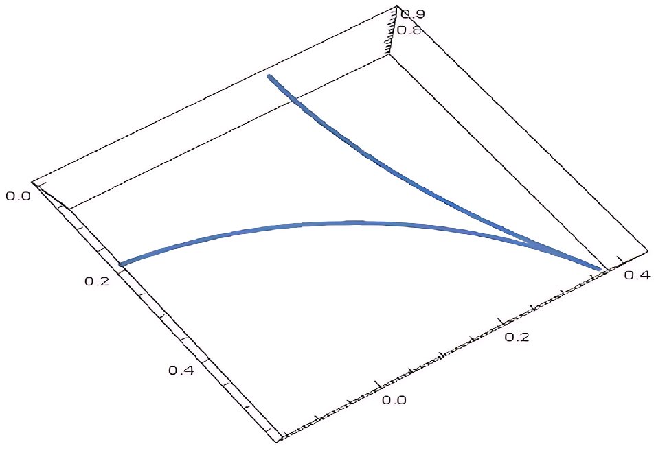
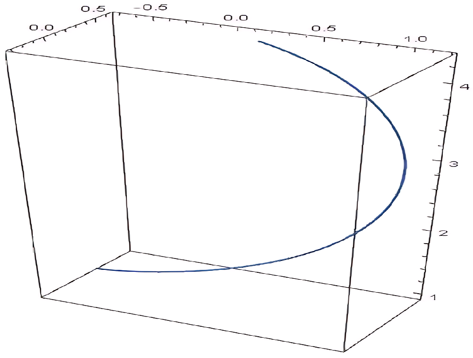
4. Electromagnetic Curves of $\mathcal{PLW}$ Along an Optical Fiber

The initial investigation by Poincaré, Lorentz, and Abraham into the flow of a charged point particle in flat spacetime has been highly popular in scientific studies. Thus, the electrodynamics of moving objects served as a springboard for the study of special relativity put forward by Einstein. Maxwell’s equations also served as a source of inspiration and direction for Poincare and Lorentz as they explored spacetime transformation. This offered development to the utmost unity of non-curved spacetime. Thus, it is accurate to say that Maxwell’s equations were crucial in understanding the deep relationship with the dynamics of the main physical influences and connections in this setting. Subsequent investigations ultimately resulted in integrating the electromagnetic field and spacetime geometry. Finally, it is noted that at the fundamental foundation of the electromagnetic field, the field equations are completely generic. One area of inquiry at the intersection of differential geometry and physics is the analysis of magnetic fields on a Riemannian manifold and the magnetic curves that accompany them.

On the Riemannian manifold, the magnetic field is characterized as a closed-2 form. The skew-symmetric one-to-one tensor defines the Lorentz force on R. These basic facts allow us to characterize a worldline or route generated with the help of the magnetic field as a space curve which is parameterized with arc-length on R if and only if it matches the Lorentz equation

$${\xi }_{vv}=\Phi {\xi }_v,$$

where $\xi =\xi \left(v\right)$ [35,36].

4.1. The Lie Reduction

Lie’s reduction refers to a method used in the study of Lie groups and Lie algebras, particularly aimed at simplifying the structure of complex systems. The process typically involves reducing a Lie group or Lie algebra to a simpler, often lower-dimensional model that retains essential properties. This simplification makes it easier to understand the group’s behavior and identify symmetries. In the context of Lie groups, Lie’s reduction is often applied to analyze their actions on manifolds, simplifying the study of continuous symmetries. The goal is to reduce the complexity of a given system while preserving key features, especially invariants or conserved quantities. Lie’s reduction also plays a crucial role in the study of integrable systems and quantum mechanics, where it can simplify the Hamiltonian or the equations of motion. Assume that $\alpha$ is a curve on G and $v:I\to TG$ is its $C^{\infty }$ lifting. Then, the Lie reduction of v is

$$\begin{array}{ccccc}V& :& I& \to & g\\ & & \left(t\right)& \to & V\left(t\right)={\left(d{L}_{{\alpha }^{-1}\left(t\right)}\right)}_{\alpha \left(t\right)}v\left(t\right),\end{array}$$

where, for $p\in G$ and $q\in g$, ${\left(d{L}_p\right)}_q$ is the derivative of $L_p$ at $q.$ In particular, the Lie reduction of ${\alpha }^{\prime }:I\to TG$ (or $\alpha$) corresponds to a smooth curve $T:I\to g$, which is defined by

$$T\left(t\right){\left(d{L}_{{\alpha }^{-1}\left(t\right)}\right)}_{\alpha \left(t\right)}\dot{\alpha }\left(t\right),$$

where $\dot{\alpha }\left(t\right)={\displaystyle \frac{d\alpha }{dt}}$. Let us assume that $v_0,v_1$ and $v_2$ are $C^{\infty }$ lifting of $\alpha .$ Then, it can be formulated as

$$\begin{array}{ccc}{\left(d{L}_{{\alpha }^{-1}\left(t\right)}\right)}_{\alpha \left(t\right)}{\nabla }_{{\displaystyle \frac{d}{dt}}{v}_0}& =& {\displaystyle \frac{d{V}_0}{dt}}+{\displaystyle \frac{1}{2}}[U,V_0]\\ {\left(d{L}_{{\alpha }^{-1}\left(t\right)}\right)}_{\alpha \left(t\right)}R\left(v_0,v_1\right)v_2& =& {\displaystyle \frac{1}{4}}[V_2,[V_0,V_1]],\end{array}$$

where $V_0,V_1,V_2$ are the Lie reduction of $v_0,v_1,v_2$ [37,38,39].

Let us assume that $\alpha$ is a curve on G, $\left\{t,n,b\right\}$ is its Frenet frame and $T,N,B$ are the Lie reduction of $t,n,b$, respectively. Now, we give the transformation function between $\omega$ and $\tilde{\omega }$, where $\omega$ and $\tilde{\omega }$ are a specific function that characterizes magnetic curves in association with the magnetic field [39].

$$\begin{array}{ccc}\hfill \tilde{\omega }& =& ⟨[{\left(d{L}_{{\alpha }^{-1}\left(s\right)}\right)}_{\alpha \left(s\right)}W,{\left(d{L}_{{\alpha }^{-1}\left(s\right)}\right)}_{\alpha \left(s\right)}n],{\left(d{L}_{{\alpha }^{-1}\left(s\right)}\right)}_{\alpha \left(s\right)}b⟩\hfill \\ & =& ⟨{\left(d{L}_{{\alpha }^{-1}\left(s\right)}\right)}_{\alpha \left(s\right)}[W,n],{\left(d{L}_{{\alpha }^{-1}\left(s\right)}\right)}_{\alpha \left(s\right)}b⟩\hfill \\ & =& ⟨[W,n],b⟩\hfill \\ & =& \omega .\hfill \end{array}$$

Let us consider again the curve $\alpha$, which is the conjugate pair of a curve $\beta$, and its RMF as $\left\{e_1,{\epsilon }_1,{\epsilon }_2\right\}.$ A new notation will be shown for the derivatives of RMF vectors as follows:

$$\begin{array}{ccc}\hfill {\nabla }_{{\displaystyle \frac{d}{ds}}}{e}_1& =& {\varkappa }_1{\epsilon }_1-{\varkappa }_2{\epsilon }_2,\hfill \\ \hfill {\nabla }_{{\displaystyle \frac{d}{ds}}}{\epsilon }_1& =& -{\varkappa }_1{e}_1,\hfill \\ \hfill {\nabla }_{{\displaystyle \frac{d}{ds}}}{\epsilon }_2& =& {\varkappa }_2{e}_1.\hfill \end{array}$$

(21)

The Lie reduction of the curve $\alpha$ corresponds to the differentiable curve $V:I\to g$. The Lie reduction of RMF $\left\{e_1,{\epsilon }_1,{\epsilon }_2\right\}$ can also be written as $\left\{E_1,{\mathcal{E}}_1,{\mathcal{E}}_2\right\}.$ In this case, one can write

$$\begin{array}{ccc}\hfill E_1& =& {\left(d{L}_{{\alpha }^{-1}}\right)}_{\alpha }{e}_1,\hfill \\ \hfill {\mathcal{E}}_1& =& {\left(d{L}_{{\alpha }^{-1}}\right)}_{\alpha }{\epsilon }_1,\hfill \\ \hfill {\mathcal{E}}_2& =& {\left(d{L}_{{\alpha }^{-1}}\right)}_{\alpha }{\epsilon }_2,\hfill \end{array}$$

Since the RMF is an orthonormal basis, the following equations can be written:

$$\begin{array}{ccc}\hfill ⟨e_1,e_1⟩& =& ⟨{\left(d{L}_{{\alpha }^{-1}}\right)}_{\alpha }{e}_1,{\left(d{L}_{{\alpha }^{-1}}\right)}_{\alpha }{e}_1⟩=⟨E_1,E_1⟩=1,\hfill \\ \hfill ⟨{\epsilon }_1,{\epsilon }_1⟩& =& ⟨{\left(d{L}_{{\alpha }^{-1}}\right)}_{\alpha }{\epsilon }_1,{\left(d{L}_{{\alpha }^{-1}}\right)}_{\alpha }{\epsilon }_1⟩=⟨{\mathcal{E}}_1,{\mathcal{E}}_1⟩=1,\hfill \\ \hfill ⟨{\epsilon }_2,{\epsilon }_2⟩& =& ⟨{\left(d{L}_{{\alpha }^{-1}}\right)}_{\alpha }{\epsilon }_2,{\left(d{L}_{{\alpha }^{-1}}\right)}_{\alpha }{\epsilon }_2⟩=⟨{\mathcal{E}}_2,{\mathcal{E}}_2⟩=1,\hfill \end{array}$$

and

$$\begin{array}{ccc}\hfill ⟨e_1,{\epsilon }_1⟩& =& ⟨{\left(d{L}_{{\alpha }^{-1}}\right)}_{\alpha }{e}_1,{\left(d{L}_{{\alpha }^{-1}}\right)}_{\alpha }{\epsilon }_1⟩=⟨E_1,{\mathcal{E}}_1⟩=0,\hfill \\ \hfill ⟨e_1,{\epsilon }_2⟩& =& ⟨{\left(d{L}_{{\alpha }^{-1}}\right)}_{\alpha }{e}_1,{\left(d{L}_{{\alpha }^{-1}}\right)}_{\alpha }{\epsilon }_2⟩=⟨E_1,{\mathcal{E}}_2⟩=0,\hfill \\ \hfill ⟨{\epsilon }_1,{\epsilon }_2⟩& =& ⟨{\left(d{L}_{{\alpha }^{-1}}\right)}_{\alpha }{\epsilon }_1,{\left(d{L}_{{\alpha }^{-1}}\right)}_{\alpha }{\epsilon }_2⟩=⟨{\mathcal{E}}_1,{\mathcal{E}}_2⟩=0.\hfill \end{array}$$

That is, $\left\{E_1,{\mathcal{E}}_1,{\mathcal{E}}_2\right\}$, which is the Lie reduction of $\left\{e_1,{\epsilon }_1,{\epsilon }_2\right\}$, is an orthonormal frame. Since the metric is left invariant, we can write

$$V={\left(d{L}_{{\alpha }^{-1}}\right)}_{\alpha }{\alpha }^{\prime }={\left(d{L}_{{\alpha }^{-1}}\right)}_{\alpha }{e}_1=E_1$$

and

$$∥V^{\prime }∥=\parallel {\left(d{L}_{{\alpha }^{-1}}\right)}_{\alpha }{\nabla }_{{\displaystyle \frac{d}{ds}}}{\alpha }^{\prime }\parallel =\parallel {\nabla }_{{\displaystyle \frac{d}{ds}}}{\alpha }^{\prime }\parallel ={\varkappa }_1^2+{\varkappa }_2^2.$$

Theorem 1.

Let us assume that the curve α is the conjugate pair of a curve β, and $\left\{e_1,{\epsilon }_1,{\epsilon }_2\right\}$ is its RMF. If $\left\{E_1,{\mathcal{E}}_1,{\mathcal{E}}_2\right\}$ is the Lie reduction of $\left\{e_1,{\epsilon }_1,{\epsilon }_2\right\}$ then

$$\begin{array}{ccc}\hfill E_1^{\prime }& =& {\varkappa }_1{\mathcal{E}}_1-{\varkappa }_2{\mathcal{E}}_2,\hfill \\ \hfill {\mathcal{E}}_1^{\prime }& =& -{\varkappa }_1{E}_1-{\tilde{\tau }}_G{\mathcal{E}}_2,\hfill \\ \hfill {\mathcal{E}}_2^{\prime }& =& {\varkappa }_2{E}_1+{\tilde{\tau }}_G{\mathcal{E}}_1,\hfill \end{array}$$

where ${\tilde{\tau }}_G={\displaystyle \frac{1}{2}}⟨\left[E_1,{\mathcal{E}}_1\right],{\mathcal{E}}_2⟩.$

Proof. 

Considering the Equations (1) and (21) with the left invariant metric, we obtain the following results:

$$\begin{array}{ccc}\hfill -{\varkappa }_1& =& ⟨{\nabla }_{{\displaystyle \frac{d}{ds}}}{\epsilon }_1,e_1⟩\hfill \\ & =& ⟨{\left(d{L}_{{\alpha }^{-1}}\right)}_{\alpha }{\nabla }_{{\displaystyle \frac{d}{ds}}}{\epsilon }_1,{\left(d{L}_{{\alpha }^{-1}}\right)}_{\alpha }{e}_1⟩\hfill \\ & =& ⟨{\mathcal{E}}_1^{\prime }+{\displaystyle \frac{1}{2}}\left[V,{\mathcal{E}}_1\right],E_1⟩\hfill \\ & =& ⟨{\mathcal{E}}_1^{\prime },E_1⟩+{\displaystyle \frac{1}{2}}⟨\left[V,{\mathcal{E}}_1\right],E_1⟩\hfill \\ & =& ⟨{\mathcal{E}}_1^{\prime },E_1⟩\hfill \end{array}$$

(22)

and

$$\begin{array}{ccc}\hfill {\left(d{L}_{{\alpha }^{-1}}\right)}_{\alpha }{\nabla }_{{\displaystyle \frac{d}{ds}}}{\epsilon }_1& =& {\mathcal{E}}_1^{\prime }+{\displaystyle \frac{1}{2}}\left[V,{\mathcal{E}}_1\right]\hfill \\ & =& {\mathcal{E}}_1^{\prime }+{\displaystyle \frac{1}{2}}⟨\left[V,{\mathcal{E}}_1\right],{\mathcal{E}}_2⟩{\mathcal{E}}_2\hfill \\ & =& {\mathcal{E}}_1^{\prime }+{\tilde{\tau }}_G{\mathcal{E}}_2.\hfill \end{array}$$

(23)

When (22) and (23) are considered together, we obtain

$${\mathcal{E}}_1^{\prime }=-{\varkappa }_1{E}_1-{\tilde{\tau }}_G{\mathcal{E}}_2.$$

By making similar calculations, we obtain

$${\mathcal{E}}_2^{\prime }={\varkappa }_2{E}_1.$$

Taking into consideration Equations (1) and (21), we have

$${\left(d{L}_{{\alpha }^{-1}}\right)}_{\alpha }{\nabla }_{{\displaystyle \frac{d}{ds}}}{\alpha }^{\prime }={\left(d{L}_{{\alpha }^{-1}}\right)}_{\alpha }{\nabla }_{{\displaystyle \frac{d}{ds}}}{e}_1,$$

and

$$E_1^{\prime }={\varkappa }_1{\mathcal{E}}_1-{\varkappa }_2{\mathcal{E}}_2.$$

□

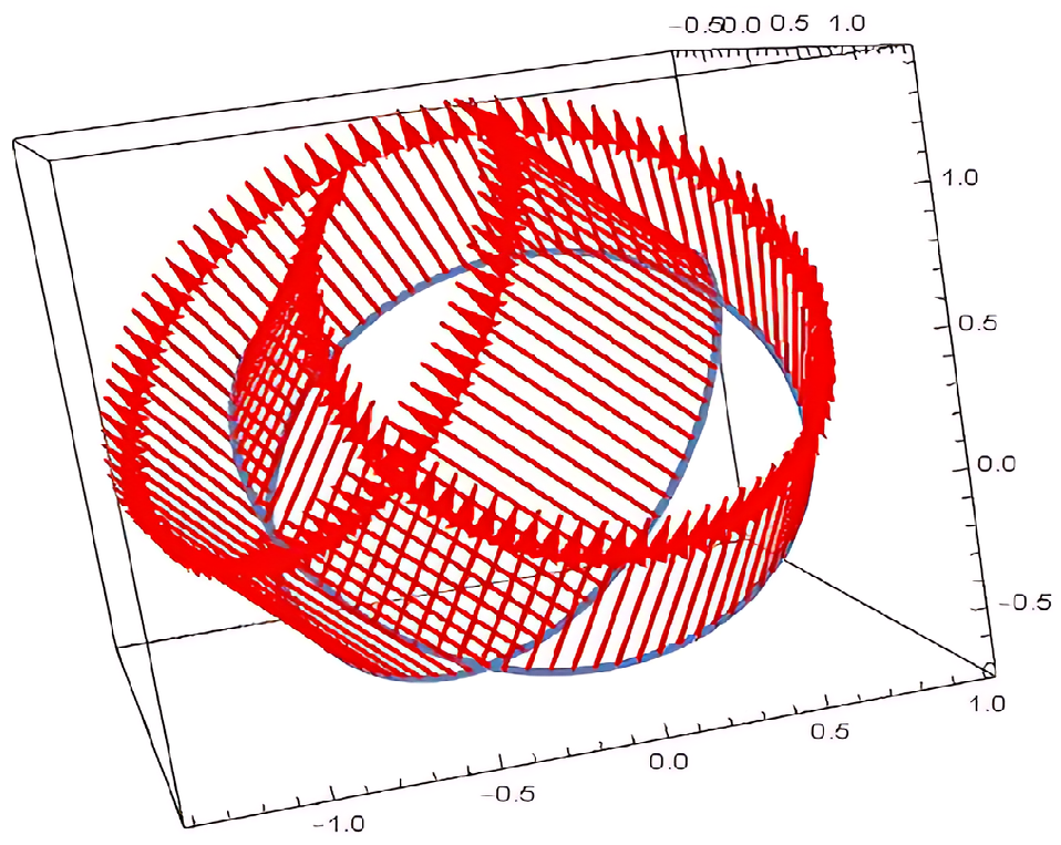
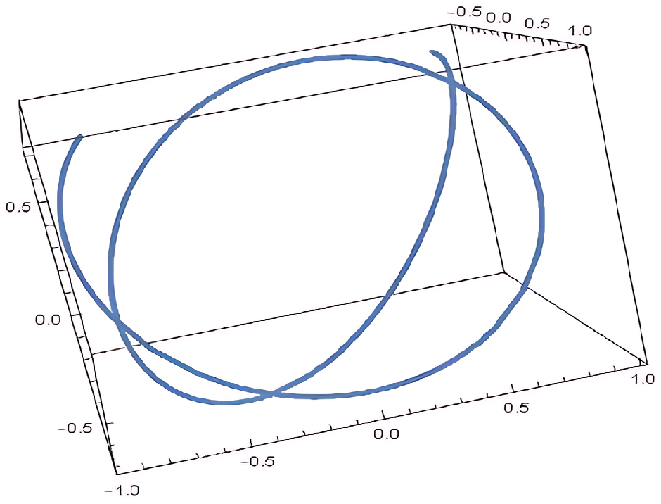
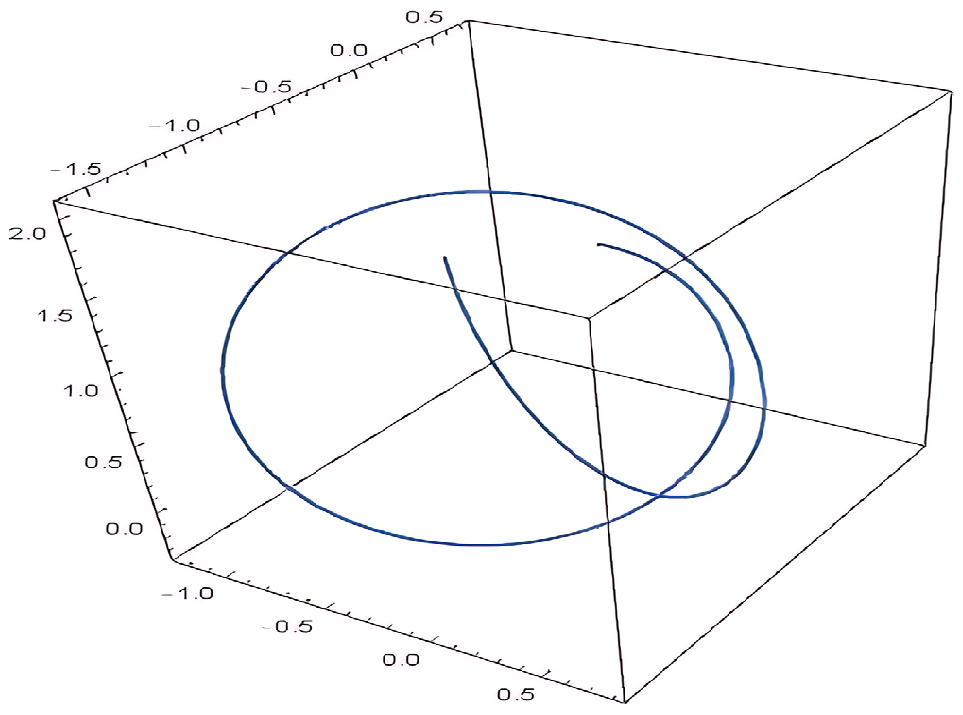
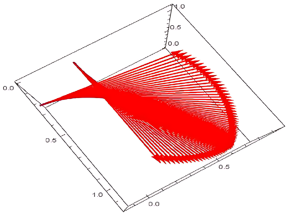
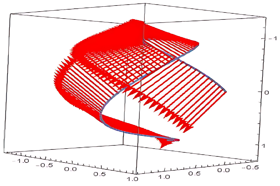
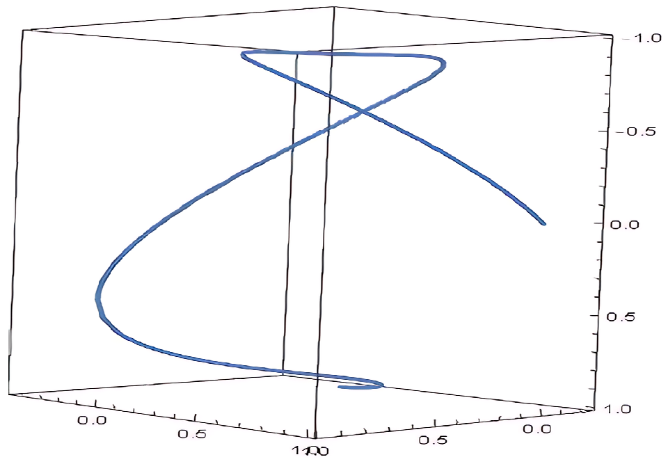
4.2. Magnetic Trajectories of Electromagnetic Curves

In the case that $\mathfrak{N}\perp e_1$, we can suppose that $\mathfrak{M}$ is an optical fiber that is referred to as $\alpha$ existing in a Lie group where a $\mathcal{PLW}$ linearly spreads across into an optical fiber. The $\mathfrak{N}$ in an optical fiber refers to the direction of the case of linear $\mathcal{PLW}$. When this situation happens, we presume that $\mathfrak{N}$ is on a plane which is perpendicular to $e_1$ across the space curve $\alpha$.

In three-dimensional Lie group G, let $\zeta \in \chi \left(G\right)$ be vector field ($div$$\zeta =0$) and for ${\xi }_1,{\xi }_2,{\xi }_3\in \chi \left(G\right)$, the Lie bracket is

$$⟨[{\xi }_1,{\xi }_2],{\xi }_3⟩={\Pi }_3\left({\xi }_1,{\xi }_2,{\xi }_3\right),$$

where ${\Pi }_3$ is volume three forms of G. Then, the Lorentz force is formulated as

$$\begin{array}{ccc}\hfill ⟨\Phi \left({\xi }_1\right),{\xi }_2⟩& =& \mathfrak{F}\left({\xi }_1,{\xi }_2\right)=\left(i_{\zeta }{\Pi }_3\right)\left({\xi }_1,{\xi }_2\right)\hfill \\ & =& {\Pi }_3\left(\zeta ,{\xi }_1,{\xi }_2\right)\hfill \\ & =& ⟨[\zeta ,{\xi }_1],{\xi }_2⟩,\hfill \end{array}$$

where $\mathfrak{F}=i_{\zeta }{\Pi }_3$ is a magnetic field. Taking the last equality into account, we can write the following equation:

$$\Phi \left({\xi }_1\right)=[\zeta ,{\xi }_1].$$

Then, the Lorentz equation is

$$\Phi \left({\xi }_1\right)={\xi }_1^{\prime }=[\zeta ,{\xi }_1].$$

(24)

Now, let us consider the equation obtained in (4). The derivative equation for the electric field $\mathfrak{N}$ is

$${\mathfrak{N}}^{\prime }=\left(-{\varkappa }_1⟨\mathfrak{N},{\epsilon }_1⟩+{\varkappa }_2⟨\mathfrak{N},{\epsilon }_2⟩\right)e_1+\mathfrak{l}⟨\mathfrak{N},{\epsilon }_2⟩{\epsilon }_1-\mathfrak{l}⟨\mathfrak{N},{\epsilon }_1⟩{\epsilon }_2.$$

Given the assumptions in Equation (24) and the identity below

$$⟨\Phi \left(\mathfrak{N}\right),e_1⟩=-⟨\mathfrak{N},\Phi \left(e_1\right)⟩,$$

the Lorentz forces for the electric field $\mathfrak{N}$ of magnetic field $\mathfrak{F}$ are

$$\begin{array}{ccc}\hfill \Phi \left(e_1\right)& =& {\varkappa }_1{\epsilon }_1-{\varkappa }_2{\epsilon }_2,\hfill \\ \hfill \Phi \left({\epsilon }_1\right)& =& -{\varkappa }_1{e}_1-\mathfrak{l}{\epsilon }_2,\hfill \\ \hfill \Phi \left({\epsilon }_2\right)& =& {\varkappa }_2{e}_1+\mathfrak{l}{\epsilon }_1.\hfill \end{array}$$

The magnetic field $\mathfrak{F}$ is easy to find, represented by the following equation:

$$\mathfrak{F}=-\mathfrak{l}{e}_1+{\varkappa }_2{\epsilon }_1+{\varkappa }_1{\epsilon }_2.$$

Assuming that $e_1$ is moved in parallel, since $\mathfrak{l}=0$, the magnetic vector field is

$$\mathfrak{F}={\varkappa }_2{\epsilon }_1+{\varkappa }_1{\epsilon }_2$$

and the Lorentz forces of the $RMF$ of the magnetic curve can be given by

$$\left(\begin{array}{c}\Phi \left(e_1\right)\\ \Phi \left({\epsilon }_1\right)\\ \Phi \left({\epsilon }_2\right)\end{array}\right)=\left(\begin{array}{ccc}0& {\varkappa }_1& -{\varkappa }_2\\ -{\varkappa }_1& 0& 0\\ {\varkappa }_2& 0& 0\end{array}\right)\left(\begin{array}{c}{e}_1\\ {\epsilon }_1\\ {\epsilon }_2\end{array}\right).$$

Let us assume that the curve $\alpha$ is the conjugate pair of a curve $\beta$, $\{e_1,{\epsilon }_1,{\epsilon }_2\}$ is its RMF, and $\{E_1,{\mathcal{E}}_1,{\mathcal{E}}_2\}$ is the Lie reduction of $\{e_1,{\epsilon }_1,{\epsilon }_2\}$. Also, let $\tilde{\mathfrak{F}}$ be the Lie reduction of magnetic field $\mathfrak{F}.$ Using Equation (24), one can write

$$\Phi \left({\mathcal{E}}_1\right)=\left[\tilde{\mathfrak{F}},{\mathcal{E}}_1\right].$$

(25)

Using Equation (25), and with the help of simple calculations,

$$\begin{array}{ccc}\hfill ⟨\Phi \left({\mathcal{E}}_1\right),E_1⟩& =& ⟨\left[\tilde{\mathfrak{F}},{\mathcal{E}}_1\right],E_1⟩\hfill \\ & =& -⟨\Phi \left(E_1\right),{\mathcal{E}}_1⟩\hfill \\ & =& -{\varkappa }_1,\hfill \\ \hfill ⟨\Phi \left({\mathcal{E}}_1\right),{\mathcal{E}}_1⟩& =& 0,\hfill \\ \hfill ⟨\Phi \left({\mathcal{E}}_1\right),{\mathcal{E}}_2⟩& =& -\tilde{\mathfrak{l}}.\hfill \end{array}$$

Then, the Lorentz force $\Phi \left({\mathcal{E}}_1\right)$ for the electric field $\mathfrak{N}$ can be written as:

$$\Phi \left({\mathcal{E}}_1\right)=-{\varkappa }_1{E}_1-\tilde{\mathfrak{l}}{\mathcal{E}}_2.$$

(26)

By repeating the same operations in (26), we have

$$\begin{array}{ccc}\hfill \Phi \left(E_1\right)& =& {\varkappa }_1{\mathcal{E}}_1-{\varkappa }_2{\mathcal{E}}_2,\hfill \\ \hfill \Phi \left({\mathcal{E}}_2\right)& =& {\varkappa }_2{E}_1+\tilde{\mathfrak{l}}{\mathcal{E}}_1,\hfill \end{array}$$

(27)

where $\tilde{\mathfrak{l}}=⟨\Phi \left({\mathcal{E}}_2\right),{\mathcal{E}}_1⟩.$ We give the transformation function between $\mathfrak{l}$ and $\tilde{\mathfrak{l}}$, where $\mathfrak{l}$ and $\tilde{\mathfrak{l}}$ are specific functions that characterize magnetic curves in association with the magnetic field.

$$\begin{array}{ccc}\hfill \tilde{\mathfrak{l}}& =& ⟨[{\left(d{L}_{{\alpha }^{-1}}\right)}_{\alpha }\mathfrak{F},{\left(d{L}_{{\alpha }^{-1}}\right)}_{\alpha }{\epsilon }_1],{\left(d{L}_{{\alpha }^{-1}}\right)}_{\alpha }{\epsilon }_2⟩\hfill \\ & =& ⟨{\left(d{L}_{{\alpha }^{-1}}\right)}_{\alpha }[\mathfrak{F},{\epsilon }_1],{\left(d{L}_{{\alpha }^{-1}\left(t\right)}\right)}_{\alpha \left(t\right)}{\epsilon }_2⟩\hfill \\ & =& ⟨[\mathfrak{F},{\epsilon }_1],{\epsilon }_2⟩\hfill \\ & =& \mathfrak{l}.\hfill \end{array}$$

In (5), since we assume that $e_1$ is parallel transported, $\mathfrak{l}=0$. That is, $\tilde{\mathfrak{l}}=0.$

Now, let us consider again the magnetic curve $\mathfrak{F}$ and its Lie reduction $\tilde{\mathfrak{F}}$. If we show the Lie reduction $\tilde{\mathfrak{F}}$ of the magnetic curve $\mathfrak{F}$ as

$$\tilde{\mathfrak{F}}=a_1{E}_1+a_2{\mathcal{E}}_1+a_3{\mathcal{E}}_2.$$

With the help of (25) and (27), we have

$$a_1=0,a_2={\displaystyle \frac{{\varkappa }_2}{{\tilde{\tau }}_G}}\mathrm{and}{a}_3={\displaystyle \frac{{\varkappa }_1}{{\tilde{\tau }}_G}}.$$

Therefore, $\tilde{\mathfrak{F}}$ can be written along V as

$$\tilde{\mathfrak{F}}={\displaystyle \frac{1}{{\tilde{\tau }}_G}}\left({\varkappa }_2{\mathcal{E}}_1+{\varkappa }_1{\mathcal{E}}_2\right).$$

In the case that $\mathfrak{N}\perp {\epsilon }_1$, we can suppose that $\mathfrak{M}$ is an optical fiber that is referred to as $\alpha$ existing in the Lie group where the $\mathcal{PLW}$ linearly spreads across into an optical fiber. The $\mathfrak{N}$ in an optical fiber refers to the direction of the case of linear $\mathcal{PLW}$. When this situation happens, we presume $\mathfrak{N}$ is on a plane which is perpendicular to ${\epsilon }_1$ across the space curve $\alpha$.

Let us consider the equation obtained in (10). The derivative equation for the electric field $\mathfrak{N}$ is

$${\mathfrak{N}}^{\prime }=\mathfrak{l}⟨\mathfrak{N},{\epsilon }_2⟩e_1+{\varkappa }_1⟨\mathfrak{N},e_1⟩{\epsilon }_1-\mathfrak{l}⟨\mathfrak{N},e_1⟩{\epsilon }_2.$$

Given the assumptions in Equation (24) and the identity below,

$$⟨\Phi \left(\mathfrak{N}\right),{\epsilon }_1⟩=-⟨\mathfrak{N},\Phi \left({\epsilon }_1\right)⟩.$$

the Lorentz forces for the electric field $\mathfrak{N}$ of magnetic field $\mathfrak{F}$ are

$$\begin{array}{ccc}\hfill \Phi \left(e_1\right)& =& {\varkappa }_1{\epsilon }_1-\mathfrak{l}{\epsilon }_2,\hfill \\ \hfill \Phi \left({\epsilon }_1\right)& =& -{\varkappa }_1{e}_1,\hfill \\ \hfill \Phi \left({\epsilon }_2\right)& =& \mathfrak{l}{e}_1.\hfill \end{array}$$

The magnetic field $\mathfrak{F}$ is

$$\mathfrak{F}=\mathfrak{l}{\epsilon }_1+{\varkappa }_1{\epsilon }_2.$$

Let us assume that ${\epsilon }_1$ is moved in parallel; since $\mathfrak{l}=0$, the magnetic vector field is

$$\mathfrak{F}={\varkappa }_1{\epsilon }_2,$$

and the Lorentz forces of the $RMF$ of the magnetic curve can be given by

$$\left(\begin{array}{c}\Phi \left(e_1\right)\\ \Phi \left({\epsilon }_1\right)\\ \Phi \left({\epsilon }_2\right)\end{array}\right)=\left(\begin{array}{ccc}0& {\varkappa }_1& 0\\ -{\varkappa }_1& 0& 0\\ 0& 0& 0\end{array}\right)\left(\begin{array}{c}{e}_1\\ {\epsilon }_1\\ {\epsilon }_2\end{array}\right).$$

Let us assume that $\tilde{\mathfrak{F}}$ is the Lie reduction of magnetic field $\mathfrak{F}.$ Using Equation (24), one can write

$$\Phi \left(E_1\right)=\left[\tilde{\mathfrak{F}},E_1\right].$$

(28)

Using Equation (28), and with the help of simple calculations,

$$\begin{array}{ccc}\hfill ⟨\Phi \left(E_1\right),E_1⟩& =& 0,\hfill \\ \hfill ⟨\Phi \left(E_1\right),{\mathcal{E}}_1⟩& =& ⟨\left[\tilde{\mathfrak{F}},E_1\right],{\mathcal{E}}_1⟩\hfill \\ & =& {\varkappa }_1,\hfill \\ \hfill ⟨\Phi \left(E_1\right),{\mathcal{E}}_2⟩& =& -\tilde{\mathfrak{l}}.\hfill \end{array}$$

Then, the Lorentz force $\Phi \left(E_1\right)$ for the electric field $\mathfrak{N}$ can be written as

$$\Phi \left(E_1\right)={\varkappa }_1{\mathcal{E}}_1-\tilde{\mathfrak{l}}{\mathcal{E}}_2.$$

(29)

By repeating the same operations in (29), we have

$$\begin{array}{ccc}\hfill \Phi \left({\mathcal{E}}_1\right)& =& -{\varkappa }_1{E}_1-{\tilde{\tau }}_G{\mathcal{E}}_2,\hfill \\ \hfill \Phi \left({\mathcal{E}}_2\right)& =& \tilde{\mathfrak{l}}{E}_1+{\tilde{\tau }}_G{\mathcal{E}}_1,\hfill \end{array}$$

(30)

where $\tilde{\mathfrak{l}}=⟨\Phi \left({\mathcal{E}}_2\right),E_1⟩.$ Since we assume that ${\epsilon }_1$ is parallel transported, $\mathfrak{l}=0$. That is, $\tilde{\mathfrak{l}}=0.$ If we show the Lie reduction $\tilde{\mathfrak{F}}$ of the magnetic curve $\mathfrak{F}$ as

$$\tilde{\mathfrak{F}}=a_1{E}_1+a_2{\mathcal{E}}_1+a_3{\mathcal{E}}_2.$$

With the help of (28) and (30), we have

$$a_1=-1,a_2=0\mathrm{and}{a}_3={\displaystyle \frac{{\varkappa }_1}{{\tilde{\tau }}_G}}.$$

Therefore, $\tilde{\mathfrak{F}}$ can be written along V as

$$\tilde{\mathfrak{F}}=-E_1+{\displaystyle \frac{{\varkappa }_1}{{\tilde{\tau }}_G}}{\mathcal{E}}_2.$$

In the case that $\mathfrak{N}\perp {\epsilon }_2$, we can suppose that $\mathfrak{M}$ is an optical fiber that is referred to as $\alpha$ existing in the Lie group where the $\mathcal{PLW}$ linearly spreads across into an optical fiber. The $\mathfrak{N}$ in an optical fiber refers to the direction of the case of linear $\mathcal{PLW}$. When this situation happens, we presume $\mathfrak{N}$ is on a plane which is perpendicular to ${\epsilon }_2$ across the space curve $\alpha$.

Let us consider the equation obtained in the Equation (16). The derivative equation for the electric field $\mathfrak{N}$ is

$${\mathfrak{N}}^{\prime }=\mathfrak{l}⟨\mathfrak{N},{\epsilon }_1⟩e_1-\mathfrak{l}⟨\mathfrak{N},e_1⟩{\epsilon }_1-{\varkappa }_2⟨\mathfrak{N},e_1⟩{\epsilon }_2.$$

Given the assumptions in Equation (24) and the identity below,

$$⟨\Phi \left(\mathfrak{N}\right),{\epsilon }_2⟩=-⟨\mathfrak{N},\Phi \left({\epsilon }_2\right)⟩,$$

the Lorentz forces for the electric field $\mathfrak{N}$ of magnetic field $\mathfrak{F}$ are

$$\begin{array}{ccc}\hfill \Phi \left(e_1\right)& =& -\mathfrak{l}{\epsilon }_1-{\varkappa }_2{\epsilon }_2,\hfill \\ \hfill \Phi \left({\epsilon }_1\right)& =& \mathfrak{l}{e}_1,\hfill \\ \hfill \Phi \left({\epsilon }_2\right)& =& {\varkappa }_2{e}_1.\hfill \end{array}$$

The magnetic field $\mathfrak{F}$ is

$$\mathfrak{F}={\varkappa }_2{\epsilon }_1-\mathfrak{l}{\epsilon }_2.$$

Considering that ${\epsilon }_2$ is moved in parallel, since $\mathfrak{l}=0$, the magnetic vector field is

$$\mathfrak{F}={\varkappa }_2{\epsilon }_1$$

and the Lorentz forces of the $RMF$ of magnetic curve can be given by

$$\left(\begin{array}{c}\Phi \left(e_1\right)\\ \Phi \left({\epsilon }_1\right)\\ \Phi \left({\epsilon }_2\right)\end{array}\right)=\left(\begin{array}{ccc}0& 0& -{\varkappa }_2\\ 0& 0& 0\\ {\varkappa }_2& 0& 0\end{array}\right)\left(\begin{array}{c}{e}_1\\ {\epsilon }_1\\ {\epsilon }_2\end{array}\right).$$

Let us assume that $\tilde{\mathfrak{F}}$ is the Lie reduction of magnetic field $\mathfrak{F}.$ Using Equation (24), one can write

$$\Phi \left({\mathcal{E}}_1\right)=\left[\tilde{\mathfrak{F}},{\mathcal{E}}_1\right].$$

(31)

Using Equation (31), and with the help of simple calculations,

$$\begin{array}{ccc}\hfill ⟨\Phi \left({\mathcal{E}}_1\right),E_1⟩& =& \tilde{\mathfrak{l}},\hfill \\ \hfill ⟨\Phi \left({\mathcal{E}}_1\right),{\mathcal{E}}_1⟩& =& 0\hfill \\ \hfill ⟨\Phi \left({\mathcal{E}}_1\right),{\mathcal{E}}_2⟩& =& -⟨\left[\tilde{\mathfrak{F}},{\mathcal{E}}_1\right],{\mathcal{E}}_2⟩\hfill \\ & =& {\tilde{\tau }}_G.\hfill \end{array}$$

Then, the Lorentz force $\Phi \left({\mathcal{E}}_1\right)$ for the electric field $\mathfrak{N}$ can be written as

$$\Phi \left({\mathcal{E}}_1\right)=\tilde{\mathfrak{l}}{E}_1+{\tilde{\tau }}_G{\mathcal{E}}_2.$$

(32)

By repeating the same operations in (32), we have

$$\begin{array}{ccc}\hfill \Phi \left(E_1\right)& =& -\tilde{\mathfrak{l}}{\mathcal{E}}_1-{\varkappa }_2{\mathcal{E}}_2,\hfill \\ \hfill \Phi \left({\mathcal{E}}_2\right)& =& {\varkappa }_2{E}_1+{\tilde{\tau }}_G{\mathcal{E}}_1,\hfill \end{array}$$

(33)

where $\tilde{\mathfrak{l}}=⟨\Phi \left({\mathcal{E}}_1\right),E_1⟩.$ Since we assume that ${\epsilon }_2$ is parallel transported, $\mathfrak{l}=0$. That is, $\tilde{\mathfrak{l}}=0.$ If we show the Lie reduction $\tilde{\mathfrak{F}}$ of the magnetic curve $\mathfrak{F}$ as

$$\tilde{\mathfrak{F}}=a_1{E}_1+a_2{\mathcal{E}}_1+a_3{\mathcal{E}}_2.$$

With the help of (31) and (33), we have

$$a_1=1,a_2={\displaystyle \frac{{\varkappa }_2}{{\tilde{\tau }}_G}}\mathrm{and}{a}_3=0.$$

Therefore, $\tilde{\mathfrak{F}}$ can be written along V as

$$\tilde{\mathfrak{F}}=E_1+{\displaystyle \frac{{\varkappa }_1}{{\tilde{\tau }}_G}}{\mathcal{E}}_1.$$

5. Discussion and Conclusions

The construction of a Berry phase for a $\mathcal{PLW}$ along an optical fiber, known as a space curve or electromagnetic curve, is studied in depth, not only physically but also geometrically. In the world of differential geometry, space curves are usually defined and considered as a regular curve. This article studies the detailed situations of an optical fiber’s geometric phase and the electromagnetic curve with a conjugate curve model. With this model, unnecessary bending around the tangent was prevented and a more dynamic characterization was obtained that can be worked on even if the second derivative of the curve is zero. The purpose for doing this is just because the expectations of our study helps the reader while reading this article. Moreover, we set a link from the Rytov parallel transportation law to Fermi–Walker transportation for a $\mathcal{PLW}$ which is linearly spreading into an optical fiber. The link that we set between these transportation rules creates the energy of the electric field, which is named $\mathfrak{N}$.

References

- Comtet, A. On the Landau levels on the hyperbolic plane. Ann. Phys. 1987, 173, 185–209. [Google Scholar] [CrossRef]
- Druţă-Romaniuc, S.L.; Munteanu, M.I. Killing magnetic curves in a Minkowski 3-space. Nonlinear Anal. Real World Appl. 2013, 14, 383–396. [Google Scholar] [CrossRef]
- Efimov, D.I. The magnetic geodesic flow on a homogeneous symplectic manifold. Sib. Math. J. 2005, 46, 83–93. [Google Scholar] [CrossRef]
- Munteanu, M.I.; Nistor, A.I. The classification of Killing magnetic curves in S2 × . J. Geom. Phys. 2012, 62, 170–182. [Google Scholar] [CrossRef]
- Novikov, S.P. The Hamiltonian formalism and a many-valued analogue of Morse theory. Russ. Math. Surv. 1982, 37, 1. [Google Scholar] [CrossRef]
- Yazıcı, B.D.; Okuyucu, O.Z.; Tosun, M. Framed curves in three-dimensional Lie groups and a Berry phase model. J. Geom. Phys. 2022, 182, 104682. [Google Scholar] [CrossRef]
- Sunada, T. Magnetic flows on a Riemannian surface. In Proceedings of the KAIST Mathematics Workshop Analysis and Geometry, Taejeon, Republic of Korea, 3–6 January 1993; Volume 8, pp. 93–108. [Google Scholar]
- Körpinar, T. Bianchi type-I cosmological models for inextensible flows of biharmonic particles by using curvature tensor field in spacetime. Int. J. Theor. Phys. 2015, 54, 1762–1774. [Google Scholar] [CrossRef]
- Özdemir, Z. A new calculus for the treatment of Rytov’s law in the optical fiber. Optik 2020, 216, 164892. [Google Scholar] [CrossRef]
- Gürbüz, N.E. The pseudo-null geometric phase along optical fiber. Int. J. Geom. Methods Mod. Phys. 2021, 18, 2150230. [Google Scholar] [CrossRef]
- Gürbüz, N.E. The variation of the electric field along optic fiber for null Cartan and pseudo-null frames. Int. J. Geom. Methods Mod. Phys. 2021, 18, 2150122. [Google Scholar] [CrossRef]
- Gürbüz, N.E. The null geometric phase along optical fiber for anholonomic coordinates. Optik 2022, 258, 168841. [Google Scholar] [CrossRef]
- Berry, M.V. The adiabatic phase and Pancharatnam’s phase for polarized light. J. Mod. Opt. 1987, 34, 1401–1407. [Google Scholar] [CrossRef]
- Nurkan, S.K.; Ceyhan, H.; Özdemir, Z.; Gök, İ. Electromagnetic curves and Rytov’s law in the optical fiber with Maxwellian evolution via alternative moving frame. Rev. Mex. Fís. 2023, 69, 061301-1. [Google Scholar] [CrossRef]
- Körpinar, T.; Demirkol, R.C. Electromagnetic curves of the linearly polarized light wave along an optical fiber in a 3D Riemannian manifold with Bishop equations. Optik 2020, 200, 163334. [Google Scholar] [CrossRef]
- Körpinar, T.; Demirkol, R.C. Berry phase of the linearly polarized light wave along an optical fiber and its electromagnetic curves via quasi adapted frame. Waves Random Complex Media 2022, 32, 1497–1516. [Google Scholar] [CrossRef]
- Kugler, M.; Shtrikman, S. Berry’s phase, locally inertial frames, and classical analogues. Phys. Rev. D 1988, 37, 934. [Google Scholar] [CrossRef]
- Ross, J.N. The rotation of the polarization in low birefringence monomode optical fibres due to geometric effects. Opt. Quantum Electron. 1984, 16, 455–461. [Google Scholar] [CrossRef]
- Ceyhan, H.; Özdemir, Z.; Gök, İ.; Ekmekci, F.N. Electromagnetic curves and rotation of the polarization plane through alternative moving frame. Eur. Phys. J. Plus 2020, 135, 867. [Google Scholar] [CrossRef]
- Casas-Alvero, E. Singularities of Plane Curves; Cambridge University Press: Cambridge, UK, 2000. [Google Scholar]
- El Kahoui, M.H.; Moussa, Z.Y. An algorithm to compute the adjoint ideal of an affine plane algebraic curve. Math. Comput. Sci. 2014, 8, 289–298. [Google Scholar] [CrossRef]
- Gorenstein, D. An arithmetic theory of adjoint plane curves. Trans. Am. Math. Soc. 1952, 72, 414–436. [Google Scholar] [CrossRef]
- Zymaris, A.S.; Papadimitriou, D.I.; Giannakoglou, K.C.; Othmer, C. Adjoint wall functions: A new concept for use in aerodynamic shape optimization. J. Comput. Phys. 2010, 229, 5228–5245. [Google Scholar] [CrossRef]
- Hunt, B. Differential Geometry, Curves–Surfaces–Manifolds; AMS: Providence, RI, USA, 2006. [Google Scholar]
- Nurkan, S.K.; Güven, İ.A.; Karacan, M.K. Characterizations of adjoint curves in Euclidean 3-space. Sect. A Phys. Sci. 2019, 89, 155–161. [Google Scholar] [CrossRef]
- Sariaydin, M.T.; Korpinar, T. An Approach for Vectorial Moments in Euclidean 3-Space. Honam Math. J. 2020, 42, 187–195. [Google Scholar]
- Güler, F. Surface Pencil with a Common Timelike Adjoint Curve. Palest. J. Math. 2024, 13, 302–309. [Google Scholar]
- Güler, F. Construction of surface pencil with a given spacelike adjoint curve. Adv. Stud. Euro-Tbil. Math. J. 2022, 15, 1–11. [Google Scholar] [CrossRef]
- Crouch, P.; Leite, F.S. The dynamic interpolation problem: On Riemannian manifolds, Lie groups, and symmetric spaces. J. Dyn. Control. Syst. 1995, 1, 177–202. [Google Scholar] [CrossRef]
- Al-Jedani, A.; Abdel-Baky, R. Sweeping surfaces due to conjugate Bishop frame in 3-dimensional Lie group. Symmetry 2023, 15, 910. [Google Scholar] [CrossRef]
- Keskin, Ö.; Yaylı, Y. Normal Fermi-walker derivative. Math. Sci. Appl. E-Notes 2017, 5, 1–8. [Google Scholar] [CrossRef]
- Karakuş, F.; Yayli, Y. The Fermi–Walker derivative in Lie groups. Int. J. Geom. Methods Mod. Phys. 2013, 10, 1320011. [Google Scholar] [CrossRef]
- Markovski, B.; Vinitsky, S.I. Topological Phases in Quantum Theory; World Scientific: Dubna, Russia, 1989. [Google Scholar]
- Kravtsov, Y.A.; Orlov, Y.I. Geometrical Optics of Inhomogeneous Media; Springer: Berlin/Heidelberg, Germany, 1990. [Google Scholar]
- Munteanu, M.I. Magnetic curves in a Euclidean space: One example, several approaches. Publ. de L’Inst. Math. 2013, 94, 141–150. [Google Scholar] [CrossRef]
- Barros, M.; Cabrerizo, J.L.; Fernández, M.; Romero, A. Magnetic vortex filament flows. J. Math. Phys. 2007, 48, 082904. [Google Scholar] [CrossRef]
- Noakes, L. Null cubics and Lie quadratics. J. Math. Phys. 2003, 44, 1436–1448. [Google Scholar] [CrossRef]
- Popiel, T.; Noakes, L. Elastica in SO3. J. Aust. Math. Soc. 2007, 83, 105–124. [Google Scholar] [CrossRef]
- Turhan, T. Magnetic trajectories in three-dimensional Lie groups. Math. Methods Appl. Sci. 2020, 43, 2747–2758. [Google Scholar] [CrossRef]
Disclaimer/Publisher’s Note: The statements, opinions and data contained in all publications are solely those of the individual author(s) and contributor(s) and not of MDPI and/or the editor(s). MDPI and/or the editor(s) disclaim responsibility for any injury to people or property resulting from any ideas, methods, instructions or products referred to in the content. |
© 2024 by the author. Licensee MDPI, Basel, Switzerland. This article is an open access article distributed under the terms and conditions of the Creative Commons Attribution (CC BY) license (https://creativecommons.org/licenses/by/4.0/).