Phase Portraits and Abundant Soliton Solutions of a Hirota Equation with Higher-Order Dispersion

Abstract

The Hirota equation, an advanced variant of the nonlinear Schrödinger equation with cubic nonlinearity, incorporates time-delay adjustments and higher-order dispersion terms, offering an enhanced approximation for wave propagation in optical fibers and oceanic systems. By utilizing the traveling wave transformation generated from Lie point symmetry analysis with the combination of generalized exponential differential rational function and modified Bernoulli sub-ODE techniques, several traveling wave solutions, such as periodic, singular-periodic, and kink solitons, emerge. To examine the solutions visually, parametric values are adjusted to create 3D, contour, and 2D illustrations. Additionally, the dynamic properties of the model are explored through bifurcation analysis. The exact results demonstrate that both techniques are practical and robust.

1. Introduction

A nonlinear evolution equation (NLEE) represents a type of differential equation that captures the evolution of a system in a nonlinear fashion, meaning the system’s rate of change does not simply scale proportionally with alterations in its variables. Unlike linear equations, which follow the principle of superposition, NLEEs exhibit intricate behaviors like turbulence, wave breaking, and self-organization. These equations are pivotal in modeling phenomena across fields such as fluid dynamics, plasma physics, optical fibers, and biological systems, as the nonlinear terms allow for the representation of interactions that lead to emergent properties often critical for accurate portrayals of natural systems. Classic examples include the nonlinear Schrödinger equation, prominent in optical communications, and the Korteweg–de Vries (KdV) equation, which applies to shallow water wave dynamics.

In contemporary scientific and technological research, NLEEs play a crucial role in studying soliton solutions. A soliton is a unique type of solution to NLEEs that typically bypasses dependency on boundary or initial value constraints, setting it apart from other differential equation solutions. Solitons manifest as stable, localized waveforms due to a natural balance between the system’s nonlinearity and dispersion. This distinctive property enables solitons to maintain their shape and energy over considerable distances without dissipating, which is an advantage over ordinary waves that tend to disperse over time. This self-preserving nature makes solitons invaluable for applications where stability across long distances is essential, as seen in optical fibers [1] and water waves.

A range of fields, including engineering, fluid dynamics, applied mathematics, biology, and hydrodynamics, extensively utilize applications grounded in diverse mathematical methods. Effective techniques to obtain exact and numerical solutions for NLEEs include the Lie group method [2], the Bäcklund transformation [3], the $G^{\prime }/(b{G}^{\prime }+G+a)$ expansion technique [4], the modified simple equation method [5,6], the sine–cosine technique [7], the Sardar sub-equation [8], the Hirota bilinear method [9,10], the modified tanh expansion approach [11], and the sine Gordon expansion method [12]. These methodologies provide structured tools for unlocking solutions to complex nonlinear systems, advancing both theoretical understanding and practical applications across scientific disciplines.

By employing the bifurcation theory of planner dynamical systems [13], all possible scenarios for parameter dependency are investigated in order to produce phase pictures of the behavior of the controlling differential equation. The dynamics of waves must be examined as a part of many differential equation investigations. The method known as bifurcation analysis is widely used to analyze dynamic systems [14,15]. One of the characteristics of a bifurcation is an abrupt qualitative change in the system. For a long time, this topic has been acknowledged as a crucial resource for comprehending any physical event governed by differential equations.

An important model that has extensively been studied in the literature is the nonlinear Schrodinger equation (NLSE) [16]. Here, we use a modified form of the NLSE with third-order dispersion components and a time-delay correction to the cubic nonlinearity. The coefficients are used to form an integrable model. The Hirota equation is as follows [17,18]:

$$i{\displaystyle \frac{\partial \mathrm{Y}}{\partial t}}+{\displaystyle \frac{{\partial }^2\mathrm{Y}}{\partial x^2}}+{2\left|\mathrm{Y}\right|}^2\mathrm{Y}+i{\lambda }_1{\displaystyle \frac{{\partial }^3\mathrm{Y}}{\partial x^3}}+6i{\lambda }_1{\left|\mathrm{Y}\right|}^2{\displaystyle \frac{\partial \mathrm{Y}}{\partial x}}=0,$$

(1)

where ${\lambda }_1\ne 0$ and $\mathrm{Y}$ is a complex function. This model has been approached using a range of mathematical techniques. Among these is the New Sine-Gordon Expansion Method, which is effective in deriving both periodic and soliton solutions [19]. Another is the First Integral Method, which is recognized for using conserved quantities to uncover unique solutions [20]. Exact N-envelope-soliton solutions of the Hirota equation are derived through the trace method [21]. High-order rational solutions have been formulated through the parameterized Darboux transformation, while intricate solution structures have also been reached using the Hirota bilinear method [22]. The extraction of solutions of variable-coefficient Hirota equations is conducted through the Hirota bilinear method and symbolic computation [23]. Furthermore, the Inverse Scattering Transform (IST) has been widely employed to extract various soliton solutions, including single-, double-, and multi-soliton types [24]. Here, we will utilize two alternative strategies to find new exact soliton solutions to the Hirota equation, namely, the generalized exponential differential rational function method (GERFM) [25] and the modified Bernoulli sub-ODE technique (GBSOM) [26].

2. The Generalized Exponential Differential Rational Function Method

The following are the key steps of the procedure.

• [Step 1.] Given a nonlinear partial differential equation (NLPDE) for $\varrho$, we assume it to be in the form

  $$N_1(\varrho ,{\varrho }_x,{\varrho }_t,{\varrho }_{xx},\dots )=0.$$

  (2)

Using the transformations $u_1=u_1\left({\vartheta }_1\right)$ and ${\vartheta }_1={\mu }_1(x-\zeta t)$, we convert the NLPDE to an ordinary differential equation (ODE).

$$N_1(u_1,u_1^{\prime },u_1^{″},\dots )=0,$$

(3)

[Step 2.] The new method’s main step is to assume that Equation (3) has a rational form.

$$\mathrm{\Theta }\left({\vartheta }_1\right)={\displaystyle \frac{{\mathrm{\Xi }}_{1}exp\left({\mathsf{\Lambda }}_1{\vartheta }_1\right)+{\mathrm{\Xi }}_{2}exp\left({\mathsf{\Lambda }}_2{\vartheta }_1\right)}{{\mathrm{\Xi }}_{3}exp\left({\mathsf{\Lambda }}_3{\vartheta }_1\right)+{\mathrm{\Xi }}_{4}exp\left({\mathsf{\Lambda }}_4{\vartheta }_1\right)}}.$$

(4)

where ${\mathrm{\Xi }}_1,{\mathrm{\Xi }}_2,{\mathrm{\Xi }}_3,{\mathrm{\Xi }}_4$ and ${\mathsf{\Lambda }}_1,{\mathsf{\Lambda }}_2,{\mathsf{\Lambda }}_3,{\mathsf{\Lambda }}_4$ are real numbers. The traveling wave solution of Equation (2) is

$$u_1\left({\vartheta }_1\right)=W_0+\sum _{j=1}^M{W}_j{\left({\displaystyle \frac{d^k}{d{\vartheta }_1^k}}\mathrm{\Theta }\left({\vartheta }_1\right)\right)}^j+\sum _{j=1}^M{G}_j{\left({\displaystyle \frac{d^k}{d{\vartheta }_1^k}}\mathrm{\Theta }\left({\vartheta }_1\right)\right)}^{-j}.$$

(5)

We have unknown coefficients $W_0,W_j,G_j(1\le j\le M)$, ${\mathrm{\Xi }}_n,$ and ${\mathsf{\Lambda }}_n(1\le n\le 4)$, such that solution (5) satisfies the nonlinear ordinary differential (NLODE) Equation (3). Applying the balancing principle to Equation (3) can be used to determine M.

• [Step 3.] After inserting Equation (5) into (3), Equation (3) will change into a polynomial equation. We obtain a series of algebraic equations by setting each coefficient to zero and then compute $j,{\lambda }_1,W_0,W_1,$ and $G_1$ by using Maple.
• [Step 4.] The soliton solutions of Equation (2) can be obtained by solving the algebraic equations in Step 3 and then putting that solution in (5).

3. The Generalized Bernoulli Sub-ODE Method

Here, we explain the strategy of the GBSOM to find a solution.

• [Step 1.] One is given an NLPDE for $\varrho$ and an NLODE using the transformation in Equation (2) and Equation (3), respectively.
• [Step 2.] Assume that Equation (3) has a solution of form

  $$u_1\left({\vartheta }_1\right)=\sum _{k=0}^M{B}_k{\theta }^k,$$

  (6)

  where $B_0,B_k(1\le k\le M)$ are unknown coefficients. The balancing rule gives the value of M. Here, $\theta =\theta \left({\vartheta }_1\right)$ satisfies the following equation:

  $${\theta }^{\prime }+\mathrm{\Omega }\theta =\delta {\theta }^2.$$

  (7)

When $\delta \ne 0$, Equation (7) has solution forms as

$${\theta }_1\left({\vartheta }_1\right)=-{\displaystyle \frac{\mathrm{\Omega }}{2\delta }}\left(tanh\left({\displaystyle \frac{\mathrm{\Omega }}{2}}{\vartheta }_1\right)-1\right),$$

(8)

$${\theta }_2\left({\vartheta }_1\right)=-{\displaystyle \frac{\mathrm{\Omega }}{2\delta }}\left(coth\left({\displaystyle \frac{\mathrm{\Omega }}{2}}{\vartheta }_1\right)-1\right).$$

(9)

• [Step 3.] Equation (3) is turned into a polynomial in $\theta$ by putting (6) into (3) and collecting all terms. Each coefficient of the like exponent of $\theta$ is set to zero, resulting in a series of algebraic equations which give $B_k,B_{k-1},...,\mathrm{\Omega },\delta$.
• [Step 4.] We can build wave solutions of the NLPDE by utilizing the solutions of Equation (7) and the values of constants acquired in Step 3.

4. Application

To solve Equation (1) analytically, we need to convert the model into an ODE. Since all the coefficients of Equation (1) are not functions of x or t, therefore, it is compulsory that this model has translation symmetries such that ${\displaystyle \frac{\partial }{\partial x}}$ and ${\displaystyle \frac{\partial }{\partial t}}$, so their combination makes Abelian algebra. So, the best optimal condition they possess is the following traveling wave transformation:

$$\mathrm{Y}\left(x,t\right)=u_1\left({\vartheta }_1\right)e^{i(bx+rt)},{\vartheta }_1={\mu }_1(x-\zeta t),$$

(10)

where ${\mu }_1$, $\zeta$, b, and r are unknowns. Employing the above equation with Equation (1) transforms the governing model into the following equations:

$$\left(b^2+r-{\lambda }_1{b}^3\right)u_1+\left(6{\lambda }_{1}b-2\right)u_1^3+{\mu }_1^2\left(3{\lambda }_{1}b-1\right)u_1^{″}=0,$$

(11)

from the real part, and

$${\mu }_1\left(\zeta +b(3{\lambda }_{1}b-2)\right)u_1^{\prime }-6{\lambda }_1{\mu }_1{u}_1^2{u}_1^{\prime }-{\mu }_1^3{\lambda }_1{u}_1^{‴}=0,$$

(12)

from the imaginary part. Integrating Equation (12) once, we have

$$\left(\zeta +b(3{\lambda }_{1}b-2)\right)u_1-2{\lambda }_1{u}_1^3-{\mu }_1^2{\lambda }_1{u}_1^{″}=0.$$

(13)

Using Equation (13) in Equation (11), we obtain the following conditions:

$${\displaystyle \frac{b^2+r-{\lambda }_1{b}^3}{\zeta +b(3{\lambda }_{1}b-2)}}=-{\displaystyle \frac{{\mu }_1-1^2(3{\lambda }_{1}b-1)}{{\mu }_1^2{\lambda }_1}}.$$

(14)

Then, it is easily verified that

$$\zeta ={\displaystyle \frac{{\lambda }_1{b}^2+{\lambda }_{1}r-{\lambda }_1^2{b}^3}{3{\lambda }_{1}b-1}}-b(3{\lambda }_{1}b-2).$$

(15)

Using Equation (15) in Equation (13), we obtain

$${\mu }_1^2{u}_1^{″}-\left({\displaystyle \frac{b^2+r-{\lambda }_1{b}^3}{3{\lambda }_{1}b-1}}\right)u_1+2u_1^3=0.$$

(16)

4.1. Applying GERFM

Homogeneous balancing of Equation (16) gives $3M=M+2$, so $M=1$. Hence, from Equation (5), the solution of Equation (1) is

$$u_1\left({\vartheta }_1\right)=W_0+W_1\left({\displaystyle \frac{d}{d{\vartheta }_1}}\mathrm{\Theta }\left({\vartheta }_1\right)\right)+{\displaystyle \frac{G_1}{\left(\frac{d}{d{\vartheta }_1}\mathrm{\Theta }\left({\vartheta }_1\right)\right)}},$$

(17)

where $\mathrm{\Theta }\left({\vartheta }_1\right)$ is given by Equation (4). The non-trivial solutions of Equation (1) are listed below:

• [Case 1:] For ${\mathrm{\Xi }}_n=[1,-1,i,i]$ and ${\mathsf{\Lambda }}_n=[i,-i,0,0]$, it gives

  $$\mathrm{\Theta }\left({\vartheta }_1\right)=sin\left({\vartheta }_1\right).$$

  (18)

Considering Equations (18) and (17), the solution set for Equation (16) can be identified as $G_1=G_1;W_0=W_0;W_1=W_1;b=b,{\mu }_1={\mu }_1;r=-{\displaystyle \frac{2b^2}{3}};{\lambda }_1={\displaystyle \frac{1}{3b}}$.

By integrating the given constants into the equation specified in Equation (17), one can derive a solution for Equation (16) as follows:

$$u_1\left({\vartheta }_1\right)=W_0+W_{1}cos\left({\vartheta }_1\right)+{\displaystyle \frac{G_1}{cos\left({\vartheta }_1\right)}}.$$

(19)

Therefore, the solution to Equation (1) is represented as follows:

$$\mathrm{Y}\left(x,t\right)={\mathrm{e}}^{i\left(-{\displaystyle \frac{2}{3}}{b}^{2}t+bx\right)}\left(W_0+W_{1}cos\left({\mu }_1\left(-\zeta t+x\right)\right)+{\displaystyle \frac{G_1}{cos\left({\mu }_1\left(-\zeta t+x\right)\right)}}\right).$$

(20)

[Case 2:] For ${\mathrm{\Xi }}_n=[i,-i,i,i]$ and ${\mathsf{\Lambda }}_n=[1,-1,0,0]$, we have

$$\mathrm{\Theta }\left({\vartheta }_1\right)=cos\left({\vartheta }_1\right).$$

(21)

Based on Equation (21) and (17), the solution set for Equation (16) can be determined as $G_1=G_1;W_0=W_0;W_1=W_1;b=b,{\mu }_1={\mu }_1;r=-{\displaystyle \frac{2b^2}{3}};{\lambda }_1={\displaystyle \frac{1}{3b}}$.

Substituting the mentioned constants into the formula presented in Equation (17) provides a solution for Equation (16) as follows:

$$u_1\left({\vartheta }_1\right)=W_0-W_{1}sin\left({\vartheta }_1\right)-{\displaystyle \frac{G_1}{sin\left({\vartheta }_1\right)}}.$$

(22)

Consequently, the solution for Equation (1) is given by the following expression:

$$\mathrm{Y}\left(x,t\right)={\mathrm{e}}^{i\left(-{\displaystyle \frac{2}{3}}{b}^{2}t+bx\right)}\left(W_0-W_{1}sin\left({\mu }_1\left(-\zeta t+x\right)\right)-{\displaystyle \frac{G_1}{sin\left({\mu }_1\left(-\zeta t+x\right)\right)}}\right).$$

(23)

[Case 3:] We attain ${\mathrm{\Xi }}_n=[1,-1,i,i]$ and ${\mathsf{\Lambda }}_n=[i,-i,i,-i]$, which gives

$$\mathrm{\Theta }\left({\vartheta }_1\right)=tan\left({\vartheta }_1\right).$$

(24)

Referring to Equation (24) and (17), the solution set for Equation (16) can be concluded as $G_1=G_1;W_0=W_0;W_1=W_1;b=b,{\mu }_1={\mu }_1;r=-{\displaystyle \frac{2b^2}{3}};{\lambda }_1={\displaystyle \frac{1}{3b}}$.

Applying the stated constants in the expression of Equation (17) results in solving Equation (16) as follows:

$$u_1\left({\vartheta }_1\right)=W_0+W_1\left(1+tan{\left({\vartheta }_1\right)}^2\right)+{\displaystyle \frac{G_1}{1+tan{\left({\vartheta }_1\right)}^2}}.$$

(25)

As a result, Equation (1) yields the solution shown below:

$$\mathrm{Y}\left(x,t\right)={\mathrm{e}}^{i\left(-{\displaystyle \frac{2}{3}}{b}^{2}t+bx\right)}\left(W_0+W_1\left(1+tan{\left({\mu }_1\left(-\zeta t+x\right)\right)}^2\right)+{\displaystyle \frac{G_1}{1+tan{\left({\mu }_1\left(-\zeta t+x\right)\right)}^2}}\right).$$

(26)

[Case 4:] We attain ${\mathrm{\Xi }}_n=[i,i,1,-1]$ and ${\mathsf{\Lambda }}_n=[i,-i,i,-i]$, which gives

$$\mathrm{\Theta }\left({\vartheta }_1\right)=cot\left({\vartheta }_1\right).$$

(27)

In view of Equations (27) and (17), the solution set for Equation (16) can be established as $G_1=G_1;W_0=W_0;W_1=W_1;b=b,{\mu }_1={\mu }_1;r=-{\displaystyle \frac{2b^2}{3}};{\lambda }_1={\displaystyle \frac{1}{3b}}$.

Inserting the above constants into the formulation of Equation (17) leads to a resolution of Equation (16) as follows:

$$u_1\left({\vartheta }_1\right)=W_0+W_1\left(-1-cot{\left({\vartheta }_1\right)}^2\right)+{\displaystyle \frac{G_1}{-1-cot{\left({\vartheta }_1\right)}^2}}.$$

(28)

Thus, the solution for Equation (1) can be expressed as follows:

$$\mathrm{Y}\left(x,t\right)={\mathrm{e}}^{i\left(-{\displaystyle \frac{2}{3}}{b}^{2}t+bx\right)}\left(W_0+W_1\left(-1-cot{\left({\mu }_1\left(-\zeta t+x\right)\right)}^2\right)+{\displaystyle \frac{G_1}{-1-cot{\left({\mu }_1\left(-\zeta t+x\right)\right)}^2}}\right).$$

(29)

[Case 5:] We attain ${\mathrm{\Xi }}_n=[1,-1,i,i]$ and ${\mathsf{\Lambda }}_n=[i,-i,0,0]$, which gives

$$\mathrm{\Theta }\left({\vartheta }_1\right)=sinh\left({\vartheta }_1\right).$$

(30)

With reference to Equations (30) and (17), the solution set for Equation (16) can be obtained as $G_1=G_1;W_0=W_0;W_1=W_1;b=b,{\mu }_1={\mu }_1;r=-{\displaystyle \frac{2b^2}{3}};{\lambda }_1={\displaystyle \frac{1}{3b}}$.

When incorporating the specified constants into the equation from Equation (17), it produces a solution for Equation (16) as follows:

$$u_1\left({\vartheta }_1\right)=W_0+W_{1}cosh\left({\vartheta }_1\right)+{\displaystyle \frac{G_1}{cosh\left({\vartheta }_1\right)}}.$$

(31)

Accordingly, the solution to Equation (1) is presented in the following form:

$$\mathrm{Y}\left(x,t\right)={\mathrm{e}}^{i\left(-{\displaystyle \frac{2}{3}}{b}^{2}t+bx\right)}\left(W_0+W_{1}cosh\left({\mu }_1\left(-\zeta t+x\right)\right)+{\displaystyle \frac{G_1}{cosh\left({\mu }_1\left(-\zeta t+x\right)\right)}}\right).$$

(32)

[Case 6:] We attain ${\mathrm{\Xi }}_n=[i,-i,i,i]$ and ${\mathsf{\Lambda }}_n=[1,-1,0,0]$, which gives

$$\mathrm{\Theta }\left({\vartheta }_1\right)=cosh\left({\vartheta }_1\right).$$

(33)

Given Equations (33) and (17), the solution set for Equation (16) can be worked out as $G_1=G_1;W_0=W_0;W_1=W_1;b=b,{\mu }_1={\mu }_1;r=-{\displaystyle \frac{2b^2}{3}};{\lambda }_1={\displaystyle \frac{1}{3b}}$.

Plugging the defined constants into the equation outlined in Equation (17) leads to the solution of Equation (16) as follows:

$$u_1\left({\vartheta }_1\right)=W_0+W_{1}sinh\left({\vartheta }_1\right)+{\displaystyle \frac{G_1}{sinh\left({\vartheta }_1\right)}}.$$

(34)

Hence, the solution for Equation (1) is outlined as follows:

$$\mathrm{Y}\left(x,t\right)={\mathrm{e}}^{i\left(-{\displaystyle \frac{2}{3}}{b}^{2}t+bx\right)}\left(W_0+W_{1}sinh\left({\mu }_1\left(-\zeta t+x\right)\right)+{\displaystyle \frac{G_1}{sinh\left({\mu }_1\left(-\zeta t+x\right)\right)}}\right).$$

(35)

[Case 7:] We attain ${\mathrm{\Xi }}_n=[1,-1,1,1]$ and ${\mathsf{\Lambda }}_n=[1,-1,1,-1]$, which gives

$$\mathrm{\Theta }\left({\vartheta }_1\right)=tanh\left({\vartheta }_1\right).$$

(36)

Referring back to Equations (36) and (17), the solution set for Equation (16) can be determined as $G_1=G_1;W_0=W_0;W_1=W_1;b=b,{\mu }_1={\mu }_1;r=-{\displaystyle \frac{2b^2}{3}};{\lambda }_1={\displaystyle \frac{1}{3b}}$.

By embedding the provided constants into the expression within Equation (17), Equation (16) can be solved as follows:

$$u_1\left({\vartheta }_1\right)=W_0+W_1\left(1-tanh{\left({\vartheta }_1\right)}^2\right)+{\displaystyle \frac{G_1}{1-tanh{\left({\vartheta }_1\right)}^2}}.$$

(37)

For this reason, Equation (1) has the following solution:

$$\mathrm{Y}\left(x,t\right)={\mathrm{e}}^{i\left(-{\displaystyle \frac{2}{3}}{b}^{2}t+bx\right)}\left(W_0+W_1\left(1-tanh{\left({\mu }_1\left(-\zeta t+x\right)\right)}^2\right)+{\displaystyle \frac{G_1}{1-tanh{\left({\mu }_1\left(-\zeta t+x\right)\right)}^2}}\right).$$

(38)

[Case 8:] We attain ${\mathrm{\Xi }}_n=[1,1,1,-1]$ and ${\mathsf{\Lambda }}_n=[1,-1,1,-1]$, which gives

$$\mathrm{\Theta }\left({\vartheta }_1\right)=coth\left({\vartheta }_1\right).$$

(39)

By considering Equations (39) and (17), the solution set for Equation (16) can be resolved as $G_1=G_1;W_0=W_0;W_1=W_1;b=b,{\mu }_1={\mu }_1;r=-{\displaystyle \frac{2b^2}{3}};{\lambda }_1={\displaystyle \frac{1}{3b}}$.

The integration of the aforementioned constants into the equation from Equation (17) yields a solution to Equation (16) as follows:

$$u_1\left({\vartheta }_1\right)=W_0+W_1\left(1-coth{\left({\vartheta }_1\right)}^2\right)+{\displaystyle \frac{G_1}{1-coth{\left({\vartheta }_1\right)}^2}}.$$

(40)

Thus, the solution to Equation (1) is written as follows:

$$\mathrm{Y}\left(x,t\right)={\mathrm{e}}^{i\left(-{\displaystyle \frac{2}{3}}{b}^{2}t+bx\right)}\left(W_0+W_1\left(1-coth{\left({\mu }_1\left(-\zeta t+x\right)\right)}^2\right)+{\displaystyle \frac{G_1}{1-coth{\left({\mu }_1\left(-\zeta t+x\right)\right)}^2}}\right).$$

(41)

4.2. Applying GBSOM

By employing the balancing rule in the previous section, the solution of Equation (1) is given as [27]

$$u_1\left({\vartheta }_1\right)={\beta }_0+{\beta }_1\theta .$$

(42)

We obtain the system of equations using the proposed model in Section 3. Then, solving the system gives

$$\begin{array}{c}\hfill {\beta }_0={\displaystyle \frac{1}{\sqrt{2}}}\sqrt{{\displaystyle \frac{b^2+r-{\lambda }_1{b}^3}{3{\lambda }_{1}b-1}}},{\beta }_1=i\delta {\mu }_1,\mathrm{\Omega }={\displaystyle \frac{\sqrt{2}}{{\mu }_1}}\sqrt{{\displaystyle \frac{-b^2-r+{\lambda }_1{b}^3}{3{\lambda }_{1}b-1}}},\delta =\delta .\end{array}$$

Inserting $\mathrm{\Omega }$ and $\delta$ in Equations (8) and (9) yields

$$\begin{array}{c}\hfill {\theta }_1\left({\vartheta }_1\right)=-{\displaystyle \frac{1}{\sqrt{2}{\mu }_1\delta }}\sqrt{{\displaystyle \frac{-b^2-r+{\lambda }_1{b}^3}{3{\lambda }_{1}b-1}}}\left(tanh\left({\displaystyle \frac{1}{\sqrt{2}{\mu }_1}}\sqrt{{\displaystyle \frac{-b^2-r+{\lambda }_1{b}^3}{3{\lambda }_{1}b-1}}}{\vartheta }_1\right)-1\right),\end{array}$$

(43)

$$\begin{array}{c}\hfill {\theta }_2\left({\vartheta }_1\right)=-{\displaystyle \frac{1}{\sqrt{2}{\mu }_1\delta }}\sqrt{{\displaystyle \frac{-b^2-r+{\lambda }_1{b}^3}{3{\lambda }_{1}b-1}}}\left(coth\left({\displaystyle \frac{1}{\sqrt{2}{\mu }_1}}\sqrt{{\displaystyle \frac{-b^2-r+{\lambda }_1{b}^3}{3{\lambda }_{1}b-1}}}{\vartheta }_1\right)-1\right).\end{array}$$

(44)

Using Equations (42) and (43), the solutions of (1) are as follows:

$$\begin{array}{c}\hfill {\mathrm{Y}}_1(x,t)={\displaystyle \frac{1}{\sqrt{2}}}\sqrt{{\displaystyle \frac{b^2+r-{\lambda }_1{b}^3}{3{\lambda }_{1}b-1}}}\left(2-tanh\left({\displaystyle \frac{1}{\sqrt{2}}}\sqrt{{\displaystyle \frac{-b^2-r+{\lambda }_1{b}^3}{3{\lambda }_{1}b-1}}}(x-\zeta t)\right)\right)\times e^{i(bx+rt)},\end{array}$$

(45)

$$\begin{array}{c}\hfill {\mathrm{Y}}_2(x,t)={\displaystyle \frac{1}{\sqrt{2}}}\sqrt{{\displaystyle \frac{b^2+r-{\lambda }_1{b}^3}{3{\lambda }_{1}b-1}}}\left(2-coth\left({\displaystyle \frac{1}{\sqrt{2}}}\sqrt{{\displaystyle \frac{-b^2-r+{\lambda }_1{b}^3}{3\lambda b-1}}}(x-\zeta t)\right)\right)\times e^{i(bx+rt)}.\end{array}$$

(46)

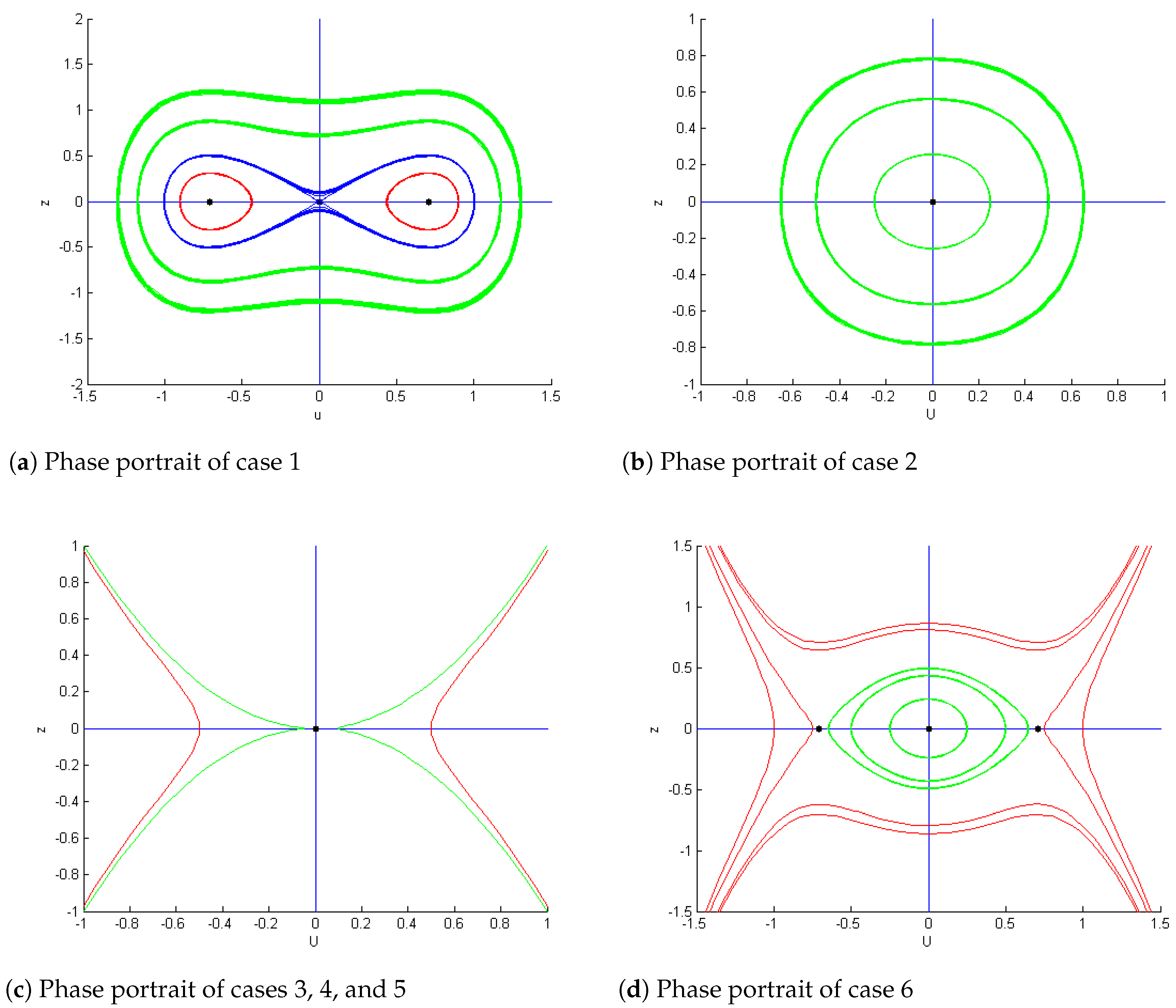
5. Bifurcation Behaviors and Phase Portrait

The bifurcation behavior of the given equation is analyzed in the next section. For this purpose, we employed the traveling wave transformation to transform Equation (1) to an ODE.

5.1. Planer Dynamical System

It is crucial to keep in mind that a dynamical system’s phase pictures might alter dramatically based on its equilibrium points. A solution for the associated NLPDE is shown by each orbit in the phase picture of a dynamical system. The bifurcation of Equation (16) is examined here. Due to the modification of the first equation, it is now an ensemble of first-order ODEs. For that, Equation (16) is used as shown below:

$${\mu }_1^2{\mathrm{Y}}^{″}-\left({\displaystyle \frac{p^2+r-{\lambda }_1{p}^3}{3\lambda p-1}}\right)\mathrm{Y}+2{\mathrm{Y}}^3=0.$$

(47)

The following is a demonstration of Equation (47):

$$\begin{array}{c}\hfill \left\{\begin{array}{c}{\displaystyle \frac{d{\mathrm{Y}}^{\prime }}{d\eta }}=z,\hfill \\ {\displaystyle \frac{dz}{d\eta }}=\left({\displaystyle \frac{p^2+r-{\lambda }_1{p}^3}{{\mu }^2\left(3{\lambda }_{1}p-1\right)}}\right)\mathrm{Y}-{\displaystyle \frac{2}{{\mu }_1^2}}{\mathrm{Y}}^3.\hfill \end{array}\right.\end{array}$$

(48)

5.2. Equilibrium Points

The roots of $\left({\displaystyle \frac{b^2+r-{\lambda }_1{b}^3}{{\mu }_1^2\left(3{\lambda }_{1}b-1\right)}}\right)\mathrm{Y}-{\displaystyle \frac{2}{{\mu }_1^2}}{\mathrm{Y}}^3$ are the equilibrium positions for perturbed system (48) on the axis $z=0$. Thus, we obtain

$${\displaystyle \frac{c_1}{c_2}}\mathrm{Y}-{\displaystyle \frac{2}{c_2}}{\mathrm{Y}}^3=0,$$

(49)

where

$$c_2={\mu }_1^2,c_1=\left({\displaystyle \frac{b^2+r-{\lambda }_1{b}^3}{{\mu }_1^2\left(3{\lambda }_{1}b-1\right)}}\right),$$

(50)

So, Equation (49) possesses a stable point ${\mathrm{Y}}_1=(0,0)$ if $c_1{c}_2<0$; however, the equilibrium points in dynamical system (48) are as follows if $c_1{c}_2>0$: ${\mathrm{Y}}_1=(0,0)$, ${\mathrm{Y}}_2=\left(\sqrt{{\displaystyle \frac{b}{2}}},0\right)$, ${\mathrm{Y}}_3=\left(\sqrt{-{\displaystyle \frac{b}{2}}},0\right)$. Consider that $M(\mathrm{Y},z)$ represents the linearized system’s coefficient matrix in dynamical system (48) at equilibrium point $\left(\mathrm{Y},z\right)$. It is called the Jacobian matrix of the system. According to a perturbed system, the determinant of the Jocobi matrix is as follows:

$$det\left[J(\mathrm{Y},z)\right]={\displaystyle \frac{6}{c_2}}\mathrm{Y}-{\displaystyle \frac{c_1}{c_2}}.$$

(51)

The stable point for system (48) is $(\mathrm{Y},0)$. According to the theory of planer dynamical systems, $(\mathrm{Y},0)$, the stable point of dynamical system (48) is a saddle when $det\left[J\right(\mathrm{Y},0\left)\right]<0$, a center when $det\left[J\right(\mathrm{Y},0\left)\right]>0$, or a cusp when $det\left[J\right(\mathrm{Y},0\left)\right]=0$.

The bifurcation of the planer dynamical system depends upon the parameters $c_2$ and $c_1$ in the perturbed system. Six cases are considered to be inside the parameters’ domain:

$$\begin{array}{cc}\hfill & R_1=\left[(c_2,c_1)\right|c_2>0,c_1>0],\hfill \\ \hfill & R_2=\left[(c_2,c_1)\right|c_2>0,c_1<0],\hfill \\ \hfill & R_3=\left[(c_2,c_1)\right|c_2>0,c_1=0],\hfill \\ \hfill & R_4=\left[(c_2,c_1)\right|c_2<0,c_1=0],\hfill \\ \hfill & R_5=\left[(c_2,c_1)\right|c_2<0,c_1<0],\hfill \\ \hfill & R_5=\left[(c_2,c_1)\right|c_2<0,c_1>0].\hfill \end{array}$$

With the use of Matlab and the previously indicated parameter, the phase picture of the dynamical system in plane $(\mathrm{Y},z)$ may be given.

• Case I:

The dynamical system (48) possesses three equilibrium values when $(c_2,c_1)\in R_1$, where the saddle is ${\mathrm{Y}}_1=(0,0)$. Moreover ${\mathrm{Y}}_{2,3}=\left(\pm \sqrt{{\displaystyle \frac{c_1}{2}}},0\right)$ are the two centers. Figure 1a represents the phase plots of this case for $c_2=1$ and $c_1=1$.

Figure 1. Qualitative analysis.

• Case II:

When $(c_2,c_1)\in R_2$, the system has one stable point, ${\mathrm{Y}}_1=(0,0)$, and it is a center. The phase plot for this case is shown in Figure 1b when $c_2=1$ and $c_1=-1$.

• Case III:

When $((c_2,c_1)\in R_3$, the system has one equilibrium, ${\mathrm{Y}}_1=(0,0)$, and it is a cusp. Figure 1c represents this case for $c_2=1,$ and $c_1=0$ using green lines.

• Case IV:

When $((c_2,c_1)\in R_4$, the system has one stable point, ${\mathrm{Y}}_1=(0,0)$, and, therefore, in this region ${\mathrm{Y}}_1$ is cusp. Figure 1c represents this case for $c_2=-1$ and $c_1=0$ using green lines.

• Case V:

Since the determinant of the Jacobi matrix (50) is negative, the system has one stable point, ${\mathrm{Y}}_1=(0,0)$, and it is saddle when $((c_2,c_1)\in R_5$. The phase plots for the current region is denoted by red lines in Figure 1c for $c_2=-1$ and $c_1=-1$.

• Case VI:

When $((c_2,c_1)\in R_6$, the system has three stable points where ${\mathrm{Y}}_1=(0,0)$ is the center point. Moreover, ${\mathrm{Y}}_{2,3}=\left(\pm \sqrt{{\displaystyle \frac{c_1}{2}}},0\right)$ are the two saddle points. Figure 1d represents the phase plots of this case for $c_2=-1$ and $c_1=1$.

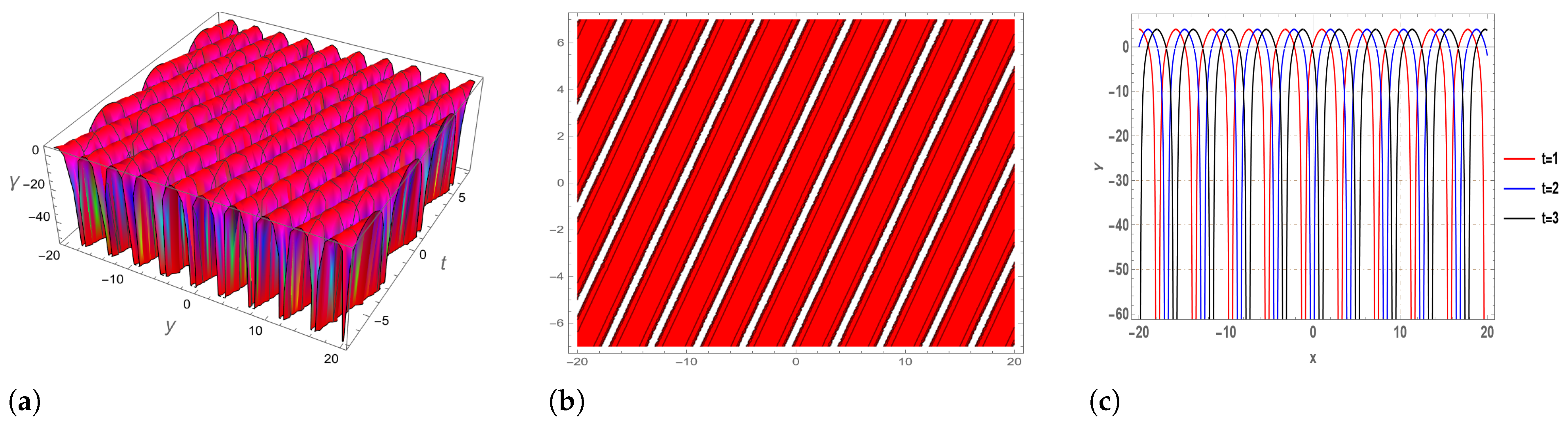
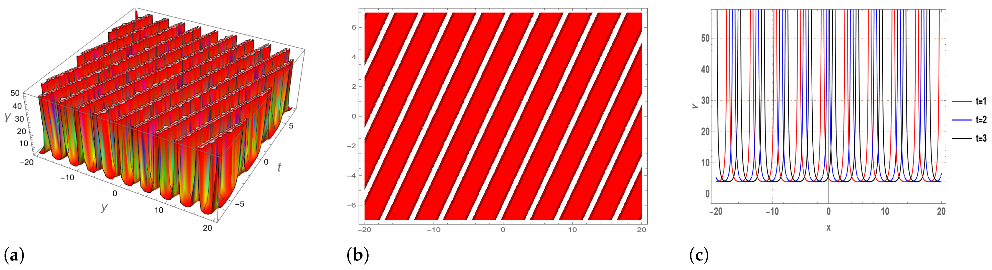
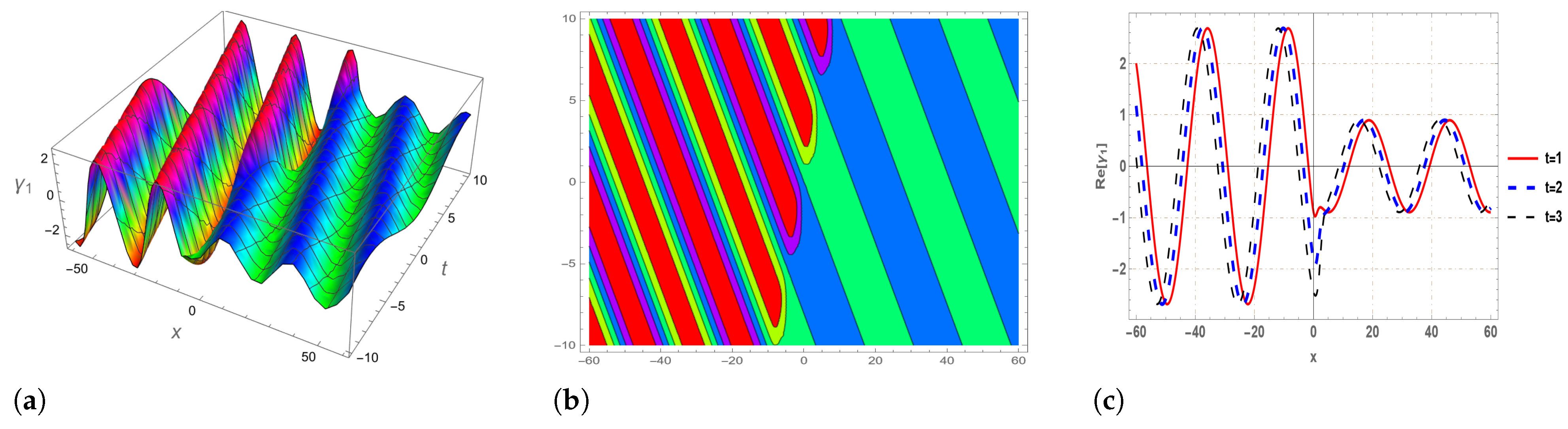
6. Graphical Representation

Examining the behavior of nonlinear wave phenomena through their graphical representations becomes more effective and advantageous when using exact solutions generated through mathematical computations. The exact solutions of the Hirota equation are graphically represented below:

Initially, we display $Re$[(26)] and $Abs$[(26)] in Figure 2 and Figure 3 and illustrate their 3D, contour, and 2D plots by setting parametric values such as $W_0=1.25$, $W_1=1.8$, $G_1=0.87$, ${\mu }_1=0.75$, $\zeta =1$, and $b=1.5$. The solution $Re$ [(26)] displays the periodic bright soliton in subplot (a), while subplots (b,c) depict its 2D and contour plots. The solution $Abs$ [(26)] displays the periodic dark solitary wave in subplot (a), while subplots (b,c) depict its 2D and contour plots. In Figure 4 and Figure 5, we represent 3D, contour, and 2D graphs by letting the parameters be $b=0.23$, ${\lambda }_1=1.06$, $r=0.39$, and $\zeta =0.78$ of the solutions obtained through the GBSOM. In Figure 4, subplot (a) shows a periodic bright solitary wave and subplots (b,c) depict the 2D and contour plots of $Re$ [(45)], respectively. The solution $Abs$ [(45)] displays the kink-type behavior in subplot (a) of Figure 5, while subplots (b,c) depict its associated 2D and contour plots.

Figure 2. The 3D (a), contour (b), and 2D (c) plots of $Re$ [Equation (26)].

Figure 3. The 3D (a), contour (b), and 2D (c) plots of $Abs$ [Equation (26)].

Figure 4. The 3D (a), contour (b), and 2D (c) plots of $Re$ [Equation (45)].

Figure 5. The 3D (a), contour (b), and 2D (c) plots of $Abs$ [Equation (45)].

7. Conclusions

In our research, we utilized the GERFM and GBSOM with a combination of traveling wave transformation generated from Lie point symmetry analysis to derive novel exact soliton solutions for the Hirota equation. This equation, with its distinctive components, offers a potentially more accurate representation of wave behavior in optical fibers and oceanic contexts compared to the conventional nonlinear Schrödinger equation. The exact solutions obtained from these approaches include traveling wave solutions, yielding singular, periodic, and kink solitons. Although the GERFM and GBSOM were successful in analytically solving the Hirota equation, some limitations remain as they do not yield bright solitons. Furthermore, we performed a bifurcation analysis to explore the dynamic behavior of the planar system under varied parameters, with each scenario represented by phase portraits. Our results reveal unique solutions that were previously unreported, and the methodologies presented can extend to other complex nonlinear systems.

References

- Mollenauer, L.F.; Gordon, J.P. Solitons in Optical Fibers: Fundamentals and Applications; Elsevier: Amsterdam, The Netherlands, 2006. [Google Scholar]
- Kumar, S.; Ma, W.X.; Dhiman, S.K.; Chauhan, A. Lie group analysis with the optimal system, generalized invariant solutions, and an enormous variety of different wave profiles for the higher-dimensional modified dispersive water wave system of equations. Eur. Phys. J. Plus 2023, 138, 434. [Google Scholar] [CrossRef]
- Butt, A.R.; Raza, N.; Inc, M.; Alqahtani, R.T. Complexitons, Bilinear forms and Bilinear Bäcklund transformation of a (2 + 1)-dimensional Boiti–Leon–Manna–Pempinelli model describing incompressible fluid. Chaos Solitons Fractals 2023, 168, 113201. [Google Scholar] [CrossRef]
- Hong, B. Assorted exact explicit solutions for the generalized Atangana’s fractional BBM–Burgers equation with the dissipative term. Front. Phys. 2022, 10, 1071200. [Google Scholar] [CrossRef]
- Arnous, A.H.; Seadawy, A.R.; Alqahtani, R.T.; Biswas, A. Optical solitons with complex Ginzburg–Landau equation by modified simple equation method. Optik 2017, 144, 475–480. [Google Scholar] [CrossRef]
- Jawad, A.J.; Petković, M.D.; Biswas, A. Modified simple equation method for nonlinear evolution equations. Appl. Math. Comput. 2010, 217, 869–877. [Google Scholar]
- Kuo, R.J.; Setiawan, M.R.; Nguyen, T.P. Sequential clustering and classification using deep learning technique and multi-objective sine-cosine algorithm. Comput. Ind. Eng. 2022, 173, 108695. [Google Scholar] [CrossRef]
- Albalawi, W.; Raza, N.; Arshed, S.; Farman, M.; Nisar, K.S.; Abdel-Aty, A.H. Chaotic behavior and construction of a variety of wave structures related to a new form of generalized q-Deformed sinh-Gordon model using couple of integration norms. AIMS Math. 2024, 9, 9536–9555. [Google Scholar] [CrossRef]
- Sulaiman, T.A.; Yusuf, A.; Atangana, A. New lump, lump-kink, breather waves and other interaction solutions to the (3+ 1)-dimensional soliton equation. Commun. Theor. Phys. 2020, 72, 085004. [Google Scholar] [CrossRef]
- Yusuf, A.; Sulaiman, T.A.; Inc, M.; Bayram, M. Breather wave, lump-periodic solutions and some other interaction phenomena to the Caudrey–Dodd–Gibbon equation. Eur. Phys. J. Plus 2020, 135, 1–8. [Google Scholar] [CrossRef]
- Murad, M.A.; Iqbal, M.; Arnous, A.H.; Biswas, A.; Yildirim, Y.; Alshomrani, A.S. Optical dromions with fractional temporal evolution by enhanced modified tanh expansion approach. J. Opt. 2024, 1–10. [Google Scholar] [CrossRef]
- Sivasundaram, S.; Kumar, A.; Singh, R.K. On the complex properties to the first equation of the KadomtsevPetviashvili hierarchy. Int. J. Math. Comput. Eng. 2024, 2, 71–84. [Google Scholar] [CrossRef]
- Raza, N.; Jhangeer, A.; Arshad, S.; Butt, A.R.; Chu, Y. Dynamical analysis and phase portraits of two-mode waves in different media. Chaos 2020, 19, 103650. [Google Scholar] [CrossRef]
- Saha, A. Bifurcation, periodic and chaotic motions of the modified equal width-Burgers (MEW-Burgers) equation with external periodic perturbation. Nonlinear Dyn. 2017, 87, 2193–2201. [Google Scholar] [CrossRef]
- Elmandouha, A.A.; Ibrahim, A.G. Bifurcation and travelling wave solutions for a (2+1)-dimensional KdV equation. J. King Saud Univ.-Sci. 2020, 14, 139–147. [Google Scholar] [CrossRef]
- Salam, M.A.; Mondal, M.; Ali, M.S.; Dey, P. The analysis of exact solitons solutions in monomode optical fibers to the generalized nonlinear Schrödinger system by the compatible techniques. Int. J. Math. Comput. Eng. 2023, 1, 149–170. [Google Scholar]
- Hirota, R. Exact envelope-soliton solutions of a nonlinear wave equation. J. Math. Phys. 1973, 14, 805–809. [Google Scholar] [CrossRef]
- Hirota, R. The Direct Method in Soliton Theory; Cambridge University Press: Cambridge, UK, 1987. [Google Scholar]
- Bulut, H.; Sulaiman, T.A.; Baskonus, H.M.; Akturk, T. On the bright and singular optical solitons to the (2+1)- dimensional NLS and the Hirota models. Opt. Quant. Electron. 2018, 50, 134. [Google Scholar] [CrossRef]
- Eslami, M.; Mirzazadeh, M.A.; Neirameh, A. New exact wave solutions for Hirota model. Pramana-J. Phys. 2015, 84, 3–8. [Google Scholar] [CrossRef]
- Shu, J.J. Exact n-envelope-soliton solutions of the Hirota model. Opt. Appl. 2003, 33, 539–546. [Google Scholar]
- Li, L.; Wu, Z.; Wang, L.; He, J. High-order rogue waves for the Hirota equation. Ann. Phys. 2013, 334, 198–211. [Google Scholar] [CrossRef]
- Wang, P.; Tian, B.; Liu, W.J.; Li, M.; Sun, K. Soliton solutions for a generalized inhomogeneous variable-coefficient Hirota model with symbolic computation. Stud. Appl. Math. 2010, 125, 213–222. [Google Scholar]
- Demontisa, F.; Ortenzib, G.; van der Mee, C. Exact solutions of the Hirota model and vortex filaments motion. Phys. D 2015, 313, 61–80. [Google Scholar] [CrossRef]
- Dhiman, S.K.; Kumar, S. Analyzing specific waves and various dynamics of multi-peakons in (3 + 1)-dimensional p-type equation using a newly created methodology. Nonlinear Dyn. 2024, 112, 10277–10290. [Google Scholar] [CrossRef]
- Yang, X.F.; Deng, Z.C.; Wei, Y. A Riccati-Bernoulli sub-ODE method for nonlinear partial differential equations and its application. Adv. Differ. Equ. 2015, 117. [Google Scholar] [CrossRef]
- Salam, M.A.; Mondal, M.; Ali, M.S.; Dey, P. Traveling Wave Solutions of Regularized Long-Wave Equation. J. Comput. Math. Sci. 2015, 6, 171–178. [Google Scholar]
Disclaimer/Publisher’s Note: The statements, opinions and data contained in all publications are solely those of the individual author(s) and contributor(s) and not of MDPI and/or the editor(s). MDPI and/or the editor(s) disclaim responsibility for any injury to people or property resulting from any ideas, methods, instructions or products referred to in the content. |
© 2024 by the authors. Licensee MDPI, Basel, Switzerland. This article is an open access article distributed under the terms and conditions of the Creative Commons Attribution (CC BY) license (https://creativecommons.org/licenses/by/4.0/).