The Riemann–Hilbert Approach to the Higher-Order Gerdjikov–Ivanov Equation on the Half Line

Abstract

The Fokas method exhibits remarkable versatility in solving boundary value problems associated with both linear and nonlinear partial differential equations, particularly when conventional approaches encounter challenges in handling intricate boundary conditions. The existing literature often lacks the incorporation of unconventional boundary conditions, and this study addresses this issue by extending the application of the Fokas method to the higher-order Gerdjikov-Ivanov equation on the half line $(-\infty ,0]$. We have demonstrated the exclusive representation of the potential function $u(z,t)$ in the higher-order Gerdjikov–Ivanov equation through the solution of a Riemann–Hilbert problem. The characteristic function is partitioned on the complex plane, and we obtain the jump matrix between each partition based on the positive and negative values of the partition as well as the spectral matrix determined by the initial data and boundary value data. The findings suggest that the spectral functions are not mutually independent; instead, they conform to a global relationship. The novel aspect of this study is the application of the Fokas method to a previously unexplored case, contributing to the theoretical and practical understanding of complex partial differential equations and filling a gap in the treatment of boundary conditions.

1. Introduction

It is well known that the initial value problems of many classical integrable systems can be solved by the inverse scattering method [1]. However, the inverse scattering method is not suitable for every nonlinear Equation [2,3]. The determination of the solution to the nonlinear equation is influenced by both the initial boundary value and is not solely reliant on the initial value. This indicates that the inverse scattering method cannot be applied in this scenario, necessitating the exploration of alternative approaches for analyzing the initial boundary value problem. In 1997, Fokas [4,5,6] introduced the Fokas method, a special inverse scattering method that effectively solves the initial boundary value problem of integrable equations by utilizing the concept of the inverse scattering method on a line. The Fokas method also expresses the solution of the initial boundary value problem as the corresponding solution of the Riemann–Hilbert problem. However, when analyzing the initial boundary value problem in the complex plane, we encounter the challenge of interdependent boundary values, where any change in a single value affects the entire solution. Consequently, constructing a relevant Riemann–Hilbert problem necessitates considering multiple scenarios of initial boundary values and selecting the appropriate one. Lenells [7,8,9,10,11] extended this method for the first time and studied the initial boundary value problem of the Degasperis-Procesi equation on the half line [12]. After this, Its [13,14], Monvel [15,16,17], Lenells [7,8,9,10,11,12], Fan and Xu [18,19,20,21,22], and Zhang and Hu [23,24,25,26,27,28,29,30,31] et al. began to pay attention to the initial boundary value problem of integrable systems and extended the Fokas method.

Equation (1), commonly known as the GI equation, was initially identified by Gerdjikov and Ivanov in their work [32]. The inverse scattering method can be used to solve the GI equation. The significance of this equation lies in its integrability, which makes it valuable for both mathematical analysis and physical applications. The propagation of light pulses in optical fibers is effectively described by the GI equation [33,34,35,36], which plays a crucial role. Nonlinear effects occurring in optical fibers can result in self-phase modulation and group-velocity dispersion of optical pulses. Consequently, the GI equation aids in designing and optimizing communication systems that utilize optical fiber technology. Additionally, the GI equation finds applications in studying how shallow water waves propagate and interact. By solving this equation, one can analyze the behavior of nonlinear water waves regarding stability and rupture, thereby making significant contributions to fields such as ocean engineering and environmental science.

$$i{u}_t+u_{zz}-i{u}^2{u}_z^{*}+{\displaystyle \frac{1}{2}}{\left|u\right|}^{4}u=0.$$

(1)

When considering certain nonlinear effects of a higher order, Equation (1) can be seen as an extension of NLS, also known as DNLS III. Equation (2), referred to as the DNLS I equation, is known as the Kaup–Newell Equation [37]. It is a dispersion equation commonly used in magnetohydrodynamics studies.

$$i{u}_t+u_{zz}+i{\left(u^2{u}^{*}\right)}_z=0.$$

(2)

Equation (3), referred to as the C-L-L Equation [38], is known as the Chen–Lee–Liu (C-L-L) equation in optical models for ultra-short pulses.

$$i{u}_t+u_{zz}+iu{u}^{*}{u}_z=0.$$

(3)

The main emphasis of our paper is directed towards the higher-order Gerdjikov–Ivanov Equation [39,40].

$$u_t+{\displaystyle \frac{1}{2}}{u}_{zzz}-{\displaystyle \frac{3}{2}}iu{u}_z{u}_z^{*}+{\displaystyle \frac{3}{4}}{\left|u\right|}^4{u}_z=0.$$

(4)

In recent years, extensive studies have been conducted regarding the GI equation, such as its Darboux transformation and hamilton structure, algebraic geometry solution, transdynamic wave solution, and the determination of the asymptotic behavior for the solution to the GI equation. For the higher order Gerdjikov–Ivanov equation, Guo [41] has successfully constructed rogue wave solutions using determinants, while Liu [42] has investigated non-local higher order Gerdjikov–Ivanov equation and discovered that the solutions of these equations depend not only on temporal and spatial variables but also on non-local variables. However, the Fokas method has not been utilized to investigate the higher order Gerdjikov–Ivanov equation. The aim of this study is to examine the initial boundary value problem associated with the Gerdjikov–Ivanov equation of higher order on the half line. Figure 1 shows the area we want to analyze.

Figure 1. The $(z,t)$-domain.

Sides $\{-\infty <z\le 0,t=L\}$, $\{z=0,0\le t\le T\}$ and $\{-\infty <z\le 0,t=0\}$ are called sides $\left(1\right),\left(2\right),\left(3\right)$, respectively, as shown in Figure 1.

Assuming that solution $u(z,t)$ to higher-order Gerdjikov–Ivanov equation exists, we define the initial value

$$u_0\left(z\right)=u(z,0),-\infty <z<0,$$

(5)

the boundary value

$$f_0\left(t\right)=u(0,t), f_1\left(t\right)=u_z(0,t), f_2\left(t\right)=u_{zz}(0,t), 0<t<T.$$

(6)

The solution of the equation can be represented using the resolution of the matrix Riemann–Hilbert problem.

The higher-order Gerdjikov–Ivanov equation finds extensive applications in the domains of plasma physics and nonlinear optics. In plasma physics [43,44,45,46], the equation can indicate the direction and angle of propagation for both small-amplitude nonlinear Alfvén waves and large-amplitude nonlinear Alfvén waves. The higher-order Gerdjikov–Ivanov equation has the potential to characterize a weak bound state of solitons, and could be relevant in investigating the propagation behavior of solitons that have similar velocities and amplitudes. In nonlinear optics [33,34,35,36], the utilization of femtosecond optical pulses has attracted considerable attention due to its extensive implementation in communication and routing systems for flow control. To accurately model this phenomenon, the higher-order Gerdjikov–Ivanov equation is necessary. Specifically, in the context of optical fibers, the higher-order Gerdjikov–Ivanov equation serves as a suitable model for long-distance high-bit-rate transmission systems involving the propagation of optical solitons in single-mode fibers.

In this study, we employ the Fokas method to analyze the initial boundary value of the finite interval $(-\infty ,0]$. The arrangement of this article is outlined below. In Section 2, we give the conclusions related to the higher-order Gerdjikov–Ivanov equation, and partition the characteristic function to discuss the relationship between each partition. In Section 3, jump matrix has an explicit dependence, and the spectral functions $\left\{\chi \right(\beta ),k(\beta \left)\right\}$ and $\left\{X\right(\beta ),K(\beta \left)\right\}$ are decided by the initial condition $u_0\left(z\right)=u(z,0)$ and boundary values condition $f_0\left(t\right)=u(0,t)$, $f_1\left(t\right)=u_z(0,t)$ and $f_2\left(t\right)=u_{zz}(0,t)$, respectively. Spectral functions demonstrate interdependence; they have a global relationship and can be connected by a consistent condition. In Section 4, this paper is summarized and the future work is planned.

2. Basic Riemann–Hilbert Problem

2.1. Formulas and Symbols

• ${\theta }_3=\left(\begin{array}{cc}1& 0\\ 0& -1\end{array}\right)$ denotes the Pauli’s matrix [47];
• Two $2\times 2$ matrices, $X,K$, have the matrix commutator $[X,K]=XK-KX$;
• The matrix commutator with ${\theta }_3$, ${\widehat{\theta }}_{3}X=[{\theta }_3,X]$ is shown by ${\widehat{\theta }}_3$. After that, $e^{{\widehat{\theta }}_3}$ is simple to calculate: $e^{{\widehat{\theta }}_3}X=e^{{\theta }_3}X{e}^{-{\theta }_3}$;
• The complex conjugate of $h(•)$ is denoted by $\overline{h(•)}$ if $h(•)$ is a function.

2.2. Lax Pair

Recursive operators, GI hierarchies, and Lax pairs for higher-order GI equations can be obtained in Zhu [40]. In Fan’s paper [48], it is proven that the equation is Liouville-integrable and has multiple Hamiltonian structures. The Lax pair is satisfied by the higher-order Gerdjikov–Ivanov equation for any $\beta \in \mathbb{C}$:

$${\partial }_z\mathsf{\Psi }(z,t;\beta )=M(z,t;\beta )\mathsf{\Psi }(z,t;\beta ),{\partial }_t\mathsf{\Psi }(z,t;\beta )=N(z,t;\beta )\mathsf{\Psi }(z,t;\beta ),$$

(7)

where

$$\begin{array}{c}M(z,t;\beta )=-i{\beta }^2{\theta }_3+\beta R-{\displaystyle \frac{i}{2}}{R}^2{\theta }_3,\hfill \\ N(z,t;\beta )=-2i{\beta }^6{\theta }_3+2{\beta }^{5}R-i{\beta }^4{R}^2{\theta }_3+i{\beta }^3{\theta }_3{R}_z+T_2{\beta }^2+T_1\beta +T_0,\hfill \\ T_0={\displaystyle \frac{i}{4}}(R{R}_{zz}+R_{zz}R){\theta }_3-{\displaystyle \frac{i}{4}}{R}_z^2{\theta }_3+{\displaystyle \frac{i}{8}}{R}^6{\theta }_3,\hfill \\ T_1=-{\displaystyle \frac{1}{2}}{R}_{zz}+{\displaystyle \frac{i}{2}}R{R}_{z}R{\theta }_3-{\displaystyle \frac{1}{4}}{R}^5,\hfill \\ T_2=-{\displaystyle \frac{1}{2}}(R{R}_z-R_{z}R)+{\displaystyle \frac{i}{4}}{R}^4{\theta }_3.\hfill \end{array}$$

(8)

The equation’s initial condition is given by $u_0\left(z\right)=u(z,0)$, while its boundary conditions are represented as $f_0\left(t\right)=u(0,t)$, $f_1\left(t\right)=u_z(0,t)$, and $f_2\left(t\right)=u_{zz}(0,t)$. Assuming

$$\psi =\mathsf{\Psi }{e}^{-i({\beta }^{2}z+2{\beta }^{6}t){\theta }_3},-\infty <z\le 0,0\le t\le T,$$

(9)

we acquire the Lax pair that has equal value

$$\begin{array}{c}{\mathsf{\Psi }}_z+i{\beta }^2[{\theta }_3,\mathsf{\Psi }]=(\beta R-{\displaystyle \frac{i}{2}}{R}^2{\theta }_3)\mathsf{\Psi },\hfill \\ {\mathsf{\Psi }}_t+2i{\beta }^6[{\theta }_3,\mathsf{\Psi }]=(2{\beta }^{5}R-i{\beta }^4{R}^2{\theta }_3+i{\beta }^3{\theta }_3{R}_x+T_2{\beta }^2+T_1\beta +T_0)\mathsf{\Psi },\hfill \end{array}$$

(10)

where

$$R=u{\theta }_{+}+v{\theta }_{-},{\theta }_{+}=\left(\begin{array}{cc}0& 1\\ 0& 0\end{array}\right),{\theta }_{-}=\left(\begin{array}{cc}0& 0\\ 1& 0\end{array}\right).$$

(11)

The Lax pair can be formulated as total differentials

$$d\left(e^{i({\beta }^{2}z+2{\beta }^{6}t){\widehat{\theta }}_3}\psi (z,t;\beta )\right)=e^{i({\beta }^{2}z+2{\beta }^{6}t){\widehat{\theta }}_3}U(z,t;\beta )\psi ,-\infty <z\le 0,0\le t\le T,$$

(12)

where

$$\begin{array}{c}U(z,t;\beta )=U_1(z,t;\beta )dz+U_2(z,t;\beta )dt,\hfill \\ U_1(z,t;\beta )=\beta R-{\displaystyle \frac{i}{2}}{R}^2{\theta }_3,U_2(z,t;\beta )=2{\beta }^{5}R-i{\beta }^4{R}^2{\theta }_3+i{\beta }^3{\theta }_3{R}_z+{\beta }^2{T}_2+\beta T_1+T_0.\hfill \end{array}$$

To address the inverse spectral problem through the Riemann–Hilbert approach, our objective is to find a solution to the spectral problem that converges towards an identity matrix as $\beta \to \infty$. We will use the Lenells method [7,8,9,10,11,12] to transform (12) into the expected asymptotic behavior since the result does not meet this property.

Suppose that a solution to (12) has the following form:

$$\psi (z,t;\beta )=G_0+{\displaystyle \frac{G_1}{\beta }}+{\displaystyle \frac{G_2}{{\beta }^2}}+{\displaystyle \frac{G_3}{{\beta }^3}}+{\displaystyle \frac{G_4}{{\beta }^4}}+{\displaystyle \frac{G_5}{{\beta }^5}}+\mathcal{O}\left({\displaystyle \frac{1}{{\beta }^6}}\right),\beta \to \infty ,$$

where $G_0,G_1,G_2,G_3,G_4,G_5$ are independent of $\beta$. After matching the identical order of $\beta$ and replacing the aforementioned expansion applied to the first equation of (10), we obtain

$$\begin{array}{c}O\left({\beta }^2\right):i[{\theta }_3,G_0]=0,\hfill \\ O\left(\beta \right):i[{\theta }_3,G_1]=R{G}_0,\hfill \\ O\left(1\right):G_{0x}+i[{\theta }_3,G_2]=R{G}_1-{\displaystyle \frac{i}{2}}{R}^2{\theta }_3{G}_0.\hfill \end{array}$$

$G_0$ is represented by a matrix with diagonal elements, and let $G_0=\left(\begin{array}{cc}{G}_0^{11}& 0\\ 0& G_0^{22}\end{array}\right)$. Based on $O\left(\beta \right)$, we have

$$G_1^{\left(o\right)}=\left(\begin{array}{cc}0& -{\displaystyle \frac{i}{2}}u{G}_0^{22}\\ {\displaystyle \frac{i}{2}}v{G}_0^{11}& 0\end{array}\right),$$

where the off-diagonal part of $G_1$ is denoted as $G_1^{\left(o\right)}$. From $O\left(1\right)$, we have

$$G_{0z}=-iuv{\theta }_3{G}_0.$$

(13)

Bringing the asymptotic expansion into (10), we obtain

$$\begin{array}{c}O\left({\beta }^6\right):2i[{\theta }_3,G_0]=0,\hfill \\ O\left({\beta }^5\right):2i[{\theta }_3,G_1]=2R{G}_0,\hfill \\ O\left({\beta }^4\right):2i[{\theta }_3,G_2]=2R{G}_1-i{R}^2{\theta }_3{G}_0,\hfill \\ O\left({\beta }^3\right):2i[{\theta }_3,G_3]=2R{G}_2-i{R}^2{G}_1{\theta }_3+i{\theta }_3{R}_x{G}_0,\hfill \\ O\left({\beta }^2\right):2i[{\theta }_3,G_4]=2R{G}_3-i{R}^2{G}_2{\theta }_3+i{\theta }_3{R}_x{G}_1+T_2{G}_0,\hfill \\ O\left(\beta \right):2i[{\theta }_3,G_5]=2R{G}_4-i{R}^2{G}_3{\theta }_3+i{\theta }_3{R}_x{G}_2+T_2{G}_1+T_1{G}_0,\hfill \\ O\left(1\right):G_{0t}=2R{G}_5-i{R}^2{G}_4{\theta }_3+i{\theta }_3{R}_x{G}_3+T_2{G}_2+T_1{G}_1+T_0{G}_0.\hfill \end{array}$$

After calculation, it is deduced by the form $O\left(1\right)$

$$G_{0t}=({\displaystyle \frac{i}{2}}{u}_{zz}v+{\displaystyle \frac{i}{2}}u{v}_{zz}-{\displaystyle \frac{i}{2}}{u}_z{v}_z+{\displaystyle \frac{i}{4}}{u}^3{v}^3){\theta }_3{G}_0.$$

(14)

Equation (4) has the conservation law

$${\left(uv\right)}_t={(-{\displaystyle \frac{1}{2}}{u}_{zz}v-{\displaystyle \frac{1}{2}}u{v}_{zz}+{\displaystyle \frac{1}{2}}{u}_z{v}_z-{\displaystyle \frac{1}{4}}{u}^3{v}^3)}_z.$$

(15)

Equations (13) and (14) for $G_0$ are consistent; we are able to define it as follows:

$$G_0(z,t)=exp(i{\int }_{(z_0,t_0)}^{(z,t)}\Delta {\theta }_3),$$

(16)

where $\Delta (z,t)={\Delta }_1(z,t)dz+{\Delta }_2(z,t)dt$, ${\Delta }_1(z,t)=-uv$, ${\Delta }_2(z,t)={\displaystyle \frac{1}{2}}{u}_{zz}v+{\displaystyle \frac{1}{2}}u{v}_{zz}-{\displaystyle \frac{1}{2}}{u}_z{v}_z-{\displaystyle \frac{1}{4}}{u}^3{v}^3$, $(z_0,t_0)\in G$, simultaneity, we indicate $(z_0,t_0)=(0,0)$ to make computations easier.

Since the integral in (16) is path-independent, the following new function $E(z,t;\beta )$ is introduced

$$\psi (z,t;\beta )=e^{i{\int }_{(0,0)}^{(z,t)}\Delta {\widehat{\theta }}_3}E(z,t;\beta )D_0(x,t),-\infty <z\le 0,0\le t\le T.$$

(17)

The Lax pair of (12) is identical by simple computation

$$d\left(e^{i({\beta }^{2}z+2{\beta }^{6}t){\widehat{\theta }}_3}E(z,t;\beta )\right)=A(z,t;\beta ),\beta \in \mathbb{C},$$

(18)

where

$$\begin{array}{c}A(z,t;\beta )=e^{i({\beta }^{2}z+2{\beta }^{6}t){\widehat{\theta }}_3}B(z,t;\beta )E(z,t;\beta ),\hfill \\ B(z,t;\beta )=B_1(z,t;\beta )dx+B_2(z,t;\beta )dt=e^{-i{\int }_{(0,0)}^{(z,t)}\Delta {\widehat{\theta }}_3}(U(z,t;\beta )-i\Delta {\theta }_3).\hfill \end{array}$$

The formulas above can be modified by substituting the definitions of $U(z,t;\beta )$ and $\Delta$ to obtain $B_1$ and $B_2.$

$$\begin{array}{c}{B}_1(z,t;\beta )=\left(\begin{array}{cc}{\displaystyle \frac{i}{2}}uv& \beta u{e}^{-2i{\int }_{(0,0)}^{(z,t)}\Delta }\\ \beta vs.e^{2i{\int }_{(0,0)}^{(z,t)}\Delta }& -{\displaystyle \frac{i}{2}}uv\end{array}\right),\hfill \\ B_2(z,t;\beta )=\left(\begin{array}{cc}{B}_2^{11}& B_2^{12}\\ B_2^{21}& B_2^{22}\end{array}\right).\hfill \\ B_2^{11}=-i{\beta }^{4}uv-{\displaystyle \frac{1}{2}}{\beta }^2(u{v}_z-u_{z}v)+{\displaystyle \frac{i}{4}}{\beta }^2{u}^2{v}^2-{\displaystyle \frac{i}{4}}{u}_{zz}v-{\displaystyle \frac{i}{4}}u{v}_{zz}+{\displaystyle \frac{i}{4}}{u}_z{v}_z+{\displaystyle \frac{3}{8}}i{u}^3{v}^3,\hfill \\ B_2^{12}=(2{\beta }^{5}u+i{\beta }^3{u}_z-{\displaystyle \frac{1}{2}}\beta u_{zz}-{\displaystyle \frac{i}{2}}\beta u^2{v}_z-{\displaystyle \frac{1}{4}}\beta u^3{v}^2)e^{-2i{\int }_{(0,0)}^{(z,t)}\Delta },\hfill \\ B_2^{21}=(2{\beta }^{5}v-i{\beta }^3{v}_z-{\displaystyle \frac{1}{2}}\beta v_{zz}+{\displaystyle \frac{i}{2}}\beta u_z{v}^2-{\displaystyle \frac{1}{4}}\beta u^2{v}^3)e^{2i{\int }_{(0,0)}^{(z,t)}\Delta },\hfill \\ B_2^{22}=i{\beta }^{4}uv-{\displaystyle \frac{1}{2}}{\beta }^2(u_{z}v-u{v}_z)-{\displaystyle \frac{i}{4}}{\beta }^2{u}^2{v}^2+{\displaystyle \frac{i}{4}}{u}_{zz}v+{\displaystyle \frac{i}{4}}u{v}_{zz}-{\displaystyle \frac{i}{4}}{u}_z{v}_z-{\displaystyle \frac{3}{8}}i{u}^3{v}^3.\hfill \end{array}$$

Then, the expression for $E(z,t;\beta )$ in Equation (18) can be derived

$$\begin{array}{c}{E}_x+i{\beta }^2[{\theta }_3,E]=B_{1}E,\hfill \\ E_y+2i{\beta }^6[{\theta }_3,E]=B_{2}E,\hfill \end{array}$$

(19)

where $-\infty <z\le 0,0\le t\le T,\beta \in \mathbb{C}.$

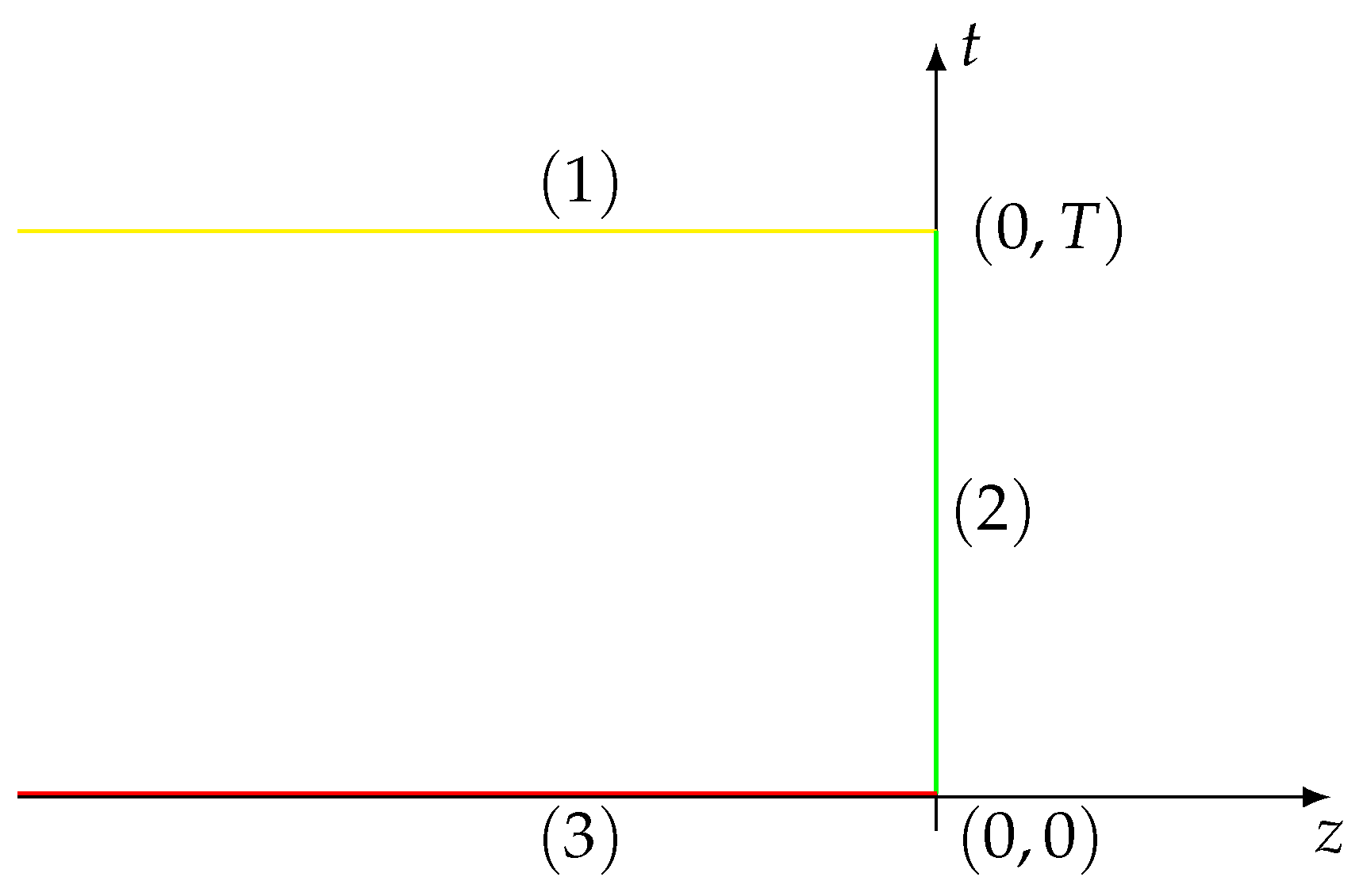
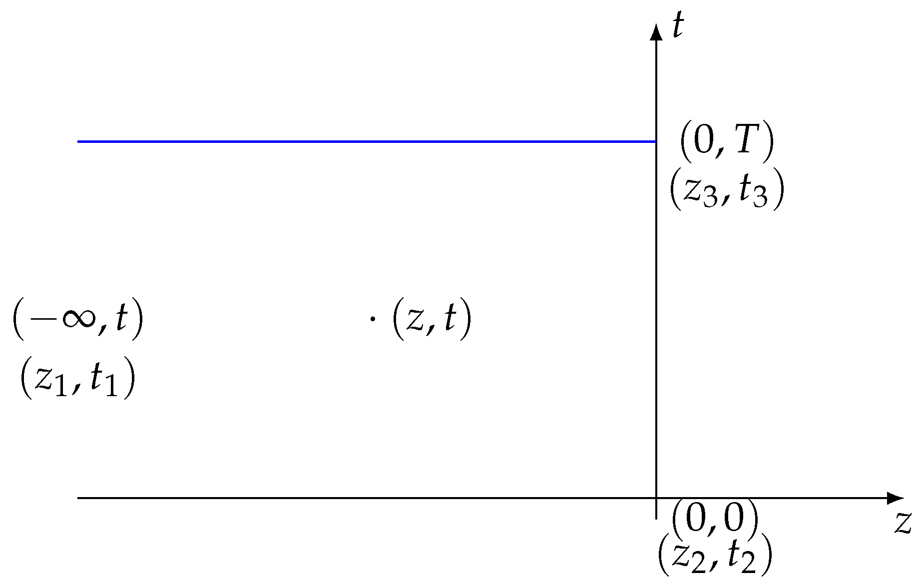
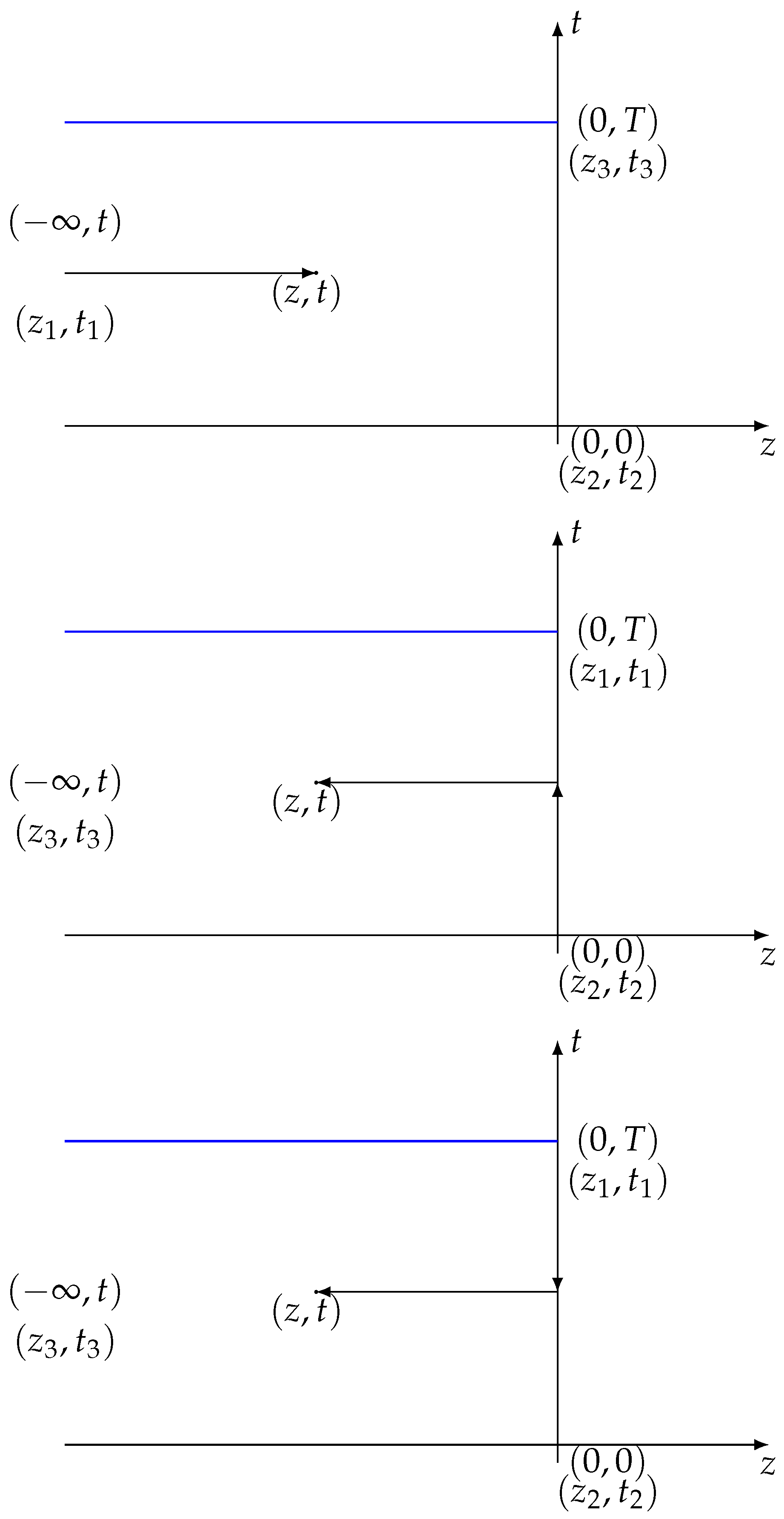
2.3. Three Eigenfunctions

We hypothesize the existence of $u(z,t)$ and a sufficient smoothness of $G=\{-\infty <z\le 0,0\le t\le T\}$. From Equation (18), three eigenfunctions $E_k(z,t,\beta )(k=1,2,3.)$ are provided as

$$E_k(z,t;\beta )=I+{\int }_{(z_k,t_k)}^{(z,t)}{e}^{-i({\beta }^{2}z+2{\beta }^{6}t){\widehat{\theta }}_3}A(\xi ,\tau ,\beta ),-\infty <z<0,0<t<T.$$

(20)

The integral represents a continuous curve from $(z_k,t_k)$ to $(z,t)$, where $(z_1,t_1)=(-\infty ,t),$$(z_2,t_2)=(0,0),(z_3,t_3)=(0,T)$. Please refer to Figure 2.

Figure 2. The three points in the $(z,t)$-domain.

Some domain in the complex $\beta$-plane defines the functions $E_1$, $E_2$, and $E_3$. We choose a unique integral path that is parallel to the coordinate axis, as indicated in Figure 3, since the calculation of Equation (16) is not influenced by the specific path chosen.

Figure 3. $l_1,l_2,l_3$ in the $(z,t)$-domain.

These paths imply the inequality that follows

$$\begin{array}{c}(z_1,t_1)\to (z,t):-\infty <\xi <z,\hfill \\ (z_2,t_2)\to (z,t):z<\xi <0,0<\tau <t,\hfill \\ (z_3,t_3)\to (z,t):z<\xi <0,t<\tau <T.\hfill \end{array}$$

Based on the above analysis, we have obtained

$$\begin{array}{c}\begin{array}{c}\hfill E_1(z,t;\beta )=I+{\int }_{-\infty }^z{e}^{i{\beta }^2(\xi -z){\widehat{\theta }}_3}\left(B_1{\mu }_1\right)(\xi ,t,\beta )d\xi ,\\ \hfill E_2(z,t;\beta )=I-{\int }_z^0{e}^{i{\beta }^2(\xi -z){\widehat{\theta }}_3}\left(B_1{\mu }_2\right)(\xi ,t,\beta )d\xi \\ \hfill +e^{-i{\beta }^{2}z{\widehat{\theta }}_3}{\int }_0^t{e}^{2i{\beta }^4(\tau -t){\widehat{\theta }}_3}\left(B_2{\mu }_2\right)(0,\tau ,\beta )d\tau ,\\ \hfill E_3(z,t;\beta )=I-{\int }_z^0{e}^{i{\beta }^2(\xi -z){\widehat{\theta }}_3}\left(B_1{\mu }_3\right)(\xi ,t,\beta )d\xi \\ \hfill -e^{-i{\beta }^{2}z{\widehat{\theta }}_3}{\int }_t^T{e}^{2i{\beta }^4(\tau -t){\widehat{\theta }}_3}\left(B_2{\mu }_3\right)(0,\tau ,\beta )d\tau .\end{array}\hfill \end{array}$$

(21)

Let us assume that $E_k(z,t;\beta )=I+\mathcal{O}\left({\displaystyle \frac{1}{\beta }}\right)$ (for $k=1,2,3$) as $\beta \to \infty$, given the dependence of $B_1(z,t;\beta )$ and $B_2(z,t;\beta )$ on $\beta$. Using the inequality above, we determine that they are bounded, allowing us to divide the complex $\beta$-plane into the following 12 regions

$$\begin{array}{c}{E}_1^{\left(1\right)}(z,t;\beta ):(z_1,t_1)\to (z,t):\{\mathrm{Im}{\beta }^2\ge 0\},\hfill \\ E_2^{\left(1\right)}(z,t;\beta ):(z_2,t_2)\to (z,t):\{\mathrm{Im}{\beta }^2\le 0\}\bigcap \{\mathrm{Im}{\beta }^6\ge 0\},\hfill \\ E_3^{\left(1\right)}(z,t;\beta ):(z_3,t_3)\to (z,t):\{\mathrm{Im}{\beta }^2\le 0\}\bigcap \{\mathrm{Im}{\beta }^6\le 0\}.\hfill \end{array}$$

The second column is the inverse of the first column in Equation (20), so the result of the second column is opposite to that of the first column, which is bounded in

$$\begin{array}{c}{E}_1^{\left(2\right)}(z,t;\beta ):(z_1,t_1)\to (z,t):\{\mathrm{Im}{\beta }^2\le 0\},\hfill \\ E_2^{\left(2\right)}(z,t;\beta ):(z_2,t_2)\to (z,t):\{\mathrm{Im}{\beta }^2\ge 0\}\bigcap \{\mathrm{Im}{\beta }^6\le 0\},\hfill \\ E_3^{\left(2\right)}(z,t;\beta ):(z_3,t_3)\to (z,t):\{\mathrm{Im}{\beta }^2\ge 0\}\bigcap \{\mathrm{Im}{\beta }^6\ge 0\}.\hfill \end{array}$$

Then, we obtain

$$\begin{array}{c}{E}_1(z,t;\beta )=(E_1^{G_1\cup G_2\cup G_3}(z,t;\beta ),E_1^{G_4\cup G_5\cup G_6}(z,t;\beta )),\hfill \\ E_2(z,t;\beta )=(E_2^{G_5}(z,t;\beta ),E_2^{G_2}(z,t;\beta )),\hfill \\ E_3(z,t;\beta )=(E_3^{G_4\cup G_6}(z,t;\beta ),E_3^{G_1\cup G_3}(z,t;\beta )).\hfill \end{array}$$

(22)

The $E_k$ functions are the fundamental eigenfunctions required to formulate a Riemann–Hilbert problem in the complex $\beta$-plane. We define the $G_i(i=1,2,3,4,5,6)$ in the complex $\beta$-plane by $G_i={\varpi }_i\cup (-{\varpi }_i),{\varpi }_i=\{\beta \in \mathbb{C}|k\pi +{\displaystyle \frac{i-1}{6}}\pi <\mathrm{Arg}L<k\pi +{\displaystyle \frac{i}{6}}\pi \},-{\varpi }_i=\{-\beta \in \mathbb{C}|\beta \in {ϵ}_i\}$, i = 1, 2, 3, 4, 5, 6, $k=0,\pm 1,\pm 2,\cdots$, (see Figure 4).

Figure 4. The complex $\beta$∔plane is divided into regions $G_j,j=1,2,3,4,5,6$.

$E_2(z,0;\beta )$, $E_2(0,T;\beta )$, $E_2(0,t;\beta )$, $E_3(0,0;\beta )$, $E_3(z,T;\beta )$, $E_3(0,t;\beta )$ can be further extended, as follows:

$$\begin{array}{c}{E}_2(z,0;\beta )=(E_2^{G_4\cup G_5\cup G_6}(z,0;\beta ),E_2^{G_1\cup G_2\cup G_3}(z,0;\beta )),\hfill \\ E_2(0,T;\beta )=(E_2^{G_1\cup G_3\cup G_5}(0,T;\beta ),E_2^{G_2\cup G_4\cup G_6}(0,T;\beta )),\hfill \\ E_2(0,t;\beta )=(E_2^{G_1\cup G_3\cup G_5}(0,t;\beta ),E_2^{G_2\cup G_4\cup G_6}(0,t;\beta )),\hfill \\ E_3(0,0;\beta )=(E_3^{G_2\cup G_4\cup G_6}(0,0;\beta ),E_3^{G_1\cup G_3\cup G_5}(0,0;\beta )),\hfill \\ E_3(z,T;\beta )=(E_3^{G_4\cup G_5\cup G_6}(z,T;\beta ),E_3^{G_1\cup G_2\cup G_3}(z,T;\beta )),\hfill \\ E_3(0,t;\beta )=(E_3^{G_2\cup G_4\cup G_6}(0,t;\beta ),E_3^{G_1\cup G_3\cup G_5}(0,t;\beta )).\hfill \end{array}$$

(23)

The $E_k$ holds that $E_k(z,t;\beta )=I+\mathcal{O}\left({\displaystyle \frac{1}{\beta }}\right)$ as $\beta \to \infty$, $k=1,2,3$.

To obtain a Riemann–Hilbert problem, it is necessary to calculate the discontinuities at the interfaces of the regions $G_i$$(i=1,2,3,4,5,6)$. Two special functions, $s_1\left(\beta \right)$ and $s_2\left(\beta \right)$, must be defined according to the subsequent relations in order to construct the Riemann–Hilbert problem for the higher-order Gerdjikov–Ivanov equation:

$$\begin{array}{c}{E}_1(z,t;\beta )=E_2(z,t;\beta )e^{-i({\beta }^{2}z+2{\beta }^{6}t){\widehat{\theta }}_3}{s}_1\left(\beta \right),\end{array}$$

(24)

$$E_3(z,t;\beta )=E_2(z,t;\beta )e^{-i({\beta }^{2}z+2{\beta }^{6}t){\widehat{\theta }}_3}{s}_2\left(\beta \right).$$

(25)

By calculating Equation (24) at $(z,t)=(0,0)$, one can obtain

$$E_1(0,0;\beta )=s_1\left(\beta \right).$$

(26)

Meanwhile, calculate the Formula (25) at $(z,t)=(0,0)$,

$$E_3(0,0;\beta )=s_2\left(\beta \right).$$

(27)

Evaluating Equation (25) at $(z,t)=(0,T),$

$$s_2\left(\beta \right)={\left(e^{2i{\beta }^{6}T{\widehat{\theta }}_3}{E}_2(0,T;\beta )\right)}^{-1},s_2{\left(\beta \right)}^{-1}=\left(e^{2i{\beta }^{6}T{\widehat{\theta }}_3}{E}_2(0,T;\beta )\right).$$

(28)

The relation between $E_2$ and $E_3$ can be found by (24) and (25)

$$E_3(z,t;\beta )=E_1(z,t;\beta )e^{-i({\beta }^{2}z+2{\beta }^{6}t){\widehat{\theta }}_3}{\left(s_1\left(\beta \right)\right)}^{-1}{s}_2\left(\beta \right).$$

(29)

Due to the fact that $E_3(0,t,\beta )=I$, we are able to establish the so-called global relationship

$${\left(s_2\left(\beta \right)\right)}^{-1}{s}_1\left(\beta \right)=e^{2i{\beta }^{6}T{\widehat{\theta }}_3}{E}_1(0,t;\beta ).$$

(30)

These functions $E_k(z,t;\beta )$ (where $k=1,2,3$) fulfill the following relation

$$\begin{array}{c}{E}_1(z,0;\beta )=I+{\int }_{-\infty }^z{e}^{i{\beta }^2(\xi -z){\widehat{\theta }}_3}\left(B_1{E}_1\right)(\xi ,0,\beta )d\xi ,\hfill \\ E_2(z,0;\beta )=I-{\int }_z^0{e}^{i{\beta }^2(\xi -z){\widehat{\theta }}_3}\left(B_1{E}_2\right)(\xi ,0,\beta )d\xi ,\hfill \\ E_2(0,t;\beta )=I+{\int }_0^t{e}^{2i{\beta }^6(\tau -t){\widehat{\theta }}_3}\left(B_2{E}_2\right)(0,\tau ,\beta )d\tau ,\hfill \\ E_3(0,t;\beta )=I-{\int }_t^T{e}^{2i{\beta }^6(\tau -t){\widehat{\theta }}_3}\left(B_2{E}_3\right)(0,\tau ,\beta )d\tau .\hfill \end{array}$$

(31)

By assessing the equations $B_1$ at $t=0$ and $B_2$ at $z=0$, and defining $u_0\left(z\right)=u(z,0)$, ${\overline{u}}_0\left(z\right)=v(z,0)$ $f_0\left(t\right)=u(0,t)$, ${\overline{f}}_0\left(t\right)=v(0,t)$, $f_1\left(t\right)=u_z(0,t)$, ${\overline{f}}_1\left(t\right)=v_z(0,t)$, $f_2\left(t\right)=u_{zz}(0,t)$, and ${\overline{f}}_2\left(t\right)=v_{zz}(0,t)$ represent the initial and boundary data for the function $u(z,t)$, we can obtain

$$\begin{array}{c}{B}_1(z,0;\beta )=\left(\begin{array}{cc}{\displaystyle \frac{i}{2}}{\left|u_0\right|}^2& \beta u_0{e}^{{\int }_0^{z}2i{\left|u_0\right|}^{2}d\xi }\\ \beta {\overline{u}}_0{e}^{-{\int }_0^{z}2i{\left|u_0\right|}^{2}d\xi }& -{\displaystyle \frac{i}{2}}{\left|u_0\right|}^2\end{array}\right),\hfill \\ B_2(0,t;\beta )=\left(\begin{array}{cc}{B}_2^{11}& B_2^{12}\\ B_2^{21}& B_2^{22}\end{array}\right).\hfill \end{array}$$

$$\begin{array}{c}{B}_2^{11}=-i{\beta }^4|f_0{|}^2-{\displaystyle \frac{1}{2}}{\beta }^2(f_0{\overline{f}}_1-f_1{\overline{f}}_0)+{\displaystyle \frac{i}{4}}{\beta }^2|f_0{|}^4-{\displaystyle \frac{i}{4}}{f}_2{\overline{f}}_0-{\displaystyle \frac{i}{4}}{f}_0{\overline{f}}_2+{\displaystyle \frac{i}{4}}|f_1{|}^2+{\displaystyle \frac{3}{8}}i{|f_0|}^6,\hfill \\ B_2^{12}=(2{\beta }^5{f}_0+i{\beta }^3{f}_1-{\displaystyle \frac{1}{2}}\beta f_2-{\displaystyle \frac{i}{2}}\beta f_0^2{\overline{f}}_1-{\displaystyle \frac{1}{4}}\beta f_0^3{\overline{f}}_0^2)e^{-2i{\int }_0^t{\Delta }_2(0,\tau )d\tau },\hfill \\ B_2^{21}=(2{\beta }^5{\overline{f}}_0-i{\beta }^3{\overline{f}}_1-{\displaystyle \frac{1}{2}}\beta {\overline{f}}_2+{\displaystyle \frac{i}{2}}\beta f_1{\overline{f}}_0^2-{\displaystyle \frac{1}{4}}\beta f_0^2{\overline{f}}_0^3)e^{2i{\int }_0^t{\Delta }_2(0,\tau )d\tau },\hfill \\ B_2^{22}=i{\beta }^4|f_0{|}^2-{\displaystyle \frac{1}{2}}{\beta }^2(f_1{\overline{f}}_0-f_0{\overline{f}}_1)-{\displaystyle \frac{i}{4}}{\beta }^2|f_0{|}^4+{\displaystyle \frac{i}{4}}{f}_2{\overline{f}}_0+{\displaystyle \frac{i}{4}}{f}_0{\overline{f}}_2-{\displaystyle \frac{i}{4}}|f_1{|}^2-{\displaystyle \frac{3}{8}}i{|f_0|}^6,\hfill \end{array}$$

and ${\Delta }_2(0,\tau )=-{\displaystyle \frac{1}{2}}{f}_2{\overline{f}}_0+{\displaystyle \frac{1}{2}}{f}_0{\overline{f}}_2-{\displaystyle \frac{1}{2}}|f_1{|}^2-{\displaystyle \frac{1}{4}}{|f_0|}^6.$

The calculations of $B_1(z,0;\beta )$ and $B_2(0,t;\beta )$ depend solely on the functions $u_0\left(z\right)$, $f_0\left(t\right)$, $f_1\left(t\right)$, and $f_2\left(t\right)$. As a result, the initial data define the integral (24) that determines $s_1\left(\beta \right)$. The initial data $h_0\left(t\right)$, $h_1\left(t\right)$, and $h_2\left(t\right)$ are utilized to define $u_0\left(z\right)$ through the integral (25), which determines $s_2\left(\beta \right)$. The subsequent statement outlines the analytical characteristics of matrices $E_k(z,t;\beta )$ (where $j=1,2,3$), obtained from Equation (20).

Proposition 1. 

(Symmetries) For $k=1,2,3,$ the function $E(z,t,\beta )=E_k(z,t,\beta )$ satisfies the symmetry relations

$$E^{11}(z,t;\beta )=\overline{E^{22}(z,t;\overline{\beta })},E^{12}(z,t;\beta )=\overline{E^{21}(z,t;\overline{\beta })};$$

as well as

$$\begin{array}{c}{E}^{11}(z,t;-\beta )=E^{11}(z,t;\beta ),E^{12}(z,t;-\beta )=-E^{12}(z,t;\beta ),\hfill \\ E^{21}(z,t;-\beta )=-E^{21}(z,t;\beta ),E^{22}(z,t;-\beta )=E^{22}(z,t;\beta ).\hfill \end{array}$$

Proof. 

There is a proof of symmetry in [7]. □

Proposition 2. 

The matrix functions

$$E_k(z,t;\beta )=(E_k^{\left(1\right)}(z,t;\beta ),E_k^{\left(2\right)}(z,t;\beta ))=\left(\begin{array}{cc}{E}_k^{11}& E_k^{12}\\ E_k^{21}& E_k^{22}\end{array}\right),k=1,2,3.$$

possess the following pleasant analytical properties.

(1) 

$det{E}_k(z,t;\beta )=1,k=1,2,3$;

(2) 

The function $E_1^{\left(1\right)}(z,t;\beta )$ exhibits analytic properties, and $\underset{\beta \to \infty }{lim}{E}_1^{\left(1\right)}(z,t;\beta )={(1,0)}^T,\beta \in \{Im{\beta }^2\ge 0\}$;

(3) 

The function $E_1^{\left(2\right)}(z,t;\beta )$ exhibits analytic properties, and $\underset{\beta \to \infty }{lim}{E}_1^{\left(2\right)}(z,t;\beta )={(0,1)}^T,\beta \in \{Im{\beta }^2\le 0\}$;

(4) 

The function $E_2^{\left(1\right)}(z,t;\beta )$ exhibits analytic properties, and $\underset{\beta \to \infty }{lim}{E}_2^{\left(1\right)}(z,t;\beta )={(1,0)}^T,\beta \in \{Im{\beta }^2\le 0\}\bigcap \{Im{\beta }^6\ge 0\}$;

(5) 

The function $E_2^{\left(2\right)}(z,t;\beta )$ exhibits analytic properties, and $\underset{\beta \to \infty }{lim}{E}_2^{\left(2\right)}(z,t;\beta )={(0,1)}^T,\beta \in \{Im{\beta }^2\ge 0\}\bigcap \{Im{\beta }^6\le 0\}$;

(6) 

The function $E_3^{\left(1\right)}(z,t;\beta )$ exhibits analytic properties, and $\underset{\beta \to \infty }{lim}{E}_3^{\left(1\right)}(z,t;\beta )={(1,0)}^T,\beta \in \{Im{\beta }^2\le 0\}\bigcap \{Im{\beta }^6\le 0\}$;

(7) 

The function $E_3^{\left(2\right)}(z,t;\beta )$ exhibits analytic properties, and $\underset{\beta \to \infty }{lim}{E}_3^{\left(2\right)}(z,t;\beta )={(0,1)}^T,\beta \in \{Im{\beta }^2\ge 0\}\bigcap \{Im{\beta }^6\ge 0\}$.

Proof. 

From $E(z,t;\beta )=1+\mathcal{O}\left({\displaystyle \frac{1}{\beta }}\right),\beta \to \infty$, we know that as $\beta \to \infty$, $E(z,t;\beta )$ tends towards the identity matrix. Therefore, the first row of the matrix tends towards $(1,0)$, and the second row tends towards $(0,1)$. □

Proposition 3. 

Establish that the matrices $s_1\left(\beta \right)$ and $s_2\left(\beta \right)$ demonstrate a structured $2\times 2$ matrix configuration

$$s_1\left(\beta \right)=\left(\begin{array}{cc}\overline{\chi \left(\overline{\beta }\right)}& k\left(\beta \right)\\ \overline{k\left(\overline{\beta }\right)}& \chi \left(\beta \right)\end{array}\right),s_2\left(\beta \right)=\left(\begin{array}{cc}\overline{X\left(\overline{\beta }\right)}& K\left(\beta \right)\\ \overline{K\left(\overline{\beta }\right)}& X\left(\beta \right)\end{array}\right).$$

(32)

The definitions of $E_1$ and $E_3$ have implications that encompass both $s_1\left(\beta \right)$ and $s_2\left(\beta \right)$,

$$\begin{array}{c}{s}_1\left(\beta \right)=I+{\int }_{-\infty }^0{e}^{i{\beta }^2(\xi -z){\widehat{\theta }}_3}\left(B_1{E}_1\right)(\xi ,0;\beta )d\xi ,\hfill \\ s_2^{-1}\left(\beta \right)=I+{\int }_0^T{e}^{2i{\beta }^6\tau {\widehat{\theta }}_3}\left(B_2{E}_2\right)(0,\tau ;\beta )d\tau .\hfill \end{array}$$

(33)

The following properties can be obtained according to the determinant conditions

(1) 

$$\begin{array}{c}\left(\begin{array}{c}\overline{\chi \left(\overline{\beta }\right)}\\ \overline{k\left(\overline{\beta }\right)}\end{array}\right)=E_1^{\left(1\right)}(0,0;\beta )=\left(\begin{array}{c}{E}_1^{11}(0,0;\beta )\\ E_1^{21}(0,0;\beta )\end{array}\right),\hfill \\ \left(\begin{array}{c}k\left(\beta \right)\\ \chi \left(\beta \right)\end{array}\right)=E_1^{\left(2\right)}(0,0;\beta )=\left(\begin{array}{c}{E}_1^{12}(0,0;\beta )\\ E_1^{22}(0,0;\beta )\end{array}\right),\hfill \\ \left(\begin{array}{c}X\left(\beta \right)\\ -\overline{K\left(\overline{\beta }\right)}{e}^{4i{\beta }^{6}T}\end{array}\right)=E_2^{\left(1\right)}(0,T;\beta )=\left(\begin{array}{c}{E}_2^{11}(0,T;\beta )\\ E_2^{21}(0,T;\beta )\end{array}\right),\hfill \\ \left(\begin{array}{c}-e^{-4i{\beta }^{6}T}K\left(\beta \right)\\ \overline{X\left(\overline{\beta }\right)}\end{array}\right)=E_2^{\left(2\right)}(0,T;\beta )=\left(\begin{array}{c}{E}_2^{12}(0,T;\beta )\\ E_2^{22}(0,T;\beta )\end{array}\right).\hfill \end{array}$$

(2) 

$$\begin{array}{c}\begin{array}{c}\hfill {\partial }_z{E}_1^{\left(2\right)}(z,0;\beta )+2i{\beta }^2\sigma E_1^{\left(2\right)}(z,0;\beta )=B_1(z,0;\beta )E_1^{\left(2\right)}(z,0;\beta ),\\ \hfill \beta \in G_4\bigcup G_5\bigcup G_6,-\infty <z<0.\\ \hfill {\partial }_t{E}_2^{\left(2\right)}(0,t;\beta )+4i{\beta }^6\sigma E_2^{\left(2\right)}(0,t;\beta )=B_2(0,t;\beta )E_2^{\left(2\right)}(z,0;\beta ),\\ \hfill \beta \in G_2\bigcup G_4\bigcup G_6,0<t<T.\end{array}\hfill \end{array}$$

where $\sigma =\left(\begin{array}{cc}1& 0\\ 0& 0\end{array}\right)$.

(3) 

$$\det s_1\left(\beta \right)=\det s_2\left(\beta \right)=1.$$

$$\begin{array}{c}\chi (-\beta )=\chi \left(\beta \right),k(-\beta )=-k\left(\beta \right),\hfill \\ X(-\beta )=X\left(\beta \right),K(-\beta )=-K\left(\beta \right),\hfill \\ \chi \left(\beta \right)\overline{\chi \left(\overline{\beta }\right)}-k\left(\beta \right)\overline{k\left(\overline{\beta }\right)}=1,\hfill \\ X\left(\beta \right)\overline{X\left(\overline{\beta }\right)}-K\left(\beta \right)\overline{K\left(\overline{\beta }\right)}=1,\hfill \\ \chi \left(\beta \right)=1+\mathcal{O}\left({\displaystyle \frac{1}{\beta }}\right),k\left(\beta \right)=\mathcal{O}\left({\displaystyle \frac{1}{\beta }}\right),\beta \to \infty ,Im{\beta }^2\ge 0,\hfill \\ X\left(\beta \right)=1+\mathcal{O}\left({\displaystyle \frac{1}{\beta }}\right),K\left(\beta \right)=\mathcal{O}\left({\displaystyle \frac{1}{\beta }}\right),\beta \to \infty ,Im{\beta }^6\ge 0.\hfill \end{array}$$

Proof. 

All these properties can be derived from the analytic and bounded nature of $E_1(z,0,\beta )$ and $E_3(0,t,\beta )$, as well as the requirement for a unit determinant and the asymptotic behavior of these eigenfunctions at $\beta$. □

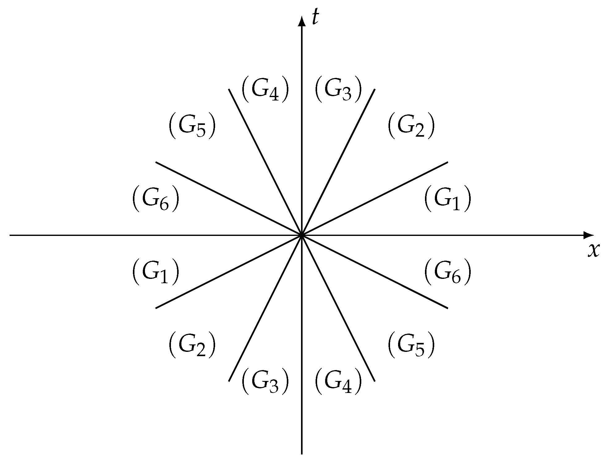
2.4. Jump Matrix

The spectral functions are shown to have a global relationship rather than being mutually independent. By utilizing [40], one can obtain the Riemann–Hilbert problem of the higher-order Gerdjikov–Ivanov equation.

To enable the subsequent computations, we introduce the following symbolic presumptions

$$\begin{array}{c}\phi \left(\beta \right)={\beta }^{2}z+2{\beta }^{6}t,\hfill \\ \gamma \left(\beta \right)=\overline{\chi \left(\overline{\beta }\right)}X\left(\beta \right)-\overline{k\left(\overline{\beta }\right)}K\left(\beta \right),\hfill \\ \omega \left(\beta \right)=\chi \left(\beta \right)K\left(\beta \right)-X\left(\beta \right)k\left(\beta \right),\hfill \\ \varrho \left(\beta \right)=\overline{\chi \left(\overline{\beta }\right)}\omega \left(\beta \right)+k\left(\beta \right)\gamma \left(\beta \right).\hfill \end{array}$$

The function $V(z,t;\beta )$ is defined as follows

$$\begin{array}{c}{V}_{+}(z,t,\beta )=({\displaystyle \frac{E_1^{G_1\cup G_2\cup G_3}(z,t,\beta )}{\overline{\gamma \left(\overline{\beta }\right)}}},E_3^{G_1\cup G_3}(z,t,\beta )),\beta \in G_1\cup G_3;\hfill \\ V_{-}(z,t,\beta )=({\displaystyle \frac{E_1^{G_1\cup G_2\cup G_3}(z,t,\beta )}{\chi \left(\beta \right)}},E_2^{G_2}(z,t,\beta )),\beta \in G_2;\hfill \\ V_{+}(z,t,\beta )=(E_2^{G_5}(z,t,\beta ),{\displaystyle \frac{E_1^{G_4\cup G_5\cup G_6}(z,t,\beta )}{\overline{\chi \left(\overline{\beta }\right)}}}),\beta \in G_5;\hfill \\ V_{-}(z,t,\beta )=(E_3^{G_4\cup G_6}(z,t,\beta ),{\displaystyle \frac{E_1^{G_4\cup G_5\cup G_6}(z,t,\beta )}{\gamma \left(\beta \right)}}),\beta \in G_4\cup G_6.\hfill \end{array}$$

(34)

These definitions mean that

$$\begin{array}{c}detV(z,t;\beta )=1,\\ V(z,t;\beta )=I+\mathcal{O}\left({\displaystyle \frac{1}{\beta }}\right),\beta \to \infty .\end{array}$$

Theorem 1. 

Consider that $u(z,t;\beta )$ is a smooth function, $V(z,t;\beta )$ is given by Equation (34), and $V(z,t;\beta )$ fulfills the jump relation

$$V_{+}(z,t,\beta )=V_{-}(z,t,\beta )L(z,t,\beta ),{\beta }^6\in \mathbb{R}.$$

(35)

where

$$L(z,t,\beta )=\left\{\begin{array}{cc}{L}_1(z,t,\beta ),\hfill & Arg\beta =k\pi ork\pi +{\displaystyle \frac{\pi }{2}};\hfill \\ L_2(z,t,\beta ),\hfill & Arg\beta =k\pi +{\displaystyle \frac{\pi }{6}}ork\pi +{\displaystyle \frac{\pi }{3}};\hfill \\ L_3(z,t,\beta ),\hfill & Arg\beta =k\pi +{\displaystyle \frac{2\pi }{3}}ork\pi +{\displaystyle \frac{5\pi }{6}}.\hfill \end{array}\right.$$

(36)

and

$$\begin{array}{c}{L}_1(z,t,\beta )=\left({\displaystyle \begin{array}{cc}\frac{1}{{\overline{\gamma \left(\overline{\beta }\right)}}^2}& \frac{\omega \left(\beta \right)}{\overline{\gamma \left(\overline{\beta }\right)}}{e}^{-2i\phi \left(\beta \right)}\\ -\frac{\gamma \left(\beta \right)\overline{\omega \left(\overline{\beta }\right)}}{{\overline{\gamma \left(\overline{\beta }\right)}}^2}{e}^{2i\phi \left(\beta \right)}& \frac{\gamma \left(\beta \right)}{\overline{\gamma \left(\overline{\beta }\right)}}\end{array}}\right),\hfill \\ L_2(z,t,\beta )=\left({\displaystyle \begin{array}{cc}\frac{\chi \left(\beta \right)}{\overline{\gamma \left(\overline{\beta }\right)}}& \frac{\chi \left(\beta \right)\varrho \left(\beta \right)}{\overline{\chi \left(\overline{\beta }\right)}}{e}^{-2i\phi \left(\beta \right)}\\ 0& \frac{\gamma \left(\beta \right)}{\overline{\chi \left(\overline{\beta }\right)}}\end{array}}\right),\hfill \\ L_3(z,t,\beta )=L_2{L}_1^{-1}{L}_4,\hfill \\ L_4(z,t,\beta )=\left({\displaystyle \begin{array}{cc}\frac{\chi \left(\beta \right)}{\overline{\chi \left(\overline{\beta }\right)}}& \frac{\chi \left(\beta \right)k\left(\beta \right)}{{\overline{\chi \left(\overline{\beta }\right)}}^2}{e}^{-2i\phi \left(\beta \right)}\\ -\frac{\overline{k\left(\overline{\beta }\right)}}{\overline{\chi \left(\overline{\beta }\right)}}{e}^{2i\phi \left(\beta \right)}& \frac{1}{{\overline{\chi \left(\overline{\beta }\right)}}^2}\end{array}}\right).\hfill \end{array}$$

The Riemann–Hilbert problem on the complex plane is depicted in Figure 5, with positive and negative values for each partition indicated.

Figure 5. There are positive and negative values for each partition on the complex $\beta$-plane.

Proof. 

We can express Equations (24), (25) and (29) in the form of a jump matrix, deriving the jump environment by expressing their relationship as follows:

$$\left\{\begin{array}{c}\overline{\chi \left(\overline{\beta }\right)}{E}_2^{G_5}+\overline{k\left(\overline{\beta }\right)}{e}^{2i\phi \left(\beta \right)}{E}_2^{G_2}=E_1^{G_1\cup G_2\cup G_3},\hfill \\ k\left(\beta \right)e^{-2i\phi \left(\beta \right)}{E}_2^{G_5}+\chi \left(\beta \right)E_2^{G_2}=E_1^{G_4\cup G_5\cup G_6},\hfill \end{array}\right.$$

(37)

$$\left\{\begin{array}{c}\overline{X\left(\overline{\beta }\right)}{E}_2^{G_3}+\overline{K\left(\overline{\beta }\right)}{e}^{2i\phi \left(\beta \right)}{E}_2^{G_2}=E_3^{G_4\cup G_6},\hfill \\ K\left(\beta \right)e^{-2i\phi \left(\beta \right)}{E}_2^{G_5}+X\left(\beta \right)E_2^{G_2}=E_3^{G_1\cup G_3},\hfill \end{array}\right.$$

(38)

$$\left\{\begin{array}{c}\begin{array}{c}\hfill (\chi \left(\beta \right)\overline{X\left(\overline{\beta }\right)}-k\left(\beta \right)\overline{K\left(\overline{\beta }\right)})E_1^{G_1\cup G_2\cup G_3}+e^{2i\phi \left(\beta \right)}(\overline{\chi \left(\overline{\beta }\right)}\overline{K\left(\overline{\beta }\right)}-\overline{k\left(\overline{\beta }\right)}\overline{X\left(\overline{\beta }\right)})E_1^{G_4\cup G_5\cup G_6}\\ \hfill =E_3^{G_4\cup G_6},\\ \hfill e^{-2i\phi \left(\beta \right)}(\chi \left(\beta \right)K\left(\beta \right)-X\left(\beta \right)k\left(\beta \right))E_1^{G_1\cup G_2\cup G_3}+(\overline{\chi \left(\overline{\beta }\right)}X\left(\beta \right)-\overline{k\left(\overline{\beta }\right)}K\left(\beta \right))E_1^{G_4\cup G_5\cup G_6}\\ \hfill =E_3^{G_1\cup G_3}.\end{array}\hfill \end{array}\right.$$

(39)

Equations (37)–(39) can be used to deduce that the jump matrices $L_i(z,t;\beta )(i=1,2,3,4.)$ fulfill

$$\begin{array}{c}\left({\displaystyle \frac{E_1^{G_1\cup G_2\cup G_3}(z,t,\beta )}{\overline{\gamma \left(\overline{\beta }\right)}},E_3^{G_1\cup G_3}(z,t,\beta )}\right)=\left({\displaystyle E_3^{G_4\cup G_6}(z,t,\beta ),\frac{E_1^{G_4\cup G_5\cup G_6}(z,t,\beta )}{\gamma \left(\beta \right)}}\right)L_1(z,t;\beta );\hfill \\ \left({\displaystyle \frac{E_1^{G_1\cup G_2\cup G_3}(z,t,\beta )}{\overline{\gamma \left(\overline{\beta }\right)}},E_3^{G_1\cup G_3}(z,t,\beta )}\right)=\left({\displaystyle \frac{E_1^{G_1\cup G_2\cup G_3}(z,t,\beta )}{\chi \left(\beta \right)},E_2^{G_2}(z,t,\beta )}\right)L_2(z,t;\beta );\hfill \\ \left({\displaystyle E_2^{G_5}(z,t,\beta ),\frac{E_1^{G_4\cup G_5\cup G_6}(z,t,\beta )}{\overline{\chi \left(\overline{\beta }\right)}}}\right)=\left({\displaystyle E_3^{G_4\cup G_6}(z,t,\beta ),\frac{E_1^{G_4\cup G_5\cup G_6}(z,t,\beta )}{\gamma \left(\beta \right)}}\right)L_3(z,t;\beta );\hfill \\ \left({\displaystyle E_2^{G_5}(z,t,\beta ),\frac{E_1^{G_4\cup G_5\cup G_6}(z,t,\beta )}{\overline{\chi \left(\overline{\beta }\right)}}}\right)=\left({\displaystyle \frac{E_1^{G_1\cup G_2\cup G_3}(z,t,\beta )}{\chi \left(\beta \right)},E_2^{G_2}(z,t,\beta )}\right)L_4(z,t;\beta ).\hfill \end{array}$$

(40)

This completes the proof. □

2.5. Residue Conditions

Hypothesis 1. 

Regarding functions $\gamma \left(\beta \right)$ and $\chi \left(\beta \right)$, we assume the following hypothesis:

(1) 

$\gamma \left(\beta \right)$ contains $2\nu$ simple zeros ${\left\{{\zeta }_j\right\}}_{j=1}^{2\nu }$($2\nu =2{\nu }_1+2{\nu }_2$). We assume that ${\zeta }_j$($j=1,2,\cdots ,2{\nu }_1$) pertains to $G_4\bigcup G_6$, and ${\overline{\zeta }}_j$($j=2{\nu }_1+1,2{\nu }_1+2,\cdots ,2\nu$) pertains to $G_1\bigcup G_3$.

(2) 

$\chi \left(\beta \right)$ contains $2\mu$ simple zeros ${\left\{{\epsilon }_j\right\}}_{j=1}^{2\mu }$ ($2\mu =2{\mu }_1+2{\mu }_2$). We assume that ${\epsilon }_j$( $j=1,2,\cdots ,2{\mu }_1$) pertains to $G_2$, and ${\overline{\epsilon }}_j$($j=2{\mu }_1+1,2{\mu }_1+2,\cdots ,2\mu$) pertains to $G_5$.

(3) 

There are distinctions between the simple zeros of $\gamma \left(\beta \right)$ and $\chi \left(\beta \right)$.

The Riemann–Hilbert problem is addressed by the solution denoted as ${\left[V(z,t;\beta )\right]}_1$ for the first column and ${\left[V(z,t;\beta )\right]}_2$ for the second column, which form the basis for subsequent propositions. Additionally, we write $\dot{\chi }\left(\beta \right)={\displaystyle \frac{d\chi }{d\beta }}$ and $\dot{\gamma }\left(\beta \right)={\displaystyle \frac{d\gamma }{d\beta }}$.

Proposition 4. 

(1) 

Res $\{{\left[V(z,t;\beta )\right]}_1,{\overline{\zeta }}_j\}$=${\displaystyle \frac{e^{2i\phi \left({\overline{\zeta }}_j\right)}}{\overline{\dot{\gamma }\left(\overline{{\zeta }_j}\right)}\omega \left({\overline{\zeta }}_j\right)}}{\left[V(z,t;{\overline{\zeta }}_j)\right]}_2$, $j=2{\nu }_1+1,2{\nu }_1+2,\cdots ,2\nu$.

(2) 

Res $\{{\left[V(z,t;\beta )\right]}_2,{\zeta }_j\}$=${\displaystyle \frac{e^{-2i\phi \left({\zeta }_j\right)}}{\dot{\gamma }\left({\zeta }_j\right)\overline{\omega \left(\overline{{\zeta }_j}\right)}}}{\left[V(z,t;{\zeta }_j)\right]}_1$, $j=1,2,\cdots ,2{\nu }_1$.

(3) 

Res $\{{\left[V(z,t;\beta )\right]}_1,{\epsilon }_j\}$=${\displaystyle \frac{e^{2i\phi \left({\epsilon }_j\right)}\overline{k\left({\overline{\epsilon }}_j\right)}}{\dot{\chi }\left({\epsilon }_j\right)}}{\left[V(z,t;{\epsilon }_j)\right]}_2$, $j=1,2,\cdots ,2{\mu }_1$.

(4) 

Res $\{{\left[V(z,t;\beta )\right]}_2,{\overline{\epsilon }}_j\}$=${\displaystyle \frac{e^{-2i\phi \left(\overline{{\epsilon }_j}\right)}k\left({\overline{\epsilon }}_j\right)}{\overline{\dot{\chi }\left({\overline{\epsilon }}_j\right)}}}{\left[V(z,t;{\overline{\epsilon }}_j)\right]}_1$, $j=2{\mu }_1+1,2{\mu }_1+2,\cdots ,2\mu$.

Proof. 

Let $V(z,t;\beta )=({\displaystyle \frac{E_1^{G_1\cup G_2\cup G_3}(z,t,\beta )}{\overline{\gamma \left(\overline{\beta }\right)}}},E_3^{G_1\cup G_3}(z,t,\beta ))$ be defined. The zeros $\overline{{\zeta }_j}$ ($j=2{\nu }_1+1,2{\nu }_1+2,\cdots ,2\nu$) of $\overline{\gamma \left(\overline{\beta }\right)}$ are the poles of ${\displaystyle \frac{E_1^{G_1\cup G_2\cup G_3}(z,t,\beta )}{\overline{\gamma \left(\overline{\beta }\right)}}}$. Next, we have

$$Res\{{\displaystyle \frac{E_1^{G_1\cup G_2\cup G_3}(z,t,\beta )}{\overline{\gamma \left(\overline{\beta }\right)}}},\overline{{\zeta }_j}\}=\underset{\beta \to \overline{{\zeta }_j}}{lim}(\beta -\overline{{\zeta }_j}){\displaystyle \frac{E_1^{G_1\cup G_2\cup G_3}(z,t,\beta )}{\overline{\gamma \left(\overline{\beta }\right)}}}={\displaystyle \frac{E_1^{G_1\cup G_2\cup G_3}(z,t;\overline{{\zeta }_j})}{\overline{\dot{\gamma }\left(\overline{{\zeta }_j}\right)}}}.$$

Substituting $\beta =\overline{{\zeta }_j}$ into the second equation of Equation (39) results in

$$E_1^{G_1\cup G_2\cup G_3}(z,t;\overline{{\zeta }_j})={\displaystyle \frac{1}{\omega \left({\overline{\zeta }}_j\right)}}{E}_3^{G_1\cup G_3}(z,t;\beta )e^{2i\phi \left({\overline{\zeta }}_j\right)}.$$

Furthermore,

$$Res\{{\displaystyle \frac{E_1^{G_1\cup G_2\cup G_3}(z,t;\beta )}{\overline{\gamma \left(\overline{\beta }\right)}}},{\overline{\zeta }}_j\}={\displaystyle \frac{e^{2i\phi \left({\overline{\zeta }}_j\right)}}{\overline{\dot{\gamma }\left(\overline{{\zeta }_j}\right)}\omega \left({\overline{\zeta }}_j\right)}}{E}_3^{G_1\cup G_3}(z,t;\beta ),$$

which can be calculated as (1).

Let $({\displaystyle \frac{E_1^{G_4\cup G_5\cup G_6}(z,t,\beta )}{\gamma \left(\beta \right)}},E_3^{G_4\cup G_6}(z,t,\beta ))$ be defined. The zeros ${\zeta }_j$ ($j=1,2,\cdots ,2{\nu }_1$) of $\gamma \left(\beta \right)$ are the poles of ${\displaystyle \frac{E_1^{G_4\cup G_5\cup G_6}(z,t,\beta )}{\gamma \left(\beta \right)}}$. Next, we have

$$Res\{{\displaystyle \frac{E_1^{G_4\cup G_5\cup G_6}(z,t,\beta )}{\gamma \left(\beta \right)}},{\zeta }_j\}=\underset{\beta \to {\zeta }_j}{lim}(\beta -{\zeta }_j){\displaystyle \frac{E_1^{G_4\cup G_5\cup G_6}(z,t;\beta )}{\gamma \left(\beta \right)}}={\displaystyle \frac{E_1^{G_4\cup G_5\cup G_6}(z,t;{\zeta }_j)}{\dot{\gamma }\left({\zeta }_j\right)}}.$$

Substituting $\beta ={\zeta }_j$ into the first equation of Equation (39) results in

$$E_1^{G_4\cup G_5\cup G_6}(z,t;{\zeta }_j)={\displaystyle \frac{E_3^{G_4\cup G_6}(z,t;{\zeta }_j)}{\overline{\omega \left({\overline{\zeta }}_j\right)}}}{e}^{-2i\phi \left({\zeta }_j\right)}.$$

Furthermore,

$$Res\{{\displaystyle \frac{E_1^{G_4\cup G_5\cup G_6}(z,t;\beta )}{\gamma \left(\beta \right)}},{\zeta }_j\}={\displaystyle \frac{e^{-2i\phi \left({\zeta }_j\right)}{E}_3^{G_4\cup G_6}(z,t;{\zeta }_j)}{\dot{\gamma }\left({\zeta }_j\right)\overline{\omega \left({\overline{\zeta }}_j\right)}}},$$

which can be calculated as (2).

Let $({\displaystyle \frac{E_1^{G_1\cup G_2\cup G_3}(z,t,\beta )}{\chi \left(\beta \right)}},E_2^{G_2}(z,t,\beta ))$ be defined. The zeros ${\epsilon }_j$ ($j=1,2,\cdots ,2{\mu }_1$) of $\chi \left(\beta \right)$ are the poles of ${\displaystyle \frac{E_1^{G_1\cup G_2\cup G_3}(z,t,\beta )}{\chi \left(\beta \right)}}$. Next, we have

$$Res\{{\displaystyle \frac{E_1^{G_1\cup G_2\cup G_3}(z,t,\beta )}{\chi \left(\beta \right)}},{\epsilon }_j\}=\underset{\beta \to {\epsilon }_j}{lim}(\beta -{\epsilon }_j){\displaystyle \frac{E_1^{G_1\cup G_2\cup G_3}(z,t,\beta )}{\chi \left(\beta \right)}}={\displaystyle \frac{E_1^{G_1\cup G_2\cup G_3}(z,t,{\epsilon }_j)}{\dot{\chi }\left({\epsilon }_j\right)}}.$$

Substituting $\beta ={\epsilon }_j$ into the second equation of Equation (37) results in

$$E_1^{G_1\cup G_2\cup G_3}(z,t,{\epsilon }_j)=\overline{k\left({\overline{\epsilon }}_j\right)}{e}^{2i\phi \left({\epsilon }_j\right)}{E}_2^{G_2}(z,t,{\epsilon }_j).$$

Furthermore,

$$Res\{{\displaystyle \frac{E_1^{G_1\cup G_2\cup G_3}(z,t,\beta )}{\chi \left(\beta \right)}},{\epsilon }_j\}={\displaystyle \frac{e^{2i\phi \left({\epsilon }_j\right)}\overline{k\left({\overline{\epsilon }}_j\right)}}{\dot{\chi }\left({\epsilon }_j\right)}}{E}_2^{G_2}(z,t,{\epsilon }_j),$$

which can be calculated as (3).

Let $(E_2^{G_5}(z,t,\beta ),{\displaystyle \frac{E_1^{G_4\cup G_5\cup G_6}(z,t,\beta )}{\overline{\chi \left(\overline{\beta }\right)}}})$ be defined. The zeros ${\overline{\epsilon }}_j$ ($j=2{\mu }_1+1,2{\mu }_1+2,\cdots ,2\mu$) of $\overline{\chi \left(\overline{\beta }\right)}$ are the poles of ${\displaystyle \frac{E_1^{G_4\cup G_5\cup G_6}(z,t,\beta )}{\overline{\chi \left(\overline{\beta }\right)}}}$. Next, we have

$$Res\{{\displaystyle \frac{E_1^{G_4\cup G_5\cup G_6}(z,t,\beta )}{\overline{\chi \left(\overline{\beta }\right)}}},{\overline{\epsilon }}_j\}=\underset{\beta \to {\overline{\epsilon }}_j}{lim}(\beta -{\overline{\epsilon }}_j){\displaystyle \frac{E_1^{G_4\cup G_5\cup G_6}(z,t;\beta )}{\overline{\chi \left(\overline{\beta }\right)}}}={\displaystyle \frac{E_1^{G_4\cup G_5\cup G_6}(z,t;{\overline{\epsilon }}_j)}{\overline{\dot{\chi }\left({\epsilon }_j\right)}}}.$$

Substituting $\beta ={\overline{\epsilon }}_j$ into the first equation of Equation (37) results in

$$E_1^{G_4\cup G_5\cup G_6}(z,t;{\overline{\epsilon }}_j)=E_2^{G_5}(z,t;\overline{{\epsilon }_j})k\left(\overline{{\epsilon }_j}\right)e^{-2i\phi \left({\overline{\epsilon }}_j\right)}.$$

Furthermore,

$$Res\{{\displaystyle \frac{{\mu }_1^{G_4\cup G_5\cup G_6}(z,t,\beta )}{\overline{\chi \left(\overline{\beta }\right)}}},{\overline{\epsilon }}_j\}={\displaystyle \frac{{\mu }_2^{G_5}(z,t;\overline{{\epsilon }_j})k\left(\overline{{\epsilon }_j}\right)e^{-2i\phi \left({\overline{\epsilon }}_j\right)}}{\overline{\dot{\chi }\left({\epsilon }_j\right)}}},$$

which can be calculated as (4). □

2.6. The Inverse Problem

Equation (34) representing the jump relation is equivalent to

$$V_{+}(z,t;\beta )-V_{-}(z,t;\beta )=V_{-}(z,t;\beta )L(z,t;\beta )-V_{-}(z,t;\beta ),$$

then

$$V_{+}(z,t;\beta )-V_{-}(z,t;\beta )=V_{-}\tilde{L}(z,t;\beta ),$$

(41)

where $\tilde{L}(z,t;\beta )=L(z,t;\beta )-I$. The function $V(z,t;\beta )$ is represented by its asymptotic expansion, as demonstrated below

$$V(z,t;\beta )=I+{\displaystyle \frac{\overline{V}(z,t;\beta )}{\beta }}+\mathcal{O}\left({\displaystyle \frac{1}{\beta }}\right),\beta \to \infty ,\beta \in \mathbb{C}\setminus \mathsf{\Gamma },$$

(42)

where $\mathsf{\Gamma }=\{{\beta }^6=\mathbb{R}\}$. The application of Equations (41) and (42) produces the following results

$$V(z,t;\beta )=I+{\displaystyle \frac{1}{2\pi i}}{\int }_{\mathsf{\Gamma }}{\displaystyle \frac{V_{+}(z,t;{\beta }^{\prime })\tilde{L}(z,t;{\beta }^{\prime })}{\beta -{\beta }^{\prime }}}d{\beta }^{\prime },\beta \in \mathbb{C}\setminus \mathsf{\Gamma },$$

(43)

and

$$\overline{V}(z,t;\beta )=-{\displaystyle \frac{1}{2\pi i}}{\int }_{\mathsf{\Gamma }}{V}_{+}(z,t;{\beta }^{\prime })\tilde{L}(z,t;{\beta }^{\prime })d{\beta }^{\prime }.$$

(44)

The reconstruction of the potential $u(z,t)$ from the spectral functions $E_k$, where $k=1,2,3$, is referred to as the inverse problem. Our objective is to reconstruct the potential $u(z,t)$. We need to think about $G_1^{\left(o\right)}$. As we demonstrate in Section 2.2 that

$$G_1^{\left(o\right)}=\left(\begin{array}{cc}0& -{\displaystyle \frac{i}{2}}u{G}_0^{22}\\ {\displaystyle \frac{i}{2}}v{G}_0^{11}& 0\end{array}\right),$$

when $\psi (z,t;\beta )=G_0+{\displaystyle \frac{G_1}{\beta }}+{\displaystyle \frac{G_2}{{\beta }^2}}+{\displaystyle \frac{G_3}{{\beta }^3}}+{\displaystyle \frac{G_4}{{\beta }^4}}+{\displaystyle \frac{G_5}{{\beta }^5}}+\mathcal{O}\left({\displaystyle \frac{1}{{\beta }^6}}\right)$, $(\beta \to \infty )$ is a result derived from Equation (18). From the formula above, we can derive

$$u(z,t)=2ig(z,t)e^{2i{\int }_{(0,0)}^{z,t}\Delta },$$

(45)

where

$$E(z,t;\beta )=I+{\displaystyle \frac{g_{12}^{\left(1\right)}(z,t;\beta )}{\beta }}+{\displaystyle \frac{g_{12}^{\left(2\right)}(z,t;\beta )}{{\beta }^2}}$$

$$+{\displaystyle \frac{g_{12}^{\left(3\right)}(z,t;\beta )}{{\beta }^3}}+{\displaystyle \frac{g_{12}^{\left(4\right)}(z,t;\beta )}{{\beta }^4}}+{\displaystyle \frac{g_{12}^{\left(5\right)}(z,t;\beta )}{{\beta }^5}}+\mathcal{O}\left({\displaystyle \frac{1}{{\beta }^6}}\right),(\beta \to \infty )$$

is the matching answer to Equation (18), which is linked to $\psi (z,t;\beta )$ through Equation (17). Through Equation (45) and its complex conjugate $v(z,t)$, we have

$$\begin{array}{c}uv={4\left|g\right|}^2,\hfill \\ u_z=2i{g}_z{e}^{2i{\int }_{(0,0)}^{z,t}\Delta }+4guv{e}^{2i{\int }_{(0,0)}^{z,t}\Delta },\hfill \\ v_z=-2i{\overline{g}}_z{e}^{-2i{\int }_{(0,0)}^{z,t}\Delta }+4\overline{g}uv{e}^{-2i{\int }_{(0,0)}^{z,t}\Delta },\hfill \\ u{v}_z-u_{z}v=4({\overline{g}}_{z}g-g_z\overline{g})+64i{\left|g\right|}^4.\hfill \end{array}$$

The inverse problem can be analyzed by following a three-step approach:

(1)

In the first step, we utilize $\psi (z,t;\beta )=G_0+{\displaystyle \frac{G_1}{\beta }}+{\displaystyle \frac{G_2}{{\beta }^2}}+{\displaystyle \frac{G_3}{{\beta }^3}}+{\displaystyle \frac{G_4}{{\beta }^4}}+{\displaystyle \frac{G_5}{{\beta }^5}}+\mathcal{O}\left({\displaystyle \frac{1}{{\beta }^6}}\right)$, $(\beta \to \infty )$ to compute $g(z,t)$ as

$$g(z,t)=\underset{\beta \to \infty }{lim}{\left(\beta E_k(z,t;\beta )\right)}_{12}.$$

(2)

In the second step, calculate $\Delta (z,t)$ by Equation (16).

(3)

In the third step, the expression for $u(z,t)$ is provided by Equation (45).

3. Definition and Properties of Spectral Functions and Riemann–Hilbert Problem

3.1. The Definition of Spectral Functions

Definition 1. 

(Regarding $\chi \left(\beta \right)$ and $k\left(\beta \right)$), we suppose that $u_0\left(z\right)=u(z,0)$, and define the map

$$\mathbb{S}:\left\{u_0\left(z\right)\right\}\to \{\chi \left(\beta \right),k\left(\beta \right)\},$$

where $\chi \left(\beta \right)$ and $k\left(\beta \right)$ are spectral functions.

$$\left(\begin{array}{c}k\left(\beta \right)\\ \chi \left(\beta \right)\end{array}\right)=E_1^{\left(2\right)}(z,0;\beta )=\left(\begin{array}{c}{E}_1^{12}(z,0;\beta )\\ E_1^{22}(z,0;\beta )\end{array}\right),\mathrm{Im}{\beta }^2\le 0,$$

where

$$E_1(z,0;\beta )=I+{\int }_{-\infty }^z{e}^{i{\beta }^2(\xi -z){\widehat{\theta }}_3}\left(B_1{E}_1\right)(\xi ,0;\beta )d\xi ,$$

and $B_1(z,0;\beta )$ is represented as follows

$$B_1(z,0;\beta )=\left(\begin{array}{cc}{\displaystyle \frac{i}{2}}{\left|u_0\right|}^2& \beta u_0{e}^{{\int }_0^{z}2i{\left|u_0\right|}^{2}d\xi }\\ \beta {\overline{u}}_0{e}^{-{\int }_0^{z}2i{\left|u_0\right|}^{2}d\xi }& -{\displaystyle \frac{i}{2}}{\left|u_0\right|}^2\end{array}\right).$$

Proposition 5. 

The following are the significant properties of $\chi \left(\beta \right)$ and $k\left(\beta \right)$

(1) 

For $\mathrm{Im}{\beta }^2\le 0$, $\chi \left(\beta \right)$ and $k\left(\beta \right)$ are all analytical;

(2) 

$\chi \left(\beta \right)=1+\mathcal{O}\left({\displaystyle \frac{1}{\beta }}\right),k\left(\beta \right)=\mathcal{O}\left({\displaystyle \frac{1}{\beta }}\right)$ as $\beta \to \infty$, $\mathrm{Im}{\beta }^2\le 0$;

(3) 

$\chi \left(\beta \right)\overline{\chi \left(\overline{\beta }\right)}-k\left(\beta \right)\overline{k\left(\overline{\beta }\right)}=1$, ${\beta }^2\in \mathbb{R}$;

(4) 

$\chi (-\beta )=\chi \left(\beta \right),k(-\beta )=-k\left(\beta \right)$, $\mathrm{Im}{\beta }^2\le 0$;

(5) 

${\mathbb{S}}^{-1}=\mathbb{Q}$, and the map $\mathbb{Q}:\{\chi \left(\beta \right),k\left(\beta \right)\}\to \left\{u_0\left(z\right)\right\}$, the maps $\mathbb{S}$ and $\mathbb{Q}$ are presented below

$$u_0\left(z\right)=2ig\left(z\right)e^{2i{\int }_0^z{\Delta }_1\left(\xi \right)d\xi },$$

$$g\left(z\right)=\underset{\beta \to \infty }{lim}{\left(\beta V^{\left(z\right)}(z,\beta )\right)}_{12},$$

where $V^{\left(z\right)}(z,\beta )$ acknowledges the given Riemann–Hilbert problem (see Theorem 1).

Proof. 

Numbers (1)–(5) follow from the discussion in Proposition 3. □

Theorem 2. 

Let

$$\begin{array}{c}{V}_{-}^{\left(z\right)}(z,\beta )=(E_2^{G_4\cup G_5\cup G_6}(z,\beta ),{\displaystyle \frac{E_1^{G_4\cup G_5\cup G_6}(z,\beta )}{\overline{\chi \left(\overline{\beta }\right)}}}),\mathrm{Im}{\beta }^2\le 0,\beta \in G_4\cup G_5\cup G_6,\hfill \\ V_{+}^{\left(z\right)}(z,\beta )=({\displaystyle \frac{E_1^{G_1\cup G_2\cup G_3}(z,\beta )}{\chi \left(\beta \right)}},E_2^{G_1\cup G_2\cup G_3}(z,\beta )),\mathrm{Im}{\beta }^2\ge 0,\beta \in G_1\cup G_2\cup G_3.\hfill \end{array}$$

(46)

$V^{\left(z\right)}(z,\beta )$ meets the Riemann–Hilbert problem as follows:

• $V^{\left(z\right)}(z,\beta )=\left\{\begin{array}{cc}{V}_{-}^{\left(z\right)}(z,\beta ),\hfill & \mathrm{Im}{\beta }^2\le 0\hfill \\ V_{+}^{\left(z\right)}(z,\beta ),\hfill & \mathrm{Im}{\beta }^2\ge 0\hfill \end{array}\right.$ is a piecewise analytic function.
• $V^{\left(z\right)}(z,\beta )$ fulfills asymptotic properties $V^{\left(z\right)}(z,\beta )=I+\mathcal{O}\left({\displaystyle \frac{1}{\beta }}\right),\beta \to \infty .$
• $V^{\left(z\right)}(z,\beta )$ meets the jump condition $V_{+}^{\left(z\right)}(z,\beta )=V_{-}^{\left(z\right)}(z,\beta )L^{\left(z\right)}(z,\beta )$, ${\beta }^2\in \mathbb{R}$
  where

  $$L^{\left(z\right)}(z,\beta )=\left(\begin{array}{cc}{\displaystyle \frac{1}{{\chi }^2\left(\beta \right)}}& -{\displaystyle \frac{k\left(\beta \right)}{\chi \left(\beta \right)}}{e}^{-2i{\beta }^{2}z}\\ {\displaystyle \frac{\overline{\chi \left(\overline{\beta }\right)k\left(\overline{\beta }\right)}}{{\chi }^2\left(\beta \right)}}{e}^{2i{\beta }^{2}z}& {\displaystyle \frac{\overline{\chi \left(\overline{\beta }\right)}}{\chi \left(\beta \right)}}\end{array}\right),{\beta }^2\in \mathbb{R}.$$

  (47)
• $\chi \left(\beta \right)$ contains $2\tilde{\mu }$ simple zeros ${\left\{{\epsilon }_j\right\}}_{j=1}^{2\tilde{\mu }}$ ($2\tilde{\mu }=2{\tilde{\mu }}_1+2{\tilde{\mu }}_2$). We assume that ${\epsilon }_j$( $j=1,2,\cdots ,2{\tilde{\mu }}_1$) belongs to $G_1\cup G_2\cup G_3$, and ${\overline{\epsilon }}_j$($j=2{\tilde{\mu }}_1+1,2{\tilde{\mu }}_1+2,\cdots ,2\tilde{\mu }$) belongs to $G_4\cup G_5\cup G_6$.
• The simple poles can be found at $\beta ={\overline{\epsilon }}_j$ ($j=2{\tilde{\mu }}_1+1,2{\tilde{\mu }}_1+2,\cdots ,2\tilde{\mu }$) in the second column of $V_{-}^{\left(z\right)}(z,\beta )$. The first column of $V_{+}^{\left(z\right)}(z,\beta )$ displays simple poles positioned at $\beta ={\epsilon }_j$ ($j=1,2,\cdots ,2{\tilde{\mu }}_1$).
  Then, the residue condition is

  $$Res\{{\left[V(z,t;\beta )\right]}_1,{\epsilon }_j\}={\displaystyle \frac{e^{2i{{\epsilon }_j}^{2}z}\overline{k\left({\overline{\epsilon }}_j\right)}}{\dot{\chi }\left({\epsilon }_j\right)}}{\left[V(z,t;{\epsilon }_j)\right]}_2,j=1,2,\cdots ,2{\tilde{\mu }}_1,$$

  (48)

  $$Res\{{\left[V(z,t;\beta )\right]}_2,{\overline{\epsilon }}_j\}={\displaystyle \frac{e^{-2i{\overline{\epsilon }}_j^{2}z}k\left({\overline{\epsilon }}_j\right)}{\overline{\dot{\chi }\left({\overline{\epsilon }}_j\right)}}}{\left[V(z,t;{\overline{\epsilon }}_j)\right]}_1,j=2{\tilde{\mu }}_1+1,2{\tilde{\mu }}_1+2,\cdots ,2\tilde{\mu }.$$

  (49)

Proof. 

According to Equation (38), we set $t=0$

$$\left\{\begin{array}{c}\overline{\chi \left(\overline{\beta }\right)}{E}_2^{G_4\cup G_5\cup G_6}+\overline{k\left(\overline{\beta }\right)}{e}^{2i{\beta }^{2}z}{E}_2^{G_1\cup G_2\cup G_3}=E_1^{G_1\cup G_2\cup G_3},\hfill \\ k\left(\beta \right)e^{-2i{\beta }^{2}z}{E}_2^{G_4\cup G_5\cup G_6}+\chi \left(\beta \right)E_2^{G_1\cup G_2\cup G_3}=E_1^{G_4\cup G_5\cup G_6}.\hfill \end{array}\right.$$

(50)

The jump matrix $L^{\left(z\right)}(z,\beta )$ satisfies the jump environment through calculation.

Take into account the first column of $V_{+}^{\left(z\right)}(z,\beta )$

$$Res\{{\displaystyle \frac{E_1^{G_1\cup G_2\cup G_3}(z,\beta )}{\chi \left(\beta \right)}},{\epsilon }_j\}=\underset{\beta \to {\epsilon }_j}{lim}(\beta -{\epsilon }_j){\displaystyle \frac{E_1^{G_1\cup G_2\cup G_3}(z,\beta )}{\chi \left(\beta \right)}}={\displaystyle \frac{E_1^{G_1\cup G_2\cup G_3}(z,{\epsilon }_j)}{\dot{\chi }\left({\epsilon }_j\right)}}.$$

By substituting $\beta ={\epsilon }_j$ into the second equation of Equation (50), we derive

$$E_1^{G_1\cup G_2\cup G_3}(z,{\epsilon }_j)=\overline{k\left({\overline{\epsilon }}_j\right)}{e}^{2i{{\epsilon }_j}^{2}z}{E}_2^{G_1\cup G_2\cup G_3}(z,{\epsilon }_j).$$

Furthermore,

$$Res\{{\displaystyle \frac{E_1^{G_1\cup G_2\cup G_3}(z,\beta )}{\chi \left(\beta \right)}},{\epsilon }_j\}={\displaystyle \frac{e^{2i{{\epsilon }_j}^{2}z}\overline{k\left({\overline{\epsilon }}_j\right)}}{\dot{\chi }\left({\epsilon }_j\right)}}{\left[M(z,t;{\epsilon }_j)\right]}_2,j=1,2,···,2{\tilde{\mu }}_1.$$

It can be considered the same as Equation (48). We can demonstrate that Equation (49) holds by applying the same method. □

Definition 2. 

(Regarding $X\left(\beta \right)$ and $K\left(\beta \right)$), we suppose that $f_0\left(t\right)$, $f_1\left(t\right)$, and define the map

$$\tilde{\mathbb{S}}:\{f_0\left(t\right),f_1\left(t\right)\}\to \{X\left(\beta \right),K\left(\beta \right)\}$$

where $X\left(\beta \right)$ and $K\left(\beta \right)$ are spectral functions.

$$\left(\begin{array}{c}K\left(\beta \right)\\ X\left(\beta \right)\end{array}\right)=E_3^{\left(2\right)}(0,\beta )=\left(\begin{array}{c}{E}_3^{12}(0,\beta )\\ E_3^{22}(0,\beta )\end{array}\right),Im{\beta }^6\ge 0,$$

where

$$E_3(0,\beta )=I-{\int }_t^T{e}^{2i{\beta }^6(\tau -T){\widehat{\theta }}_3}\left(B_2{E}_3\right)(0,\tau ,\beta )d\tau ,$$

and $B_2(0,t;\beta )$ is represented as follows

$$\begin{array}{c}{B}_2(0,t;\beta )=\left(\begin{array}{cc}{B}_2^{11}(0,t;\beta )& B_2^{12}(0,t;\beta )\\ B_2^{21}(0,t;\beta )& B_2^{22}(0,t;\beta )\end{array}\right).\hfill \\ B_2^{11}=-i{\beta }^4|f_0{|}^2-{\displaystyle \frac{1}{2}}{\beta }^2(f_0{\overline{f}}_1-f_1{\overline{f}}_0)+{\displaystyle \frac{i}{4}}{\beta }^2|f_0{|}^4-{\displaystyle \frac{i}{4}}{f}_2{\overline{f}}_0-{\displaystyle \frac{i}{4}}{f}_0{\overline{f}}_2+{\displaystyle \frac{i}{4}}|f_1{|}^2+{\displaystyle \frac{3}{8}}i{\left|f_0\right|}^6,\hfill \\ B_2^{12}=(2{\beta }^5{f}_0+i{\beta }^3{f}_1-{\displaystyle \frac{1}{2}}\beta f_2-{\displaystyle \frac{i}{2}}\beta f_0^2{\overline{f}}_1-{\displaystyle \frac{1}{4}}\beta f_0^3{\overline{f}}_0^2)e^{-2i{\int }_0^t{\Delta }_2(0,\tau )d\tau },\hfill \\ B_2^{21}=(2{\beta }^5{\overline{f}}_0-i{\beta }^3{\overline{f}}_1-{\displaystyle \frac{1}{2}}\beta {\overline{f}}_2+{\displaystyle \frac{i}{2}}\beta f_1{\overline{f}}_0^2-{\displaystyle \frac{1}{4}}\beta f_0^2{\overline{f}}_0^3)e^{2i{\int }_0^t{\Delta }_2(0,\tau )d\tau },\hfill \\ B_2^{22}=i{\beta }^4|f_0{|}^2-{\displaystyle \frac{1}{2}}{\beta }^2(f_1{\overline{f}}_0-f_0{\overline{f}}_1)-{\displaystyle \frac{i}{4}}{\beta }^2|f_0{|}^4+{\displaystyle \frac{i}{4}}{f}_2{\overline{f}}_0+{\displaystyle \frac{i}{4}}{f}_0{\overline{f}}_2-{\displaystyle \frac{i}{4}}|f_1{|}^2-{\displaystyle \frac{3}{8}}i{|f_0|}^6,\hfill \end{array}$$

where ${\Delta }_2(0,\tau )=-{\displaystyle \frac{1}{2}}{f}_2{\overline{f}}_0+{\displaystyle \frac{1}{2}}{f}_0{\overline{f}}_2-{\displaystyle \frac{1}{2}}|f_1{|}^2-{\displaystyle \frac{1}{4}}{|f_0|}^6$.

Proposition 6. 

The following are the significant properties of the $X\left(\beta \right)$ and $K\left(\beta \right)$.

(1) 

For $\mathrm{Im}{\beta }^6>0$, $X\left(\beta \right)$ and $K\left(\beta \right)$ are analytical;

(2) 

$X\left(\beta \right)=1+\mathcal{O}\left({\displaystyle \frac{1}{\beta }}\right),K\left(\beta \right)=\mathcal{O}\left({\displaystyle \frac{1}{\beta }}\right)$ as $\beta \to \infty$, $\mathrm{Im}{\beta }^6\ge 0$;

(3) 

$X\left(\beta \right)\overline{X\left(\overline{\beta }\right)}-K\left(\beta \right)\overline{K\left(\overline{\beta }\right)}=1$, ${\beta }^6\in \mathbb{R}$;

(4) 

$X(-\beta )=X\left(\beta \right),K(-\beta )=-K\left(\beta \right)$, $\mathrm{Im}{\beta }^6\ge 0$;

(5) 

${\tilde{\mathbb{S}}}^{-1}=\tilde{\mathbb{Q}}$, and the map $\tilde{\mathbb{Q}}:\{X\left(\beta \right),K\left(\beta \right)\}\to \{f_0\left(t\right),f_1\left(t\right),f_2\left(t\right)\}$, the maps $\mathbb{S}$ of $\mathbb{Q}$ are presented below:

$$f_0\left(t\right)=2i{g}^{\left(1\right)}\left(t\right)e^{2i{\int }_0^t{\Delta }_2\left(\tau \right)d\tau },$$

(51)

where the function $g^{\left(1\right)}\left(t\right)$ fullfills the given relationship $V^{\left(t\right)}(t,\beta )=I+{\displaystyle \frac{g^{\left(1\right)}(t,\beta )}{\beta }}+\mathcal{O}\left({\displaystyle \frac{1}{\beta }}\right),$$(\beta \to \infty )$ and $V^{\left(t\right)}(t,\beta )$ meets the following Riemann–Hilbert problem (see Theorem 2).

Proof. 

Numbers (1)–(5) follow from the discussion in Proposition 3. □

Theorem 3. 

Let

$$\begin{array}{c}{V}_{-}^{\left(t\right)}(t,\beta )=(E_3^{G_2\cup G_4\cup G_6}(t,\beta ),{\displaystyle \frac{E_2^{G_2\cup G_4\cup G_6}(t,\beta )}{\overline{X\left(\overline{\beta }\right)}}}),\mathrm{Im}{\beta }^6\le 0,\beta \in G_2\cup G_4\cup G_6,\hfill \\ \\ V_{+}^{\left(t\right)}(t,\beta )=({\displaystyle \frac{E_2^{G_1\cup G_3\cup G_5}(t,\beta )}{X\left(\beta \right)}},E_3^{G_1\cup G_3\cup G_5}(t,\beta )),\mathrm{Im}{\beta }^6\ge 0,\beta \in G_1\cup G_3\cup G_5.\hfill \end{array}$$

(52)

$V^{\left(t\right)}(t,\beta )$ meets the Riemann–Hilbert problem as follows:

• $V^{\left(t\right)}(t,\beta )=\left\{\begin{array}{cc}{V}_{-}^{\left(t\right)}(t,\beta ),\hfill & \mathrm{Im}{\beta }^6\le 0\hfill \\ V_{+}^{\left(t\right)}(t,\beta ),\hfill & \mathrm{Im}{\beta }^6\ge 0\hfill \end{array}\right.$ is a piecewise analytic function.
• $V^{\left(t\right)}(t,\beta )$ fulfills asymptotic properties $V^{\left(t\right)}(t,\beta )=I+\mathcal{O}\left({\displaystyle \frac{1}{\beta }}\right),\beta \to \infty .$
• $V^{\left(t\right)}(t,\beta )$ meets the jump condition $V_{+}^{\left(t\right)}(t,\beta )=V_{-}^{\left(t\right)}(t,\beta )L^{\left(t\right)}(t,\beta )$, ${\beta }^6\in \mathbb{R}$
  where

  $$L^{\left(t\right)}(t,\beta )=\left(\begin{array}{cc}{\displaystyle \frac{1}{X\left(\beta \right)\overline{X\left(\overline{\beta }\right)}}}& {\displaystyle \frac{K\left(\beta \right)}{\overline{X\left(\overline{\beta }\right)}}}{e}^{-4i{\beta }^{6}t}\\ -{\displaystyle \frac{\overline{K\left(\overline{\beta }\right)}}{X\left(\beta \right)}}{e}^{4i{\beta }^{6}t}& 1\end{array}\right),{\beta }^6\in \mathbb{R}.$$

  (53)
• $X\left(\beta \right)$ contains $2k$ simple zeros ${\left\{{\kappa }_j\right\}}_1^{2n}$ ($2n=2n_1+2n_2$). We assume that ${\kappa }_j$($j=1,2,\cdots ,2n_1$) belongs to $G_1\bigcup G_3\bigcup G_5$, and ${\overline{\kappa }}_j$($j=2n_1+1,2n_1+2,\cdots ,2n$) belongs to $G_2\bigcup G_4\bigcup G_6$.
• The simple poles can be found at $\beta ={\kappa }_j$ ($j=1,2,\cdots ,2n_1$) in the first column of $V_{+}^{\left(t\right)}(t,\beta )$. The second column of $V_{-}^{\left(t\right)}(t,\beta )$ displays simple poles positioned at $\beta ={\overline{\kappa }}_j$($j=2n_1+1,2n_1+2,\cdots ,2n$).
  Then, the residue condition is

  $$Res\{{\left[V^{\left(t\right)}(t,\beta )\right]}_1,{\kappa }_j\}={\displaystyle \frac{e^{4i{\kappa }_j^{6}t}}{\dot{X}\left({\kappa }_j\right)K\left({\kappa }_j\right)}}{\left[V^{\left(t\right)}(t,{\kappa }_j)\right]}_2,j=1,2,\cdots ,2n_1,$$

  (54)

  $$Res\{{\left[V^{\left(t\right)}(t,\beta )\right]}_2,{\overline{\kappa }}_j\}={\displaystyle \frac{e^{-4i{\kappa }_j^{6}t}}{\overline{\dot{X}\left({\overline{\kappa }}_j\right)}\overline{K\left({\overline{\kappa }}_j\right)}}}{\left[V^{\left(t\right)}(t,{\overline{\kappa }}_j)\right]}_1,j=2n_1+1,2n_1+2,\cdots ,2n.$$

  (55)

Proof. 

According to Equation (39), we set $z=0$

$$\left\{\begin{array}{c}\overline{X\left(\overline{\beta }\right)}{E}_2^{G_1\cup G_3\cup G_5}+\overline{K\left(\overline{\beta }\right)}{e}^{4i{\beta }^{6}t}{E}_2^{G_2\cup G_4\cup G_6}=E_3^{G_2\cup G_4\cup G_6},\hfill \\ K\left(\beta \right)e^{-4i{\beta }^{6}t}{E}_2^{G_1\cup G_3\cup G_5}+X\left(\beta \right)E_2^{G_2\cup G_4\cup G_6}=E_3^{G_1\cup G_3\cup G_5}.\hfill \end{array}\right.$$

(56)

The jump matrix $L^{\left(t\right)}(t,\beta )$ satisifies the jump environment through calculation.

Take into account the first column of $V_{+}^{\left(t\right)}(t,\beta )$

$$Res\{{\displaystyle \frac{E_2^{G_1\cup G_3\cup G_5}(t,\beta )}{X\left(\beta \right)}},{\kappa }_j\}=\underset{\beta \to {\kappa }_j}{lim}(\beta -{\kappa }_j){\displaystyle \frac{E_2^{G_1\cup G_3\cup G_5}(t,\beta )}{X\left(\beta \right)}}={\displaystyle \frac{E_2^{G_1\cup G_3\cup G_5}(t,{\kappa }_j)}{\dot{X}\left({\kappa }_j\right)}}.$$

By substituting $\beta ={\kappa }_j$ into the second equation of Equation (55), we derive

$$E_2^{G_1\cup G_3\cup G_5}(t,{\kappa }_j)={\displaystyle \frac{1}{K\left({\kappa }_j\right)}}{e}^{4i{{\kappa }_j}^{6}t}{E}_3^{G_1\cup G_3\cup G_5}(t,{\kappa }_j).$$

Furthermore,

$$Res\{{\displaystyle \frac{E_2^{G_1\cup G_3\cup G_5}(t,\beta )}{X\left(\beta \right)}},{\kappa }_j\}={\displaystyle \frac{e^{4i{\kappa }_j^{6}t}}{\dot{X}\left({\kappa }_j\right)K\left({\kappa }_j\right)}}{\left[M^{\left(t\right)}(t,{\kappa }_j)\right]}_2,j=1,2,\cdots ,2n_1.$$

It can be considered the same as Equation (54). We can demonstrate that Equation (55) holds by applying the same method. □

Definition 3. 

(Regarding $\gamma \left(\beta \right)$ and $\omega \left(\beta \right)$), we suppose that

$$\gamma \left(\beta \right)=\overline{s\left(\overline{\beta }\right)}S\left(\beta \right)-\overline{k\left(\overline{\beta }\right)}K\left(\beta \right),\omega \left(\beta \right)=s\left(\beta \right)K\left(\beta \right)-k\left(\beta \right)S\left(\beta \right),$$

and the smooth functions $u_T\left(z\right)=u(z,T)$. We define the map

$$\widetilde{\tilde{\mathbb{S}}}:\left\{u_T\left(z\right)\right\}\to \{\gamma \left(\beta \right),\omega \left(\beta \right)\}$$

by

$$\left(\begin{array}{c}\omega \left(\beta \right)\\ \gamma \left(\beta \right)\end{array}\right)=E_3^{\left(2\right)}(0,\beta )=\left(\begin{array}{c}{E}_3^{12}(0,\beta )\\ E_3^{22}(0,\beta )\end{array}\right),Im{\beta }^2\ge 0,$$

where

$$E_3(z,T;\beta )=I-{\int }_z^0{e}^{i{\beta }^2(\xi -x){\widehat{\sigma }}_3}\left(B_1{E}_3\right)(\xi ,T;\beta )d\xi ,$$

$$E_1(z,T;\beta )=I+{\int }_{-\infty }^z{e}^{i{\beta }^2(\xi -x){\widehat{\sigma }}_3}\left(B_1{E}_1\right)(\xi ,T;\beta )d\xi ,$$

and $B_1(z,T;\beta )$ is represented as follows

$$B_1(z,T;\beta )=\left(\begin{array}{cc}{\displaystyle \frac{i}{2}}{\left|f_T\right|}^2& \beta f_T{e}^{{\int }_0^{z}2i{\left|f_T\right|}^{2}d\xi }\\ \beta {\overline{f}}_T{e}^{-{\int }_0^{z}2i{\left|f_T\right|}^{2}d\xi }& -{\displaystyle \frac{i}{2}}{\left|f_T\right|}^2\end{array}\right).$$

Proposition 7. 

The following are the significant properties of the $\gamma \left(\beta \right)$ and $\omega \left(\beta \right)$.

(1) 

For $\mathrm{Im}{\beta }^2\ge 0$, $\gamma \left(\beta \right)$ and $\omega \left(\beta \right)$ are analytical;

(2) 

$\gamma \left(\beta \right)=1+\mathcal{O}\left({\displaystyle \frac{1}{\beta }}\right),\omega \left(\beta \right)=\mathcal{O}\left({\displaystyle \frac{1}{\beta }}\right)$ as $\beta \to \infty$, $\mathrm{Im}{\beta }^2\ge 0$;

(3) 

$\gamma \left(\beta \right)\overline{\gamma \left(\overline{\beta }\right)}-\omega \left(\beta \right)\overline{\omega \left(\overline{\beta }\right)}=1$, ${\beta }^2\in \mathbb{R}$;

(4) 

$\gamma (-\beta )=\gamma \left(\beta \right),\omega (-\beta )=-\omega \left(\beta \right)$, $\mathrm{Im}{\beta }^2\ge 0$;

(5) 

${\widetilde{\tilde{\mathbb{S}}}}^{-1}=\widetilde{\tilde{\mathbb{Q}}}$, and the map $\widetilde{\tilde{\mathbb{Q}}}:\{\gamma \left(\beta \right),\omega \left(\beta \right)\}\to \left\{f_T\left(z\right)\right\}$, the maps $\widetilde{\tilde{\mathbb{S}}}$ and $\widetilde{\tilde{\mathbb{Q}}}$ are presented below

$$f_T\left(z\right)=2i{g}_T\left(z\right)e^{2i{\int }_z^0{\Delta }_1(\xi ,T)d\xi },$$

(57)

$$g_T\left(z\right)=\underset{\beta \to \infty }{lim}{\left(\beta V^{\left(T\right)}(z,\beta )\right)}_{12},$$

(58)

where $V^{\left(T\right)}(z,\beta )$ satisfies the given Riemann–Hilbert problem (see Theorem 3).

Proof. 

Numbers (1)–(5) follow from the discussion in Proposition 3. □

Theorem 4. 

Let

$$\begin{array}{c}{V}_{-}^{\left(T\right)}(z,T,\beta )=(E_3^{G_4\cup G_5\cup G_6}(z,T,\beta ),{\displaystyle \frac{E_1^{G_4\cup G_5\cup G_6}(z,T,\beta )}{\gamma \left(\beta \right)}}),\mathrm{Im}{\beta }^2\le 0,\beta \in G_4\cup G_5\cup G_6,\hfill \\ V_{+}^{\left(T\right)}(z,T,\beta )=({\displaystyle \frac{E_1^{G_1\cup G_2\cup G_3}(z,T,\beta )}{\overline{\gamma \left(\overline{\beta }\right)}}},E_3^{G_1\cup G_2\cup G_3}(z,T,\beta )),\mathrm{Im}{\beta }^2\ge 0,\beta \in G_1\cup G_2\cup G_3.\hfill \end{array}$$

(59)

$V^{\left(T\right)}(z,\beta )$ meets the Riemann–Hilbert problem as follows:

• $V^{\left(T\right)}(z,\beta )=\left\{\begin{array}{cc}{V}_{-}^{\left(T\right)}(z,\beta ),\hfill & \mathrm{Im}{\beta }^2\le 0\hfill \\ V_{+}^{\left(T\right)}(z,\beta ),\hfill & \mathrm{Im}{\beta }^2\ge 0\hfill \end{array}\right.$ is a piecewise analytic function.
• $V^{\left(T\right)}(z,\beta )$ fulfills asymptotic properties $V^{\left(T\right)}(z,\beta )=I+\mathcal{O}\left({\displaystyle \frac{1}{\beta }}\right),\beta \to \infty .$
• $V^{\left(z\right)}(z,\beta )$ meets the jump condition $V_{+}^{\left(T\right)}(z,\beta )=V_{-}^{\left(T\right)}(z,\beta )L^{\left(T\right)}(z,\beta )$, ${\beta }^2\in \mathbb{R}$,
  where

  $$L^{\left(T\right)}(z,\beta )=\left(\begin{array}{cc}{\displaystyle \frac{1}{{\overline{\gamma \left(\overline{\beta }\right)}}^2}}& {\displaystyle \frac{\omega \left(\beta \right)}{\overline{\gamma \left(\overline{\beta }\right)}}}{e}^{-2i({\beta }^{2}z+2{\beta }^{6}T)}\\ -{\displaystyle \frac{\gamma \left(\beta \right)\overline{\omega \left(\overline{\beta }\right)}}{{\overline{\gamma \left(\overline{\beta }\right)}}^2}}{e}^{2i({\beta }^{2}z+2{\beta }^{6}T)}& {\displaystyle \frac{\gamma \left(\beta \right)}{\overline{\gamma \left(\overline{\beta }\right)}}}\end{array}\right),{\beta }^2\in \mathbb{R}.$$

  (60)
• $\gamma \left(\beta \right)$ contains $2\tilde{\mu }$ simple zeros ${\left\{{\nu }_j\right\}}_{j=1}^{2\tilde{\mu }}$($2\tilde{\mu }=2{\tilde{\mu }}_1+2{\tilde{\mu }}_2$). We assume that ${\nu }_j$($j=1,2,\cdots ,2{\tilde{\mu }}_1$) belongs to $G_1\bigcup G_2\bigcup G_3$, and ${\overline{\nu }}_j$($j=2{\tilde{\mu }}_1+1,2{\tilde{\mu }}_1+2,\cdots ,2\tilde{\mu }$) belongs to $G_4\bigcup G_5\bigcup G_6$.
• The simple poles can be found at $\beta ={\nu }_j$ ($j=1,2,\cdots ,2{\tilde{\mu }}_1$) in the first column of $V_{+}^{\left(T\right)}(z,\beta )$. The second column of $V_{-}^{\left(T\right)}(z,\beta )$ displays simple pole positions at $\beta ={\overline{\nu }}_j$( $j=2{\tilde{\mu }}_1+1,2{\tilde{\mu }}_1+2,\cdots ,2\tilde{\mu }$).
  Then, the residue condition is

  $$Res\{{\left[V^{\left(T\right)}(z,\beta )\right]}_1,{\nu }_j\}={\displaystyle \frac{e^{2i({\nu }_j^{2}z+2{\nu }_j^{6}T)}}{\overline{\dot{\gamma }\left({\overline{\nu }}_j\right)}\omega \left({\nu }_j\right)}}{\left[V^{\left(T\right)}(z,{\nu }_j)\right]}_2,j=1,2,\cdots ,2{\tilde{\mu }}_1,$$

  (61)

  $$Res\{{\left[V^{\left(T\right)}(z,\beta )\right]}_2,{\overline{\nu }}_j\}={\displaystyle \frac{e^{-2i({\nu }_j^{2}z+2{\nu }_j^{6}T)}}{\dot{\gamma }\left({\overline{\nu }}_j\right)\overline{\omega \left(\overline{{\nu }_j}\right)}}}{\left[V^{\left(T\right)}(z,{\overline{\gamma }}_j)\right]}_1,j=2{\tilde{\mu }}_1+1,2{\tilde{\mu }}_1+2,\cdots ,2\tilde{\mu }.$$

  (62)

Proof. 

According to Equation (39), we set $t=L$

$$\left\{\begin{array}{c}\overline{\gamma \left(\overline{\beta }\right)}{E}_1^{G_1\cup G_2\cup G_3}+e^{2i\theta \left(\beta \right)}\overline{\omega \left(\overline{\beta }\right)}{E}_1^{G_4\cup G_5\cup G_6}=E_3^{G_4\cup G_5\cup G_6},\hfill \\ e^{-2i\theta \left(\beta \right)}\omega \left(\beta \right)E_1^{G_1\cup G_2\cup G_3}+\gamma \left(\beta \right)E_1^{G_4\cup G_5\cup G_6}=E_3^{G_1\cup G_2\cup G_3}.\hfill \end{array}\right.$$

(63)

The jump matrix $L^{\left(z\right)}(z,\beta )$ satisfies the jump environment through calculation.

Take into account the first column of $V_{+}^{\left(z\right)}(z,\beta )$

$$Res\{{\displaystyle \frac{E_1^{G_1\cup G_2\cup G_3}(z,\beta )}{\overline{\gamma \left(\overline{\beta }\right)}}},{\nu }_j\}=\underset{\beta \to {\nu }_j}{lim}(\beta -{\nu }_j){\displaystyle \frac{E_1^{G_1\cup G_2\cup G_3}(z,\beta )}{\overline{\gamma \left(\overline{\beta }\right)}}}={\displaystyle \frac{E_1^{G_1\cup G_2\cup G_3}(z,{\nu }_j)}{\overline{\dot{\gamma }\left(\overline{{\nu }_j}\right)}}}.$$

By substituting $\beta ={\nu }_j$ into the second equation of Equation (59), we derive

$$E_1^{G_1\cup G_2\cup G_3}(z,{\nu }_j)={\displaystyle \frac{1}{\omega \left({\nu }_j\right)}}{e}^{2i({\nu }_j^{2}z+{\nu }_j^{6}L)}{E}_3^{G_1\cup G_2\cup G_3}(z,{\nu }_j).$$

Furthermore,

$$Res\{{\displaystyle \frac{E_1^{G_1\cup G_2\cup G_3}(z,\beta )}{\overline{\gamma \left(\overline{\beta }\right)}}},{\nu }_j\}={\displaystyle \frac{e^{2i({\nu }_j^{2}z+{\nu }_j^{6}L)}}{\overline{\dot{\gamma }\left(\overline{{\nu }_j}\right)}\omega \left({\nu }_j\right)}}{\left[M^{\left(t\right)}(t,{\kappa }_j)\right]}_2,j=1,2,\cdots ,2{\tilde{\mu }}_1.$$

It can be considered the same as Equation (61). We can demonstrate that Equation (62) holds by applying the same method. □

3.2. Riemann–Hilbert Problem

Theorem 5. 

The matrix functions $s_1\left(\beta \right)$ and $s_2\left(\beta \right)$ are defined by $\chi \left(\beta \right)$, $k\left(\beta \right)$, $X\left(\beta \right)$, and $K\left(\beta \right)$, respectively. The spectral functions $u_0\left(z\right)$, $f_0\left(t\right)$, and $f_1\left(t\right)$ of Definitions 1 and 2 indicate $\chi \left(\beta \right)$, $k\left(\beta \right)$, $X\left(\beta \right),$ and $K\left(\beta \right)$. Suppose that $\chi \left(\beta \right)$, $k\left(\beta \right)$, $X\left(\beta \right)$, and $K\left(\beta \right)$ satisfy the global relation.

$$\chi \left(\beta \right)K\left(\beta \right)-k\left(\beta \right)X\left(\beta \right)=e^{4i{\beta }^{6}T}{b}^{+}\left(\beta \right),Im{\beta }^6\ge 0,$$

where $b^{+}\left(\beta \right)$ is an entire function. $s_1\left(\beta \right)=E_1(0,0;\beta )$, $s_2\left(\beta \right)=s_2(T,\beta )={\left(e^{2i{\beta }^{6}T}{E}_2(0,T;\beta )\right)}^{-1}$. The global relation is transformed into $\chi \left(\beta \right)K\left(\beta \right)-k\left(\beta \right)X\left(\beta \right)=0$ if $\beta \to \infty$. Define the $V(z,t,\beta )$ as the answer to the subsequent $2\times 2$ Riemann–Hilbert problem.

• The function $V(z,t;\beta )$ is an analytical function that acts upon sections and has a unit determinant.
• $V(z,t;\beta )$ meets the jump condition

  $$V_{+}(z,t;\beta )=V_{-}(z,t;\beta )L(z,t;\beta ),{\beta }^6\in \mathbb{R}.$$

  (64)
• The simple poles can be found at $\beta ={\zeta }_j$ ($j=1,2,\cdots ,2{\nu }_1$) and $\beta ={\overline{\epsilon }}_j$ ($j=2{\mu }_1+1,2{\mu }_1+2,\cdots ,2\mu$) in the second column of $V(z,t;\beta )$. Simple poles can also be found at $\beta ={\overline{\zeta }}_j$ ($j=2{\nu }_1+1,2{\nu }_1+2,\cdots ,2\nu$) and $\beta ={\epsilon }_j$( $j=1,2,\cdots ,2{\mu }_1$) in the first column of $V(z,t;\beta )$.
• $V(z,t;\beta )=I+\mathcal{O}\left({\displaystyle \frac{1}{\beta }}\right),\beta \to \infty$.
• Hypothesis 1 illustrates the residual relationship that $V(z,t;\beta )$ possesses.

Then, the function $V(z,t;\beta )$ both exists and is unique.

Given $V(z,t;\beta )$, define $u(z,t)$ as

$$\begin{array}{c}u(z,t)=2ig(z,t)e^{2i{\int }_{(0,0)}^{(z,t)}\Delta },\hfill \\ g(z,t)=\underset{\beta \to \infty }{lim}{\left(\beta V(z,t;\beta )\right)}_{12}.\hfill \end{array}$$

(65)

Then, we can obtain $u(z,t)$, which represents the solution to the higher-order Gerdjikov–Ivanov equation Equation (4), with initial boundary conditions $u(z,0)=u_0\left(z\right)$, $u(0,t)=f_0\left(t\right)$, $u_z(0,t)=f_1\left(t\right)$, and $u_{zz}(0,t)=f_2\left(t\right)$.

Proof. 

If $s_1\left(\beta \right)$ and $s_2\left(\beta \right)$ do not have any zeros, it can be assumed that the $(2\times 2)$ function $V(z,t;\beta )$ adheres to a non-singular Riemann–Hilbert problem. By utilizing the correspondence between the jump matrix $L(z,t,\beta )$ and symmetry conditions, it is possible to demonstrate that this problem has a global solution. The scenario where $s_1\left(\beta \right)$ and $s_2\left(\beta \right)$ have a limited number of zeros can be transformed into an equivalent situation with no zeros by introducing an algebraic system of equations that always has a solvable outcome. □

Theorem 6. 

Given the vanishing boundary condition $V(z,t;\beta )\to 0$ ($\beta \to \infty )$, Theorem 5 states that there is only zero solution to the Riemann–Hilbert problem.

Proof. 

Assuming that $V_{\pm }(z,t;\beta )\to \infty$ ($\beta \to \infty )$ represents a proposed resolution to the Riemann–Hilbert problem as stated in Theorem 6, suppose that $𝘍$ denotes a $2\times 2$ matrix. The symbol used to represent the complex conjugate transpose of $𝘍$ is ${𝘍}^{†}$.

Provide a definition

$$\begin{array}{c}{\varkappa }_{+}\left(\beta \right)=V_{+}\left(\beta \right)V_{-}^{†}(-\overline{\beta }),\mathrm{Im}{\beta }^6\ge 0,\\ {\varkappa }_{-}\left(\beta \right)=V_{-}\left(\beta \right)V_{+}^{†}(-\overline{\beta }),\mathrm{Im}{\beta }^6\le 0,\end{array}$$

(66)

where the z and t are dependence. ${\varkappa }_{+}\left(\beta \right)$ is analyzed in $\{\beta \in \mathbb{C}\setminus \mathrm{Im}{\beta }^6>0\}$ and ${\varkappa }_{-}\left(\beta \right)$ is analyzed in $\{\beta \in \mathbb{C}\setminus \mathrm{Im}{\beta }^6<0\}$. Using symmetry, we can draw the following conclusions

$$L_1^{†}(-\overline{\beta })=L_1\left(\beta \right),L_2^{†}(-\overline{\beta })=L_2\left(\beta \right),L_3^{†}(-\overline{\beta })=L_3\left(\beta \right).$$

(67)

Then

$$\begin{array}{c}{\varkappa }_{+}\left(\beta \right)=V_{-}\left(\beta \right)L\left(\beta \right)V_{-}^{†}(-\overline{\beta }),\mathrm{Im}{\beta }^6\in \mathbb{R},\hfill \\ {\varkappa }_{-}\left(\beta \right)=V_{-}\left(\beta \right)L^{†}(-\overline{\beta })V_{-}^{†}(-\overline{\beta }),\mathrm{Im}{\beta }^6\in \mathbb{R}.\hfill \end{array}$$

(68)

${\varkappa }_{+}\left(\beta \right)={\varkappa }_{-}\left(\beta \right)$ for $\mathrm{Im}{\beta }^6\in \mathbb{R}$, in accordance with Equations (67) and (68). As a result, ${\varkappa }_{+}\left(\beta \right)$ and ${\varkappa }_{-}\left(\beta \right)$ form a complete function that is identically zero at infinity. It turns out that the matrix $L_1\left(i\iota \right)(\iota \in \mathbb{R})$ is a positive definite matrix. Thinking that ${\varkappa }_{-}\left(\iota \right)$ disappears for $\iota \in i\mathbb{R}$ in the same way, i.e.,

$$V_{+}\left(i\iota \right)L_1\left(i\iota \right)V_{+}^{†}\left(i\iota \right)=0,\iota \in \mathbb{R}.$$

(69)

Given that $\iota \in \mathbb{R}$, it can be deduced that $V_{+}\left(i\iota \right)=0$. Therefore, both $V_{+}\left(\beta \right)$ and $V_{-}\left(\beta \right)$ disappear in an identical manner. □

Theorem 7. 

There is evidence that $u(z,t)$ complies with the higher-order Gerdjikov–Ivanov equation.

Proof. 

The dressing method can be employed to demonstrate that if we represent the solution to the higher-order Gerdjikov–Ivanov equation as $V(z,t;\beta )$, then it is possible to express $u(z,t)$ in terms of $V(z,t;\beta )$ by utilizing Equation (65). Additionally, it is worth mentioning that $u(z,t)$ satisfies the Lax pair for this equation. Consequently, $u(z,t)$ is solvable on the higher-order Gerdjikov–Ivanov equation. □

4. Conclusions and Remarks

In this study, we comprehensively investigate the higher-order Gerdjikov–Ivanov equation on the half line using the Fokas method. The Fokas method, which is more comprehensive than the inverse scattering method, provides a valuable approach for analyzing initial boundary value problems of linear and nonlinear PDEs. Unlike the inverse scattering method, this technique has a significant advantage in examining the long-term asymptotic behavior of solutions. Therefore, utilizing this advantage enables us to utilize Deift–Zhou’s nonlinear rapid decay method to investigate the long time asymptotic behavior of solutions. Consequently, our future research plan builds upon these findings by focusing on studying initial boundary value problems on intervals for integrable evolution equations and exploring the long time asymptotic behavior of discrete integrable evolution equations using the nonlinear steepest-descent method.

References

- Fokas, A. A Unified Transform Method for Solving Linear and Certain Nonlinear PDEs. Proc. R. Soc. Lond. Ser. A Math. Phys. Eng. Sci. 1997, 453, 1411–1443. [Google Scholar] [CrossRef]
- Dong, H.; Zhang, Y.; Zhang, X. The New Integrable Symplectic Map and the Symmetry of Integrable Nonlinear Lattice Equation. Commun. Nonlinear Sci. 2016, 36, 354–365. [Google Scholar] [CrossRef]
- Fang, Y.; Dong, H.; Hou, Y.; Kong, Y. Frobenius Integrable Decompositions of Nonlinear Evolution Equations with Modified Term. Appl. Math. Comput. 2014, 226, 435–440. [Google Scholar] [CrossRef]
- Fokas, A.; Zakharov, V. Important Developments in Soliton Theory; Springer: Berlin/Heidelberg, Germany, 1993. [Google Scholar]
- Fokas, A. On a Class of Physically Important Integrable Equations. Phys. D Nonlinear Phenom. 1995, 87, 145–150. [Google Scholar] [CrossRef]
- Fokas, A. Integrable nonlinear evolution equations on the half-line. Commun. Math. Soc. Phys. 2002, 230, 1–39. [Google Scholar] [CrossRef]
- Lenells, J. The Derivative Nonlinear Schrödinger Equation on the Half-lLine. Phys. D Nonlinear Phenom. 2008, 237, 3008–3019. [Google Scholar] [CrossRef]
- Lenells, J.; Fokas, A. On a Novel Integrable Generalization of the Nonlinear Schrödinger Equation. Nonlinearity 2009, 22, 709–722. [Google Scholar] [CrossRef]
- Lenells, J.; Fokas, A. An Integrable Generalization of the Nonlinear Schrödinger Equation on the Half-Line and Solitons. Inverse Probl. 2009, 25, 115006. [Google Scholar] [CrossRef]
- Lenells, J. An Integrable Generalization of the Sine-Gordon Equation on the Half-Line. IMA J. Appl. Math. 2011, 76, 554–572. [Google Scholar] [CrossRef]
- Lenells, J. Initial-boundary Value Problems for Integrable Evolution Equations with 3 × 3 Lax Pairs. Phys. D Nonlinear Phenom. 2012, 421, 857–875. [Google Scholar] [CrossRef]
- Lenells, J. The Degasperis-Procesi Equation on the Half-Line. Nonlinear Anal. 2013, 76, 122–139. [Google Scholar] [CrossRef]
- Fokas, A.; Its, A.; Sung, L.Y. The Nonlinear Schrödinger Equation on the Half-Line. Nonlinearity 2005, 18, 1771–1822. [Google Scholar] [CrossRef]
- Fokas, A.; Its, A. The Nonlinear Schrödinger Equation on the Interval. J. Phys. A 2004, 37, 6091–6114. [Google Scholar] [CrossRef]
- Boutet, A.; Monvel, D.; Fokas, A. The mKDV Equation on the Half-Line. J. Inst Math. Jussieu 2004, 3, 139–164. [Google Scholar] [CrossRef]
- Boutet, D.; Monvel, A.; Shepelsky, D. Initial Boundary Value Problem for the MKdV Equation on a Finite Interval. Ann. I Fourier 2004, 54, 1477–1495. [Google Scholar] [CrossRef]
- Monvel, A.; Shepelsky, D. Long Time Asymptotics of the Camassa-Holm Equation on the Half-Line. Ann. Inst. Fourier 2009, 7, 59. [Google Scholar]
- Fan, E. A Family of Completely Integrable Multi-Hamiltonian Systems Explicitly Related to some Celebrated Equations. J. Math. Phys. 2001, 42, 95–99. [Google Scholar] [CrossRef]
- Xu, J.; Fan, E. A Riemann-Hilbert Approach to the Initial-Boundary Problem for Derivative Nonlinear Schrödinger Equation. Acta Math. Sci. 2014, 34, 973–994. [Google Scholar] [CrossRef]
- Xu, J.; Fan, E. Initial-Boundary Value Problem for Integrable Nonlinear Evolution Equation with 3 × 3 Lax Pairs on the Interval. Stud. Appl. Math. 2016, 136, 321–354. [Google Scholar] [CrossRef]
- Chen, M.; Fan, E.; He, J. Riemann-Hilbert Approach and the Soliton Solutions of the Discrete MKdV Equations. Chaos Soliton Fract. 2023, 168, 113209. [Google Scholar] [CrossRef]
- Zhao, P.; Fan, E. A Riemann-Hilbert Method to Algebro-Geometric Solutions of the Korteweg-de Vries Equation. Phys. D Nonlinear Phenom. 2023, 454, 133879. [Google Scholar] [CrossRef]
- Zhang, N.; Xia, T.; Hu, B. A Riemann-Hilbert Approach to the Complex Sharma-Tasso-Olver Equation on the Half Line. Commun. Theor. Phys. 2017, 68, 580. [Google Scholar] [CrossRef]
- Zhang, N.; Xia, T.; Fan, E. A Riemann-Hilbert Approach to the Chen-Lee-Liu Equation on the Half Line. Acta Math. Sci. 2018, 34, 493–515. [Google Scholar] [CrossRef]
- Wen, L.; Zhang, N.; Fan, E. N-Soliton Solution of The Kundu-Type Equation Via Riemann-Hilbert Approach. Acta Math. Sci. 2020, 40, 113–126. [Google Scholar] [CrossRef]
- Li, J.; Xia, T. Application of the Riemann-Hilbert Approach to the Derivative Nonlinear Schrödinger Hierarchy. Acta Math. Sci. 2023, 37, 2350115. [Google Scholar] [CrossRef]
- Hu, B.; Lin, J.; Zhang, L. On the Riemann-Hilbert problem for the integrable three-coupled Hirota system with a 4 × 4 Matrix Lax Pair. Appl. Math. Comput. 2022, 428, 127202. [Google Scholar] [CrossRef]
- Hu, B.; Zhang, L.; Xia, T. On the Riemann-Hilbert Problem of a Generalized Derivative Nonlinear Schrödinger Equation. Commun. Theor. Phys. 2021, 73, 015002. [Google Scholar] [CrossRef]
- Hu, B.; Xia, T. A Fokas Approach to the Coupled Modified Nonlinear Schrödinger Equation on the Half-Line. Math. Methods Appl. Sci. 2008, 41, 5112–5123. [Google Scholar] [CrossRef]
- Hu, B.; Zhang, L.; Xia, T.; Zhang, N. On the Riemann-Hilbert Problem of the Kundu Equation. Appl. Math. Comput. 2020, 381, 125262. [Google Scholar] [CrossRef]
- Li, Y.; Zhang, L.; Hu, B. The Initial-Boundary Value for the Combined Schrödinger and Gerdjikov-Ivanov Equation on the Half-Line via the Riemann-Hilbert Approach. Theor. Math. Phys. 2021, 209, 1537–1551. [Google Scholar] [CrossRef]
- Gerdjikov, V.; Ivanov, M. A Quadratic Pencil of General Type and Nonlinear Evolution Equations. II. Hierarchies of Hamiltonian Structures. Bulg. J. Phys. 1983, 10, 130–143. [Google Scholar]
- Kodama, Y. Optical Solitons in a Monomode Fiber. J. Stat. Phys. 1985, 35, 597–614. [Google Scholar] [CrossRef]
- Pinar, A.; Muslum, O.; Aydin, S.; Mustafa, B.; Sebahat, E. Optical Solitons of Stochastic Perturbed Radhakrishnan-Kundu-Lakshmanan Model with Kerr Law of Self-Phase-Modulation. Mod. Phys. Lett. B 2024, 38, 2450122. [Google Scholar]
- Monika, N.; Shubham, K.; Sachin, K. Dynamical Forms of Various Optical Soliton Solutions and Other Solitons for the New Schrödinger Equation in Optical Fibers Using Two Distinct Efficient Approaches. Mod. Phys. Lett. B 2024, 38, 2450087. [Google Scholar]
- Nikolay, A. Traveling Wave Solutions of the Generalized Gerdjikov-Ivanov Equation. Optik 2020, 219, 165193. [Google Scholar]
- Kaup, D.; Newll, A. An Exact Solution for a Derivative Nonlinear Schrödinger Equation. J. Math. Phys. 1978, 19, 798–801. [Google Scholar] [CrossRef]
- Chen, H.; Lee, Y.; Liu, C. Integrability of nonlinear Hamiltonian systems by inverse scattering method. Phys. Scr. 1979, 20, 490. [Google Scholar] [CrossRef]
- Zou, Z.; Guo, R. The Riemann-Hilbert Approach for the Higher-Order Gerdjikov-Ivanov Equation, Soliton Interactions and Position Shift. Commun. Nonlinear Sci. 2023, 124, 107316. [Google Scholar] [CrossRef]
- Zhu, J.; Chen, Y. High-Order Soliton Matrix For The Third-order Flow Equation Of The Gerdjikov-Ivanov Hierarchy Through The Riemann-hilbert Method. Acta Math. Appl. Sin.-E 2024, 40, 358–378. [Google Scholar] [CrossRef]
- Guo, L.; Zhang, Y.; Xu, S.; Wu, Z.; He, J. The higher order rogue wave solutions of the Gerdjikov-Ivanov equation. Phys. Scr. 2014, 89, 035501. [Google Scholar] [CrossRef]
- Liu, J.; Dong, H.; Fang, Y.; Zhang, Y. The Soliton Solutions for Nonlocal Multi-Component Higher-Order Gerdjikov-Ivanov Equation via Riemann-Hilbert Problem. Fractal Fract. 2024, 8, 177. [Google Scholar] [CrossRef]
- Mjolhus, E. On the Modulational Instability of Hydromagnetic Waves Parallel to the Magnetic Field. J. Plasma Phys. 1976, 16, 321–334. [Google Scholar] [CrossRef]
- Han, M.; Garlow, J.; Du, K.; Cheong, S.; Zhu, Y. Chirality reversal of magnetic solitons in chiral Cr13TaS2. Appl. Phys. Lett. 2023, 123, 022405. [Google Scholar] [CrossRef]
- Zhang, T.; Meng, X.; Song, Y. Global Dynamics for a New High-Dimensional SIR Model with Distributed Delay. Appl. Math. Comput. 2012, 24, 11806–11819. [Google Scholar] [CrossRef]
- Ding, C.; Gao, Y.; Li, L. Breathers and Rogue Waves on the Periodic Background for the Gerdjikov-Ivanov Equation for the Alfvén Waves in an Astrophysical Plasma. Chaos Soliton Fract. 2019, 120, 259–265. [Google Scholar] [CrossRef]
- Pauli, J. On the quantum mechanics of magnetic electrons. Nature 1927, 119, 282. [Google Scholar]
- Fan, E. Integrable Systems of Derivative Nonlinear Schrödinger Type and their Multi-Hamiltonian Structure. J. Phys. A 2001, 34, 513–519. [Google Scholar] [CrossRef]
Disclaimer/Publisher’s Note: The statements, opinions and data contained in all publications are solely those of the individual author(s) and contributor(s) and not of MDPI and/or the editor(s). MDPI and/or the editor(s) disclaim responsibility for any injury to people or property resulting from any ideas, methods, instructions or products referred to in the content. |
© 2024 by the authors. Licensee MDPI, Basel, Switzerland. This article is an open access article distributed under the terms and conditions of the Creative Commons Attribution (CC BY) license (https://creativecommons.org/licenses/by/4.0/).
Share and Cite
Hu, J.; Zhang, N. The Riemann–Hilbert Approach to the Higher-Order Gerdjikov–Ivanov Equation on the Half Line. Symmetry 2024, 16, 1258. https://doi.org/10.3390/sym16101258
Hu J, Zhang N. The Riemann–Hilbert Approach to the Higher-Order Gerdjikov–Ivanov Equation on the Half Line. Symmetry. 2024; 16(10):1258. https://doi.org/10.3390/sym16101258
Chicago/Turabian StyleHu, Jiawei, and Ning Zhang. 2024. "The Riemann–Hilbert Approach to the Higher-Order Gerdjikov–Ivanov Equation on the Half Line" Symmetry 16, no. 10: 1258. https://doi.org/10.3390/sym16101258
APA StyleHu, J., & Zhang, N. (2024). The Riemann–Hilbert Approach to the Higher-Order Gerdjikov–Ivanov Equation on the Half Line. Symmetry, 16(10), 1258. https://doi.org/10.3390/sym16101258