A New Bivariate Family Based on Archimedean Copulas: Simulation, Regression Model and Application

Abstract

We use the Clayton and Frank copulas and the exponentiated odd log-logistic family to define a new flexible bivariate model to fit bimodal and asymmetry data. The copulas allow different distributions for the response variable, thus making analysis more suitable. We present some structural properties of the new model and describe a simulation study to show the consistency of the estimators. We construct a bivariate regression model based on the new family to fit oak lettuce plant data for different concentrations of silicon dioxide and organosilicon compounds. We check the response variables fresh weight and plant height together in order to verify the existing correlation between them. These variables exhibit a bimodal form, and the family used is able to model this behavior. Different marginal distributions are selected, which is an interesting point of the copula methodology. The variables have strong positive dependence, and the experiment is carried out comparing the control treatment with others leading to the following results: (i) the treatment 1-ethoxysilatrane (with concentrations 5 × 10${}^{-4}$ mL·L${}^{-1}$ and 10${}^{-3}$ mL·L${}^{-1}$) is not significant for the response variables; (ii) the treatment amorphous silicon dioxide (with concentrations 50 mg·L${}^{-1}$ and 100 mg·L${}^{-1}$) and the same treatment (with concentrations 5 × 10${}^{-3}$ mL·L${}^{-1}$ and 10${}^{-2}$ mL·L${}^{-1}$) are significant and have positive effects on both responses; (iii) the treatment amorphous silicon dioxide (with concentrations 200 mg·L${}^{-1}$ and 300 mg·L${}^{-1}$) are significant and have negative effects on the response variables. Overall, the proposed bivariate model is suitable for the current data and can be useful in other applications.

1. Introduction

Various areas of knowledge can use modeling involving one or more response variables of interest, i.e., two or more attributes to be modeled. If these attributes are not independent and a practical explanation exists for this situation, multivariate statistical models should be used with the objective of explaining and capturing the correlation of these variables.

For this purpose, joint continuous distributions are commonly used. The bivariate normal and t-Student distributions are most often used, although they can be highly restrictive. Besides this, employing them implies a linear relationship and elliptical structure of the variables. These premises do not always hold.

The modeling of multivariate data based on copula functions is an interesting alternative to overcome these drawbacks. According to Nelsen (1986) [1], copulas provide a way to relate functions of multivariate distributions based on their marginal distribution functions. The main advantages from a statistical standpoint using this method are:

• For constructing joint distributions, copulas allow each of them to be modeled individually by a different marginal distribution, thus enabling more flexible associations by fitting different marginal distributions;
• Employment of copulas is a useful approach to model and understand the phenomenon of dependence, i.e., the dependence between these variables can assume diverse structures, including nonlinear ones, according to the type of copula utilized;
• The marginal distributions should not depend on the association of the variables under analysis;
• A copula is invariant from continuous transformations of the marginals.

Various bivariate distributions have been proposed based on copula functions such as the Weibull bivariate derived from the Farlie–Gumbel–Morgenstern (FGM) copula functions, Ali–Mikhail–Haq (AMH), Gumbel–Hougaard, Gumbel–Barnett [2], generalized bivariate Rayleigh using the Clayton copula (El-Sherpieny and Almetwally [3]), bivariate Fréchet based on the FGM or AMH copulas [4], and generalized inverted Kumaraswamy using the Marshal–Olkin method [5]. Samanthi and Sepanski [6] defined families from four bivariate copulas using the Kumaraswamy distribution, the bivariate exponentiated half logistic based on the Marshall–Olkin class [7], and the bivariate Lindley distribution via the FGM copula [8]. Here, we focus on Archimedean copulas, which have closed-form expressions as an important characteristic, since they can be easily constructed starting from specific generator functions. Further, they are highly flexible, permitting the modeling of various forms of dependence, including asymmetry and extreme dependence. Due to the ease of their construction, these copulas have a large number of applications in various areas of knowledge, such as finance ([3,9,10]), health ([11,12]), hydrology ([13,14,15]), and survival analysis ([16,17,18]). Detailed studies of these families and their applications can be found in Nelsen (2007).

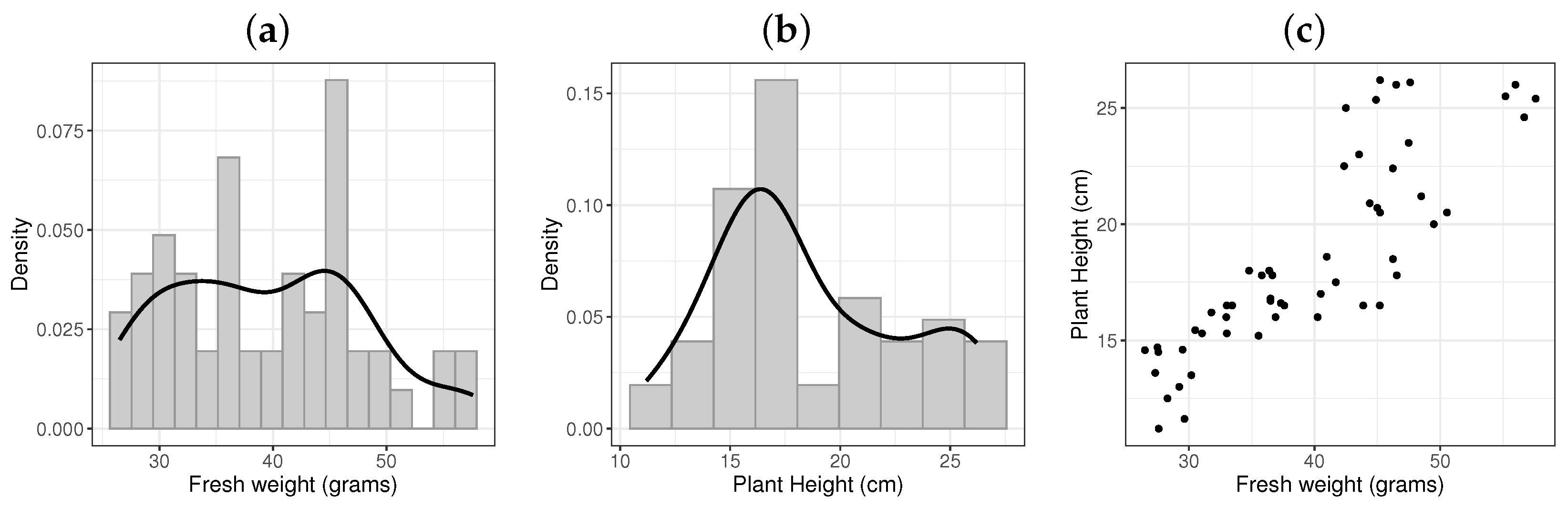
In many practical situations, the response variable presents an asymmetric and/or bimodal behavior. The motivation for this work comes from an experiment carried out at the Plekhanov Russian University of Economics that evaluated the growth of oak leaf lettuce (Lactuca sativa var. crispa). The histograms of the response variables fresh weight (grams) ($y_1$) and plant height (cm) ($y_2$) measured in the experiment are reported in Figure 1a,b. It is noted that they present bimodal behavior and positive asymmetries. In addition, the scatter plot between them (Figure 1c) indicates that they present a strong and positive correlation.

Although a wide range of flexible bivariate distributions can be found in the literature, we note a scarcity of bimodal bivariate distributions. For this purpose, we use the exponentiated odd log-logistic-G (EOLL-G) family (Alizadeh et al., 2020) [19]), whose densities have great flexibility in modeling data, such as bimodality and/or positive or negative asymmetry. The Clayton and Frank copulas are adopted, so the new models are called the BCEOLL-G and BFEOLL-G families, respectively. We consider these copulas because they are suitable to model data with positive correlation (Naifar, 2011) [9] according to the dataset in Figure 1c.

This paper is structured as follows: Section 2 provides a summary of copula functions. Section 3 proposes the bivariate Clayton and Frank copulas generated from the EOLL-G family. Section 4 introduces the Frank and Clayton copulas generated from the EOLL Normal distribution. Section 5 formulates the bivariate bimodal regression with copulas and presents inferential issues. Section 6 performs some simulations for different scenarios. Section 7 illustrates the new methodology for lettuce plants from an experimental trial. Section 8 concludes the article.

2. Archimedean Copulas

According to [20], copulas can be described as functions that link univariate marginal distributions, or alternatively, functions with a multivariate distribution whose marginals are uniform in the interval $[0,1]$. The name and theory of copulas are based on the theorem of Sklar [21]. This important theorem pertaining to the copula method, which guarantees the mentioned relations, is described below. The proof can be found in [22].

Sklar’s Theorem: Let $\mathit{Y}=(Y_1,\dots ,Y_d)$ be a random vector with marginal cumulative distribution functions (cdfs) $F_1\left(y_1\right),\dots ,F_d\left(y_d\right)$, and let $F(y_1\dots ,y_d)$ be their joint cdfs. Define $u_i=F_i\left(y_i\right)=P(Y_i\le y_i),i=1,\dots ,d$. Then, there is a copula function $C(·)$ such that

$$\begin{array}{c}\hfill C(u_1,\dots ,u_d)=P(Y_1\le y_1,\dots ,Y_d\le y_d)=F(y_1,\dots ,y_d).\end{array}$$

(1)

By differentiating (1), the joint probability density function (pdf) follows as

$$\begin{array}{c}\hfill f(y_1,\dots ,y_d)=c(F_1\left(y_1\right),\dots ,F_d\left(y_d\right))\prod _{i=1}^d{f}_i\left(y_i\right),\end{array}$$

(2)

where $f_i\left(y_i\right)$ is the marginal pdf of $Y_i$ and $c(F_1\left(y_1\right),\dots ,F_d\left(y_d\right))$ is the copula density by taking the derivative of the copula function. For independent marginals, $C(u_1,\dots ,u_d)={\prod }_{i=1}^d{u}_i$ and $c(F_1\left(y_1\right),\dots ,F_d\left(y_d\right))=1$, and then $f(y_1,\dots ,y_d)={\prod }_{i=1}^d{f}_i\left(y_i\right)$, which means the independence of the random variables.

Henceforth, we consider the bivariate case for the data introduced in Section 1.

Archimedean copulas are constructed by a strictly decreasing continuous generating function $\phi :[0,1]\to [0,\infty ]$, where $\phi \left(0\right)=\infty$ and $\phi \left(1\right)=0$. Thus, the distribution function of a two-dimensional Archimedean copula can be expressed as

$$C(\mathit{u},\lambda )={\phi }^{-1}(\phi \left(u_1\right)+\phi \left(u_2\right);\lambda ),\mathit{u}={(u_1,u_2)}^{\top },$$

where $\lambda$ is the control parameter of the degree of dependency. The lower and upper tail dependence measures for a bivariate copula C are defined in Joe (1993) [23] (if the limits exist) as

$${\lambda }_{\mathrm{L}}=\underset{u\to 0}{lim}\frac{C(u,u)}{u},{\lambda }_{\mathrm{U}}=\underset{u\to 1}{lim}\frac{1-2u+C(u,u)}{1-u}.$$

For the Archimedean copula, these limits hold

$$\begin{array}{c}\hfill {\lambda }_{\mathrm{L}}=\left\{\begin{array}{cc}\underset{u\to \infty }{lim}{\displaystyle \frac{{\phi }^{-1}\left(2u\right)}{{\phi }^{-1}\left(u\right)}},\hfill & \mathrm{if}\phi \left(0\right)=\infty ,\hfill \\ 0,\hfill & \mathrm{otherwise},\hfill \end{array}\right.{\lambda }_{\mathrm{U}}=2-\underset{u\to 0}{lim}{\displaystyle \frac{1-{\phi }^{-1}\left(2u\right)}{1-{\phi }^{-1}\left(u\right)}}.\end{array}$$

(3)

Here, we employ the most cited bivariate Archimedean copulas (Clayton, 1978 [24]; Frank, 1979 [25]) for constructing new bivariate response regression models.

2.1. Clayton Copula

The Clayton copula [24] has generating function $\phi \left(t\right)=(t^{-\lambda }-1)/\lambda$ and distribution and density functions given by

$$C(u_1,u_2)={(u_1^{-\lambda }+u_2^{-\lambda }-1)}^{-\frac{1}{\lambda }},$$

(4)

and

$$c(u_1,u_2)=(\lambda +1){(u_1^{-\lambda }+u_2^{-\lambda }-1)}^{\frac{-(2\lambda +1)}{\lambda }}{\left(u_1{u}_2\right)}^{-(\lambda +1)},$$

(5)

respectively, where $\lambda >0$. In this case, there is independence between the two variables when $\lambda$ tends to zero. As $\phi \left(0\right)=\infty$ and ${\phi }^{-1}\left(t\right)={(1+\lambda t)}^{-1/\lambda }$, it follows from Equation (3)

$$\begin{array}{c}\hfill {\lambda }_{\mathrm{L}}=\underset{u\to \infty }{lim}{\left(1+\frac{\lambda u}{1+\lambda u}\right)}^{-1/\lambda }=2^{-1/\lambda }\end{array}$$

and

$$\begin{array}{c}\hfill {\lambda }_{\mathrm{U}}=2-\underset{u\to 0}{lim}{\displaystyle \frac{1-{(1+2\lambda u)}^{-1/\lambda }}{1-{(1+\lambda u)}^{-1/\lambda }}}=0.\end{array}$$

2.2. Frank Copula

The Frank copula [25] has generating function $\phi \left(t\right)=-log[(e^{-\lambda t}-1)/(e^{-\lambda }-1)]$ and distribution and density functions given by

$$C(u_1,u_2)=-\frac{1}{\lambda }log\left\{1+\frac{(e^{-\lambda u_1}-1)(e^{-\lambda u_2}-1)}{e^{-\lambda }-1}\right\}$$

(6)

and

$$c(u_1,u_2)=\frac{\lambda e^{-\lambda u_1-\lambda u_2}(1-e^{-\lambda })}{{(e^{-\lambda }-e^{-\lambda u_1}-e^{-\lambda u_2}+e^{-\lambda u_1-\lambda u_2})}^2},$$

(7)

respectively, where $\lambda \in \mathbb{R}\setminus \left\{0\right\}$. If $\lambda$ tends to zero, the two variables can be independent, and if $\lambda$ tends to infinity the two variables are correlated. As $\phi \left(0\right)=-\infty$ and ${\phi }^{-1}\left(t\right)=-log\{1+exp(-t)[exp(-\lambda )-1]\}/\lambda$, it follows from Equation (3) using L’Hôpital rule ${\lambda }_{\mathrm{L}}=0$ and

$$\begin{array}{c}\hfill {\lambda }_{\mathrm{U}}=2-\underset{u\to 0}{lim}{\displaystyle \frac{\lambda +log\{1+{\mathrm{e}}^{-2u}[{\mathrm{e}}^{-\lambda }-1]\}}{\lambda +log\{1+{\mathrm{e}}^{-u}[{\mathrm{e}}^{-\lambda }-1]\}}}=0.\end{array}$$

3. A Bivariate EOLL-G Family Based on Clayton and Frank Copulas

For any baseline cdf $G\left(y\right)=G(y;\mathit{\eta })$ depending on a parameter vector $\mathit{\eta }$, Alizadeh et al. (2020) [19] defined the cdf of the exponentiated odd log-logistic (“EOLL-G”) family (for $y\in \mathbb{R}$) by

$$\begin{array}{c}\hfill F\left(y\right)=F(y;\nu ,\tau ,\mathit{\eta })=\frac{G^{\nu \tau }\left(y\right)}{{\left\{G^{\nu }\left(y\right)+{\left[\overline{G}\left(y\right)\right]}^{\nu }\right\}}^{\tau }},\end{array}$$

(8)

where $\overline{G}\left(y\right)=1-G\left(y\right)$, $\nu >0$ and $\tau >0$ are two extra shape parameters.

The pdf associated to Equation (8) becomes

$$f\left(y\right)=f(y;\nu ,\tau ,\mathit{\eta })=\frac{\nu \tau G^{\nu \tau -1}\left(y\right){\left[\overline{G}\left(y\right)\right]}^{\nu -1}g\left(y\right)}{{\left\{G^{\nu }\left(y\right)+{\left[\overline{G}\left(y\right)\right]}^{\nu }\right\}}^{\tau +1}},$$

(9)

where $g\left(y\right)=dG\left(y\right)/dy$.

From now on, let $Y\sim EOLL-G(\nu ,\tau ,\mathit{\eta })$ be a random variable with pdf (9). Let X have cdf $G(·;\mathit{\eta })$ such that $\mathbb{E}\left(X^p\right)=\int x^{p}g\left(x\right)dx$ (for $p>0$) are finite. Some properties of Y are reported below:

(a)

The positive moments of Y, i.e., $\mathbb{E}\left(Y^p\right)=\int y^{p}f\left(y\right)dy$, $p>0$, are finite when $\nu >1$ (see Appendix A.1).

(b)

The variable Y admits the stochastic representation: $Y=G^{-1}\left(S/(S+1)\right)$, where S has the Dagum distribution with shape parameters $\nu$ and $\tau$, and unit scale, and $G^{-1}(·)$ denotes the inverse function of $G(·)$ (see Appendix A.2).

(c)

The positive moments of the standardization version of Y, say $[Y-\mathbb{E}\left(Y\right)]/\sqrt{\mathrm{Var}\left(Y\right)}$, are finite if $\nu >1$ (see Appendix A.3).

Definition 1. 

Let $Y_1^{\prime },\dots ,Y_d^{\prime }$ be an independent copy of $Y_1,\dots ,Y_d$, i.e., ${\mathit{Y}}^{\prime }=(Y_1^{\prime },\dots ,Y_d^{\prime })$ is independent of $\mathit{Y}=(Y_1,\dots ,Y_d)$ and both have the same joint cdf $F=F_{\mathit{Y}}$. Following Koshevoy (1997) [26], the distance-Gini mean difference for F is

$$\begin{array}{c}\hfill M_D\left(F\right)\equiv \frac{1}{2d}\mathbb{E}(\parallel \mathit{Y}-{\mathit{Y}}^{\prime }\parallel )=\frac{1}{2d}{\int }_{{(0,\infty )}^d}{\int }_{{(0,\infty )}^d}\parallel \mathit{y}-{\mathit{y}}^{\prime }\parallel dF\left(\mathit{y}\right)dF\left({\mathit{y}}^{\prime }\right),\end{array}$$

(10)

where $\parallel ·\parallel$ denotes the Euclidean distance in ${\mathbb{R}}^2$.

(d)

The distance-Gini mean difference $M_D\left(F\right)$ corresponding to the joint cdf F in (1), where $Y_i\sim EOLL-G({\nu }_i,{\tau }_i,{\mathit{\eta }}_i)$, $i=1,\dots ,d$, is finite when $\nu >1$ and X have moments of order greater than one (see Appendix A.4).

(e)

If $U\sim U(0,1)$, then

$$\begin{array}{c}\hfill Q_G\left\{\frac{U^{1/\left(\nu \tau \right)}}{U^{1/\left(\nu \tau \right)}+{(1-U^{1/\tau })}^{1/\nu }}\right\}\sim EOLL-G(\nu ,\tau ,\mathit{\eta }),\end{array}$$

(11)

where $Q_G\left(u\right)=G^{-1}\left(u\right)$ is the quantile function (qf) of G.

The EOLL-G family includes as special cases: the OLL-G class for $\tau =1$ (Gleaton and Lynch, 2006 [27]), and the exponentiated (Exp-G) class (Mudholkar et al., 1996 [28]) for $\nu =1$. Clearly, Equation (9) becomes the baseline G when $\nu =\tau =1$.

Thus, we consider the following marginal distributions

$$\begin{array}{c}\hfill Y_1\sim EOLL-G({\nu }_1,{\tau }_1,{\mathit{\eta }}_1)\mathrm{and}{Y}_2\sim EOLL-G({\nu }_2,{\tau }_2,{\mathit{\eta }}_2),\end{array}$$

(12)

where ${\mathit{\eta }}_1$ and ${\mathit{\eta }}_2$ are parameter vectors of the baseline G, and ${\nu }_1$, ${\tau }_1$, ${\nu }_2$ and ${\tau }_2$ are positive shape parameters.

3.1. BCEOLL-G Model

By inserting (8) and (9) in Equations (1), (2), (4) and (5), the bivariate joint BCEOLL-G cdf reduces to

$$\begin{array}{c}\hfill F_{\mathrm{BCEOLL}-\mathrm{G}}(y_1,y_2)={\left[W_1^{-\lambda }(y_1;{\mathit{\eta }}_1)+W_2^{-\lambda }(y_2;{\mathit{\eta }}_2)-1\right]}^{-\frac{1}{\lambda }}.\end{array}$$

(13)

The corresponding joint pdf has the form

$$\begin{array}{ccc}\hfill f_{\mathrm{BCEOLL}-\mathrm{G}}(y_1,y_2)& =& (\lambda +1){\left[W_1^{-\lambda }(y_1;{\mathit{\eta }}_1)+W_2^{-\lambda }(y_2;{\mathit{\eta }}_2)-1\right]}^{\frac{-(2\lambda +1)}{\lambda }}\times \hfill \\ & & {\left[W_1(y_1;{\mathit{\eta }}_1)W_2(y_2;{\mathit{\eta }}_2)\right]}^{-(\lambda +1)}\times \hfill \\ & & \left[\frac{{\nu }_1{\tau }_1{g}_1(y_1;{\mathit{\eta }}_1)G_1^{{\nu }_1{\tau }_1-1}(y_1;{\mathit{\eta }}_1){\overline{G}}_1^{{\nu }_1-1}(y_1;{\mathit{\eta }}_1)}{H_1^{{\tau }_1+1}(y_1;{\mathit{\eta }}_1)}\right]\times \hfill \\ & & \left[\frac{{\nu }_2{\tau }_2{g}_2(y_2;{\mathit{\eta }}_2)G_2^{{\nu }_2{\tau }_2-1}(y_2;{\mathit{\eta }}_2){\overline{G}}_2^{{\nu }_2-1}(y_2;{\mathit{\eta }}_2)}{H_2^{{\tau }_2+1}(y_2;{\mathit{\eta }}_2)}\right],\hfill \end{array}$$

(14)

where (for $k=1,2$)

$$\begin{array}{c}\hfill H_k(y_k;{\mathit{\eta }}_k)=G_k^{{\nu }_k}(y_k;{\mathit{\eta }}_k)+{[1-G_k(y_k;{\mathit{\eta }}_k)]}^{{\nu }_k},W_k(y_k;{\mathit{\eta }}_k)=\frac{G_k^{{\nu }_k{\tau }_k}(y_k,{\mathit{\eta }}_k)}{H_k^{{\tau }_k}(y_k;{\mathit{\eta }}_k)}.\end{array}$$

3.2. BFEOLL-G Model

Similarly, the joint cdf of the bivariate BFEOLL-G model can be expressed as

$$\begin{array}{cc}\hfill F_{\mathrm{BFEOLL}-\mathrm{G}}(y_1,y_2)& =-\frac{1}{\lambda }log\left\{1+\frac{\left\{exp[-\lambda W_1(y_1;{\mathit{\eta }}_1)]-1\right\}\left\{exp[-\lambda W_2(y_2;{\mathit{\eta }}_2)]-1\right\}}{exp(-\lambda )-1}\right\}.\hfill \end{array}$$

(15)

The corresponding joint BFEOLL-G pdf becomes

$$\begin{array}{cc}\hfill f_{\mathrm{BFEOLL}-\mathrm{G}}(y_1,y_2)& =\lambda [1-exp(-\lambda )]exp\left\{-\lambda \left[W_1(y_1;{\mathit{\eta }}_1)+W_2(y_2;{\mathit{\eta }}_2)\right]\right\}\times \hfill \\ \hfill & {\left\{exp(-\lambda )-exp[-\lambda W_1(y_1;{\mathit{\eta }}_1)]-exp[-\lambda W_2(y_2;{\mathit{\eta }}_2)]+exp[-\lambda (W_1(y_1;{\mathit{\eta }}_1)+W_2(y_2;{\mathit{\eta }}_2))]\right\}}^{-2}\times \hfill \\ \hfill & \left[\frac{{\nu }_1{\tau }_1{g}_1(y_1;{\mathit{\eta }}_1)G_1^{{\nu }_1{\tau }_1-1}(y_1;{\mathit{\eta }}_1){\overline{G}}_1^{{\nu }_1-1}(y_1;{\mathit{\eta }}_1)}{H_1^{{\tau }_1+1}(y_1;{\mathit{\eta }}_1)}\right]\times \hfill \\ \hfill & \left[\frac{{\nu }_2{\tau }_2{g}_2(y_2;{\mathit{\eta }}_2)G_2^{{\nu }_2{\tau }_2-1}(y_2;{\mathit{\eta }}_2){\overline{G}}_2^{{\nu }_2-1}(y_2;{\mathit{\eta }}_2)}{H_2^{{\tau }_2+1}(y_2;{\mathit{\eta }}_2)}\right].\hfill \end{array}$$

(16)

The BCEOLL-G and BFEOLL-G models include three special cases:

• The bivariate Clayton Exponentiated (Exp)-G and Frank Exp-G classes when $\nu =1$;
• The bivariate Clayton odd log-logistic (OLL)-G and Frank OLL-G classes when $\tau =1$.
• The bivariate Clayton and Frank baseline models when $\nu =\tau =1$.

We can generate many bivariate models from Equations (14) and (16) by choosing different parent distributions.

3.3. Copula Dependence Measures

Pearson correlation is one of the most widely used measures, but  it cannot be used in cases where the joint distributions are not normally distributed, and also cannot capture nonlinear relations between the variables.

We study the association of the variables by means of copulas using nonparametric concordance measures for the ranks of the variables, thus enabling coping with data not normally distributed and allowing nonlinear relations between the variables. A concordance measure can be defined as follows: let $(y_{11},y_{21})$ and $(y_{12},y_{22})$ be two observations of the bivariate random variable $(Y_1,Y_2)$. Concordance exists when $(y_{11}-y_{21})(y_{12}-y_{22})>0$, while discordance exists when $(y_{11}-y_{21})(y_{12}-y_{22})<0$.

The Kendall (${\tau }_k$) and Spearman (${\rho }_s$) correlations are concordance measures adopted in this methodology and their expressions derived from the copula dependence parameters are given below:

• Clayton copula: ${\tau }_k=\frac{\lambda }{\lambda +2}$. The expression for ${\rho }_s$ is very complicated.
• Frank copula: ${\tau }_k=1+\frac{4}{\lambda }[D_1\left(\lambda \right)-1]$ and ${\rho }_s=1+\frac{12}{\lambda }[D_2\left(\lambda \right)-D_1\left(\lambda \right)]$, where $D_k(·)$ is the kth order Debye function $\frac{k}{{\alpha }^k}{\int }_0^{\alpha }\frac{t^k}{{\mathrm{e}}^{\mathrm{t}}-1}dt$ (for $k=1,2$).

4. BCEOLL Normal and BFEOLL Normal Models

Here, we discuss special cases of the BCEOLL-G and BFEOLL-G models. The density functions (14) and (16) will be most tractable when the cdf $G_k(y_k;{\mathit{\eta }}_k)$ has a simple analytic expression.

It is known that the data of many experiments follow a normal distribution. So, we present special models considering the normal baseline ($y_k\in \mathbb{R}$)

$$\begin{array}{c}\hfill G_k(y_k;{\mathit{\eta }}_k)=\mathrm{\Phi }\left(\frac{y_k-{\mu }_k}{{\sigma }_k}\right)\mathrm{and}{g}_k(y_k;{\mathit{\eta }}_k)=\frac{1}{{\sigma }_k}\varphi \left(\frac{y_k-{\mu }_k}{{\sigma }_k}\right),\end{array}$$

(17)

where $\mathrm{\Phi }(·)$ and $\varphi (·)$ are the cdf and pdf of the standard normal, respectively, ${\mathit{\eta }}_k={({\mu }_k,{\sigma }_k)}^{\top }$, ${\mu }_k\in \mathbb{R}$ is a location and ${\sigma }_k>0$ is a scale (for $k=1,2$). Hereafter, let $Y_k\sim \mathrm{EOLLN}({\nu }_k,{\tau }_k,{\mu }_k,{\sigma }_k)$ be a random variable.

If the marginals follow the EOLLN distribution, the joint cdf is determined by inserting (17) in Equations (14) and (16). So, the joint pdfs of the BCEOLL Normal (BCEOLLN) and BFEOLL Normal (BFEOLLN) models are

$$\begin{array}{ccc}\hfill f_{\mathrm{BCEOLLN}}(y_1,y_2)& =& (\lambda +1){\left\{{\left[\frac{{\mathrm{\Phi }}^{{\nu }_1{\tau }_1}\left(z_1\right)}{H^{{\tau }_1}\left(z_1\right)}\right]}^{-\lambda }+{\left[\frac{{\mathrm{\Phi }}^{{\nu }_2{\tau }_2}\left(z_2\right)}{H^{{\tau }_2}\left(z_2\right)}\right]}^{-\lambda }-1\right\}}^{-\frac{(2\lambda +1)}{\lambda }}{\left[\frac{{\mathrm{\Phi }}^{{\nu }_1{\tau }_1}\left(z_1\right)}{H^{{\tau }_1}\left(z_1\right)}\times \frac{{\mathrm{\Phi }}^{{\nu }_2{\tau }_2}\left(z_2\right)}{H^{{\tau }_2}\left(z_2\right)}\right]}^{-(\lambda +1)}\times \hfill \\ & & \left\{\frac{{\nu }_1{\tau }_1\varphi \left(z_1\right){\mathrm{\Phi }}^{{\nu }_1{\tau }_1-1}\left(z_1\right){[1-\mathrm{\Phi }\left(z_1\right)]}^{{\nu }_1-1}}{{\sigma }_1{H}^{{\tau }_1}\left(z_1\right)}\right\}\left\{\frac{{\nu }_2{\tau }_2\varphi \left(z_2\right){\mathrm{\Phi }}^{{\nu }_2{\tau }_2-1}\left(z_2\right){[1-\mathrm{\Phi }\left(z_2\right)]}^{{\nu }_2-1}}{{\sigma }_2{H}^{{\tau }_2}\left(z_2\right)}\right\}\hfill \end{array}$$

(18)

and

$$\begin{array}{cc}\hfill f_{\mathrm{BFEOLLN}}(y_1,y_2)& =\lambda [1-exp(-\lambda )]exp\left\{-\lambda \left[\frac{{\mathrm{\Phi }}^{{\nu }_1{\tau }_1}\left(z_1\right)}{H^{{\tau }_1}\left(z_1\right)}+\frac{{\mathrm{\Phi }}^{{\nu }_2{\tau }_2}\left(z_2\right)}{H^{{\tau }_2}\left(z_2\right)}\right]\right\}\times \hfill \\ \hfill & \left\{exp(-\lambda )-exp\left[\frac{-\lambda {\mathrm{\Phi }}^{{\nu }_1{\tau }_1}\left(z_1\right)}{H^{{\tau }_1}\left(z_1\right)}\right]-exp\left[\frac{-\lambda {\mathrm{\Phi }}^{{\nu }_2{\tau }_2}\left(z_2\right)}{H^{{\tau }_2}\left(z_2\right)}\right]+\right.\hfill \\ \hfill & {\left.exp\left[-\lambda \left(\frac{{\mathrm{\Phi }}^{{\nu }_1{\tau }_1}\left(z_1\right)}{H^{{\tau }_1}\left(z_1\right)}+\frac{{\mathrm{\Phi }}^{{\nu }_2{\tau }_2}\left(z_2\right)}{H^{{\tau }_2}\left(z_2\right)}\right)\right]\right\}}^{-2}\times \hfill \\ \hfill & \left\{\frac{{\nu }_1{\tau }_1\varphi \left(z_1\right){\mathrm{\Phi }}^{{\nu }_1{\tau }_1-1}\left(z_1\right){[1-\mathrm{\Phi }\left(z_1\right)]}^{{\nu }_1-1}}{{\sigma }_1{H}^{{\tau }_1}\left(z_1\right)}\right\}\left\{\frac{{\nu }_2{\tau }_2\varphi \left(z_2\right){\mathrm{\Phi }}^{{\nu }_2{\tau }_2-1}\left(z_2\right){[1-\mathrm{\Phi }\left(z_2\right)]}^{{\nu }_2-1}}{{\sigma }_2{H}^{{\tau }_2}\left(z_2\right)}\right\},\hfill \end{array}$$

respectively, where (for $k=1,2$)

$$\begin{array}{c}\hfill \mathrm{\Phi }\left(z_k\right)=\mathrm{\Phi }\left(\frac{y_k-{\mu }_k}{{\sigma }_k}\right),\varphi \left(z_k\right)=\varphi \left(\frac{y_k-{\mu }_k}{{\sigma }_k}\right)\mathrm{and}H\left(z_k\right)={\mathrm{\Phi }}^{{\nu }_k}\left(z_k\right)+{[1-\mathrm{\Phi }\left(z_k\right)]}^{{\nu }_k}.\end{array}$$

(19)

Figure 2 and Figure 3 report the joint densities, their contour plots, and  bivariate cdfs for the Clayton and Frank copulas. The presence of bimodality is noted by the joint density. In the contour plots, we clearly find different association structures.

5. Bivariate Regression Models

Let $(Y_{11},Y_{12}),\cdots ,(Y_{n1},Y_{n2})$ be a bivariate random sample from the BCEOLLN and BEOLLN models, $Y_{ik}\sim \mathrm{BCEOLLN}\left({\mathit{\theta }}_{i1}\right)$ and $Y_{ik}\sim \mathrm{BEOLLN}\left({\mathit{\theta }}_{i2}\right)$, where ${\mathit{\theta }}_{i1}={({\mu }_{i1},{\sigma }_1,{\nu }_1,{\tau }_1)}^{\top }$ and ${\mathit{\theta }}_{i2}={({\mu }_{i2},{\sigma }_2,{\nu }_2,{\tau }_2)}^{\top }$ (for $i=1,\dots ,n$ and $k=1,2$).

Considering a sample $(y_{1k},{\mathit{x}}_{1k}),\cdots ,(y_{nk},{\mathit{x}}_{nk})$, a  systematic component can be defined as

$$\begin{array}{c}\hfill {\mu }_{ik}={\mathbf{x}}_{ik}^{\top }{\mathit{\beta }}_k,\end{array}$$

(20)

where ${\mathbf{x}}_{ik}^{\top }=(1,x_{i1k},\cdots ,x_{ipk})$ is the explanatory variable vector of dimension $p+1$ (for $k=1,2$ and $i=1,\dots ,n$), and ${\mathit{\beta }}_k={({\beta }_{0k},{\beta }_{1k},\cdots ,{\beta }_{pk})}^{\top }$ is the vector of unknown parameters.

Considering n independent observations $(y_{1k},{\mathit{x}}_{1k}),\cdots ,(y_{nk},{\mathit{x}}_{nk})$ (for $k=1,2$), the model defined by (20) and the joint pdf given in Equations (18) and (19). Further, let $z_{ik}=(y_{ik}-{\mu }_{ik})/{\sigma }_k$, $H\left(z_{ik}\right)={\mathrm{\Phi }}^{{\nu }_k}\left(z_{ik}\right)+{[1-\mathrm{\Phi }\left(z_{ik}\right)]}^{{\nu }_k}$, and $W\left(z_{ik}\right)={\mathrm{\Phi }}^{{\nu }_k{\tau }_k}\left(z_{ik}\right)/H^{{\nu }_k}\left(z_{ik}\right)$.

If $\mathit{\theta }={(\lambda ,{\mathit{\theta }}_1^{\top },{\mathit{\theta }}_2^{\top })}^{\top }$, ${\mathit{\theta }}_k={({\mathit{\beta }}_k^{\top },{\sigma }_k,{\tau }_k,{\nu }_k)}^{\top }$, ${\mathit{\beta }}_k^{\top }=({\beta }_{0k},{\beta }_{1k},\cdots ,{\beta }_{pk})$ (for $k=1,2$), the total log-likelihood functions for $\mathit{\theta }$ have the forms below:

BCEOLLN regression model

$$\begin{array}{ccc}\hfill l\left(\mathit{\theta }\right)& =& nlog\left[\frac{(\lambda +1){\nu }_1{\tau }_1{\nu }_2{\tau }_2}{{\sigma }_1{\sigma }_2}\right]-\frac{2\lambda +1}{\lambda }\sum _{i=1}^{n}log\left[W^{-\lambda }\left(z_{i1}\right)+W^{-\lambda }\left(z_{i2}\right)-1\right]-\hfill \\ & & (\lambda +1)\sum _{i=1}^{n}log\left[W\left(z_{i1}\right)W\left(z_{i2}\right)\right]+\sum _{i=1}^{n}log\left\{\frac{\varphi \left(z_{i1}\right){\mathrm{\Phi }}^{{\nu }_1{\tau }_1-1}\left(z_{i1}\right){[1-\mathrm{\Phi }\left(z_{i1}\right)]}^{\nu -1}}{H^{{\tau }_1}\left(z_{i1}\right)}\right\}+\hfill \\ & & \sum _{i=1}^{n}log\left\{\frac{\varphi \left(z_{i2}\right){\mathrm{\Phi }}^{{\nu }_1{\tau }_2-1}\left(z_{i2}\right){[1-\mathrm{\Phi }\left(z_{i2}\right)]}^{\nu -1}}{H^{{\tau }_2}\left(z_{i2}\right)}\right\}.\hfill \end{array}$$

(21)

BFEOLLN regression model

$$\begin{array}{ccc}\hfill l\left(\mathit{\theta }\right)& =& nlog\left\{\frac{\lambda [1-exp(-\lambda )]{\nu }_1{\tau }_1{\nu }_2{\tau }_2}{{\sigma }_1{\sigma }_2}\right\}-\lambda \sum _{i=1}^n[W\left(z_{i1}\right)+W\left(z_{i2}\right)]-\hfill \\ & & 2\sum _{i=1}^{n}log\left\{exp(-\lambda )-exp[-\lambda W\left(z_{i1}\right)]-exp[-\lambda W\left(z_{i2}\right)]+exp[-\lambda (W\left(z_{i1}\right)+W\left(z_{i2}\right))]\right\}+\hfill \\ & & \sum _{i=1}^{n}log\left\{\frac{\varphi \left(z_{i1}\right){\mathrm{\Phi }}^{{\nu }_1{\tau }_1-1}\left(z_{i1}\right){[1-\mathrm{\Phi }\left(z_{i1}\right)]}^{\nu -1}}{H^{{\tau }_1}\left(z_{i1}\right)}\right\}+\hfill \\ & & \sum _{i=1}^{n}log\left\{\frac{\varphi \left(z_{i2}\right){\mathrm{\Phi }}^{{\nu }_1{\tau }_2-1}\left(z_{i2}\right){[1-\mathrm{\Phi }\left(z_{i2}\right)]}^{\nu -1}}{H^{{\tau }_2}\left(z_{i2}\right)}\right\}.\hfill \end{array}$$

(22)

For copulas, the estimation of the parameters is usually conducted in two stages to create bivariate response models. In the first stage, the events are considered independent and the parameters are estimated marginally. The estimates are then used in the second stage, where the association parameter $\alpha$ is estimated. This approach is coherent when the focus of the study is to estimate the association parameter $\lambda$. If the coefficients of the regression are the focus, this marginal two-stage approach does not add any additional information compared to the use of independent models. Then, it is best to conduct a joint estimation of the regression coefficients and $\lambda$.

The maximum likelihood estimate (MLE) $\widehat{\mathit{\theta }}$ can be calculated by maximizing (21) and (22). We use the simplex method of Nelder and Mead (1965) [29] implemented in the optim function in the R software [30]. This method is a robust and direct search method, which uses only function values, i.e., it does not use gradient information. It compares the function values at the vertices of a general simplex, then replaces the vertex with the highest value by another point. The simplex adapts itself to the local landscape, and contracts on to the final minimum. Initial values for $\mathit{\beta }$, ${\sigma }_1$ and ${\sigma }_2$ are taken from the fits of the sub-models with ${\tau }_1={\nu }_1=0.5$ and ${\tau }_2={\nu }_2=0.5$. It proves to be effective, computationally compact and provides the Hessian matrix, necessary for inference. See [29] for details. The asymptotic normal distribution of $\widehat{\mathit{\theta }}$ can be considered for inference, tests, and confidence intervals.

6. Simulation Study

A Monte Carlo simulation study examines the accuracy of the estimates in the bivariate EOLLN regression model. We use the Multivariate Copula Description (MvCD) from the copula package [31] in R. The MvCD function generates the required univariate marginals according to the supplied association parameter using the inverse transformation method.

We consider the sample sizes $n=50,100,200,500$, $r=1000$ replications and a covariate $x_1\sim \mathrm{Normal}(1,0.5)$ related to $y_1$ and $y_2$ by the identity link functions ${\mu }_{i1}=({\beta }_{101}+{\beta }_{111}{x}_{i1})$ and ${\mu }_{i2}=({\beta }_{102}+{\beta }_{112}{x}_{i1})$, respectively. Further, we take ${\sigma }_k=exp\left({\beta }_{20k}\right)$, ${\nu }_k=exp\left({\beta }_{30k}\right)$ and ${\tau }_k=exp\left({\beta }_{40k}\right)$. Then, let $Y_k\sim \mathrm{EOLLN}({\mu }_{ik},{\sigma }_k,{\nu }_k,{\tau }_k)$ (for $k=1,2$), the quantile function (qf) has the form

$$\begin{array}{c}\hfill y_k=Q\left(u\right)=Q_N\left\{\frac{u^{1/\left({\nu }_k{\tau }_k\right)}}{u^{1/\left({\nu }_k{\tau }_k\right)}+{(1-u^{1/{\tau }_k})}^{1/{\nu }_k}}\right\},0<u<1,\end{array}$$

(23)

where $Q_N\left(p\right)={\mathrm{\Phi }}^{-1}(p;{\mu }_k,{\sigma }_k)$, $p\in (0,1)$, is the normal qf, namely

$$\begin{array}{c}\hfill {\mathrm{\Phi }}^{-1}(p;{\mu }_k,{\sigma }_k)={\mu }_k+\sqrt{2}{\sigma }_k{\mathrm{erf}}^{-1}(2p-1)\end{array}$$

(24)

and ${\mathrm{erf}}^{-1}(·)$ is the inverse error function.

The true parameter values are: ${\mu }_{i1}=(1.5+1.32x_{i1}),{\sigma }_1=exp\left(1.5\right),{\nu }_1=exp\left(1.1\right),{\tau }_1=exp\left(1.4\right),{\mu }_{i2}=(1.6+2.3x_{i1}),{\sigma }_2=exp\left(0.6\right)$, ${\nu }_2=exp\left(1.8\right),{\tau }_2=exp\left(1.9\right)$ and $\lambda =5$.

The average estimates (AEs), biases, and mean squared errors (MSEs) are given by

$$\mathrm{AE}\left(\widehat{\eta }\right)=\frac{1}{r}\sum _{i=1}^r\widehat{{\eta }_i},\mathrm{Bias}\left(\widehat{\eta }\right)=\frac{1}{r}\sum _{i=1}^r(\widehat{{\eta }_i}-{\eta }_i),\mathrm{MSE}\left(\widehat{\eta }\right)=\frac{1}{r}\sum _{i=1}^r{(\widehat{{\eta }_i}-{\eta }_i)}^2,$$

(25)

where ${\widehat{\eta }}^{\top }=({\widehat{\beta }}_{101},{\widehat{\beta }}_{111},{\widehat{\beta }}_{201},{\widehat{\beta }}_{301},{\widehat{\beta }}_{401},{\widehat{\beta }}_{102},{\widehat{\beta }}_{112},{\widehat{\beta }}_{202},{\widehat{\beta }}_{302},{\widehat{\beta }}_{402},\widehat{\lambda })$.

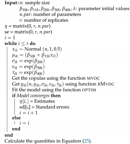
For each of the Clayton and Frank copulas and sample size, the calculations follow the Algorithm 1.

Algorithm 1:

For both copulas, the biases and MSEs in

Table 1. Simulation findings from the fitted bivariate Clayton EOLLN regression model.

$\mathit{\eta }$	True Value		$\mathit{n}=50$			$\mathit{n}=100$
		AEs	Biases	MSEs	AEs	Biases	MSEs
${\beta }_{101}$	1.50	1.4840	−0.0160	0.1436	1.4949	−0.0051	0.0787
${\beta }_{111}$	1.32	1.3206	0.0006	0.0523	1.3190	−0.0010	0.0244
${\beta }_{201}$	1.50	1.5448	0.0448	0.0755	1.5383	0.0383	0.0405
${\beta }_{301}$	1.10	1.1799	0.0799	0.0816	1.1577	0.0577	0.0450
${\beta }_{401}$	1.40	1.4555	0.0555	0.0892	1.4233	0.0233	0.0453
${\beta }_{102}$	1.60	1.5966	−0.0034	0.0056	1.5986	−0.0014	0.0024
${\beta }_{112}$	2.30	2.3003	0.0003	0.0017	2.2991	−0.0009	0.0008
${\beta }_{202}$	0.60	0.6135	0.0135	0.0484	0.6132	0.0132	0.0224
${\beta }_{302}$	1.80	1.8481	0.0481	0.0487	1.8314	0.0314	0.0216
${\beta }_{402}$	1.90	1.9731	0.0731	0.0956	1.9396	0.0396	0.0408
$\lambda$	5.00	5.2268	0.2268	0.1417	5.1446	0.1446	0.0601
$\mathit{\eta }$	True Value		$\mathit{n}=200$			$\mathit{n}=500$
		AEs	Biases	MSEs	AEs	Biases	MSEs
${\beta }_{101}$	1.50	1.4949	−0.0051	0.0437	1.5049	0.0049	0.0164
${\beta }_{111}$	1.32	1.3172	−0.0028	0.0122	1.3219	0.0019	0.0049
${\beta }_{201}$	1.50	1.5336	0.0336	0.0247	1.5185	0.0185	0.0108
${\beta }_{301}$	1.10	1.1440	0.0440	0.0272	1.1253	0.0253	0.0112
${\beta }_{401}$	1.40	1.4147	0.0147	0.0214	1.3992	−0.0008	0.0074
${\beta }_{102}$	1.60	1.5985	−0.0015	0.0010	1.5993	−0.0007	0.0003
${\beta }_{112}$	2.30	2.2996	−0.0004	0.0004	2.3003	0.0003	0.0002
${\beta }_{202}$	0.60	0.6149	0.0149	0.0100	0.6089	0.0089	0.0048
${\beta }_{302}$	1.80	1.8244	0.0244	0.0093	1.8135	0.0135	0.0045
${\beta }_{402}$	1.90	1.9215	0.0215	0.0174	1.9078	0.0078	0.0057
$\lambda$	5.00	5.0736	0.0736	0.0223	5.0178	0.0178	0.0060

and

Table 2. Simulation findings from the fitted bivariate Frank EOLLN regression model.

$\mathit{\eta }$	True Value		$\mathit{n}=50$			$\mathit{n}=100$
		AEs	Biases	MSEs	AEs	Biases	MSEs
${\beta }_{101}$	1.50	1.3278	−0.1722	0.5729	1.3552	−0.1448	0.3244
${\beta }_{111}$	1.32	1.3110	−0.0090	0.0905	1.3250	0.0050	0.0432
${\beta }_{201}$	1.50	1.5802	0.0802	0.0891	1.5753	0.0753	0.0686
${\beta }_{301}$	1.10	1.2140	0.1140	0.1023	1.1875	0.0875	0.0734
${\beta }_{401}$	1.40	1.6102	0.2102	0.4140	1.5419	0.1419	0.2325
${\beta }_{102}$	1.60	1.5604	−0.0396	0.0195	1.5730	−0.0270	0.0114
${\beta }_{112}$	2.30	2.2977	−0.0023	0.0037	2.3015	0.0015	0.0017
${\beta }_{202}$	0.60	0.6307	0.0307	0.0566	0.6419	0.0419	0.0446
${\beta }_{302}$	1.80	1.8510	0.0510	0.0667	1.8546	0.0546	0.0483
${\beta }_{402}$	1.90	2.1430	0.2430	0.3737	2.0495	0.1495	0.2159
$\lambda$	5.00	5.1239	0.1239	0.3300	5.0954	0.0954	0.2026
$\mathit{\eta }$	True Value		$n=200$			$n=500$
		AEs	Biases	MSEs	AEs	Biases	MSEs
${\beta }_{101}$	1.50	1.4714	−0.0286	0.1427	1.4853	−0.0147	0.0666
${\beta }_{111}$	1.32	1.3145	−0.0055	0.0225	1.3264	0.0064	0.0086
${\beta }_{201}$	1.50	1.5681	0.0681	0.0390	1.5407	0.0407	0.0189
${\beta }_{301}$	1.10	1.1789	0.0789	0.0414	1.1461	0.0461	0.0210
${\beta }_{401}$	1.40	1.4391	0.0391	0.0999	1.4102	0.0102	0.0421
${\beta }_{102}$	1.60	1.5801	−0.0199	0.0052	1.5862	−0.0138	0.0024
${\beta }_{112}$	2.30	2.2990	−0.0010	0.0008	2.3008	0.0008	0.0003
${\beta }_{202}$	0.60	0.6271	0.0271	0.0217	0.6278	0.0278	0.0100
${\beta }_{302}$	1.80	1.8334	0.0334	0.0225	1.8289	0.0289	0.0094
${\beta }_{402}$	1.90	2.0108	0.1108	0.0961	1.9652	0.0652	0.0465
$\lambda$	5.00	5.0431	0.0431	0.0856	5.0227	0.0227	0.0428

decrease when n grows. So, the consistency of the estimators holds. The empirical coverage probabilities (CPs) in

Table 3. CPs for the fitted bivariate Clayton and Frank EOLLN regression models.

Clayton
n	${\beta }_{101}$	${\beta }_{111}$	${\beta }_{201}$	${\beta }_{301}$	${\beta }_{401}$	${\beta }_{102}$	${\beta }_{112}$	${\beta }_{202}$	${\beta }_{302}$	${\beta }_{402}$	$\lambda$
50	0.995	0.971	0.999	0.996	0.997	0.999	0.972	1.000	1.000	0.999	0.961
100	0.996	0.972	0.998	0.997	0.998	1.000	0.974	1.000	1.000	1.000	0.962
200	0.999	0.958	0.999	0.999	1.000	0.999	0.965	1.000	0.999	1.000	0.968
500	0.999	0.962	0.999	0.999	1.000	1.000	0.964	1.000	1.000	1.000	0.948
Frank
n	${\beta }_{101}$	${\beta }_{111}$	${\beta }_{201}$	${\beta }_{301}$	${\beta }_{401}$	${\beta }_{102}$	${\beta }_{112}$	${\beta }_{202}$	${\beta }_{302}$	${\beta }_{402}$	$\lambda$
50	0.983	0.956	1.000	0.998	0.986	0.988	0.937	1.000	1.000	0.988	0.950
100	0.993	0.961	0.999	1.000	0.992	0.989	0.944	1.000	0.999	0.990	0.951
200	0.990	0.956	0.999	0.998	0.991	0.996	0.956	1.000	1.000	0.997	0.962
500	0.995	0.955	0.999	0.999	0.995	0.998	0.946	1.000	1.000	0.997	0.953

show that their values converge to the 95% nominal level.

7. Application to Lettuce Leaf Data

This dataset refers to the effect of the foliar application of different concentrations of silicon dioxide and organosilicon compounds on the growth and biochemical contents of Lactuca sativa var. crispa grown in phytotron conditions. The experiment was carried out on 12 March 2020, in the Department of Goods Commodity and Expertise of Goods Products in Moscow, Russian Federation. More details of the experiment are described in [32]. Here, we check the response variables fresh weight (grams) ($y_1$) and plant height (cm) ($y_2$) together in order to verify the existing correlation between them. We also present a regression model relating these covariates with the following treatments:

The levels of gradual concentrations of amorphous silicon dioxide (AS) and 1-ethoxysilatrane (ES) solutions are: AS1 (50 mg·L${}^{-1}$), AS2 (100 mg·L${}^{-1}$), AS3 (200 mg·L${}^{-1}$), AS4 (300 mg·L${}^{-1}$), and ES1 (5 × 10${}^{-4}$ mL·L${}^{-1}$), ES2 (10${}^{-3}$ mL·L${}^{-1}$), ES3 (5 × 10${}^{-3}$ mL·L${}^{-1}$) and ES4 (10${}^{-2}$ mL·L${}^{-1}$). These variables are defined by dummy variables as follows:

• $y_{i1}$ fresh weight (grams);
• $y_{i2}$ plant height (cm);
• $x_{ijk}$ combination of AS and ES solutions (for $j=1\dots 8$).

Hence, the systematic component has the form (for $k=1,2$ and $i=1,\dots ,54$):

$${\mu }_{ik}={\beta }_{0k}+{\beta }_{1k}{x}_{i1k}+{\beta }_{2k}{x}_{i2k}+{\beta }_{3k}{x}_{i3k}+{\beta }_{4k}{x}_{i4k}+{\beta }_{5k}{x}_{i5k}+{\beta }_{6k}{x}_{i6k}+{\beta }_{7k}{x}_{i7k}+{\beta }_{8k}{x}_{i8k}.$$

7.1. Descriptive Analysis

First, we present a descriptive analysis of the dataset.

Table 4. Descriptive analysis of fresh weight ($y_1$) and plant height ($y_2$) variables.

Variable	Mean	Median	s.d.	Min.	Max	Skewness	VC	Kurtosis
$y_1$	39.511	38.925	8.406	26.500	57.610	0.268	21.274	2.208
$y_2$	18.485	17.250	4.197	11.200	26.200	0.476	22.707	2.174

indicates positive asymmetry and kurtosis for both response variables. Figure 1a,b displays the histograms of these variables, thus indicating bimodal behavior for both. Pearson’s coefficient is $0.8497$, which is a strong positive correlation, as can be noted in Figure 1. Figure 4 provides the boxplots for different experimental treatments.

7.2. Univarite Marginal Analysis

Univariate analysis of the response variables is conducted under the EOLLN distribution and its special cases: OLLN, Exp-N, and Normal. The Akaike information criterion (AIC) and Global Deviance (GD) in

Table 5. Adequacy measures of the univariate models for each response variable.

Model	Fresh Weight		Plant Height
	AIC	GD	AIC	GD
EOLLN	385.98	377.98	300.80	292.80
OLLN	384.05	378.05	305.51	299.51
Exp-N	387.40	381.40	309.57	303.57
Normal	386.16	382.16	311.16	307.16

reveal that the OLLN model is more adequate for $y_1$ (fresh weight) and the EOLLN model for $y_2$ (plant height).

Figure 5a and Figure 6a report the histograms with estimated densities, and Figure 5b and Figure 6b their empirical and estimated cumulative distributions, thus supporting the findings in Table 5.

7.3. Bivariate Analysis and Regression Model

Next, we carry out a joint analysis of the response variables from the current sixteen models for the Clayton and Frank copulas.

Table 6. AIC, GD, copula dependence parameter ($\lambda$), Kendall correlation (${\tau }_k$) and Spearman correlation (${\rho }_s$) for sixteen bivariate models fitted to lettuce data.

Model for (${\mathit{Y}}_1\times {\mathit{Y}}_2$)	Clayton					Frank
	AIC	GD	$\mathit{\lambda }$	${\mathit{\tau }}_{\mathit{k}}$	${\mathit{\rho }}_{\mathit{s}}$	AIC	GD	$\mathit{\lambda }$	${\mathit{\tau }}_{\mathit{k}}$	${\mathit{\rho }}_{\mathit{s}}$
EOLLN × EOLLN	623.18	605.18	2.81	0.58	0.77	615.95	597.95	10.16	0.67	0.86
EOLLN × OLLN	634.02	618.02	2.27	0.53	0.72	627.92	611.92	9.67	0.66	0.85
EOLLN × Exp-N	629.52	613.52	3.38	0.63	0.81	628.37	612.37	8.60	0.62	0.82
EOLLN × Normal	625.02	611.02	3.58	0.64	0.83	630.43	616.43	10.23	0.67	0.87
OLLN × EOLLN	620.25	604.25	2.93	0.59	0.78	612.78	596.78	10.79	0.69	0.88
OLLN × OLLN	632.00	618.00	2.31	0.54	0.72	626.71	612.71	9.47	0.65	0.85
OLLN × Exp-N	628.19	614.19	3.36	0.63	0.81	623.88	609.88	10.25	0.67	0.87
OLLN × Normal	624.47	612.47	3.82	0.66	0.84	628.43	616.43	10.36	0.68	0.87
Exp-N × EOLLN	622.61	606.61	2.92	0.59	0.78	616.98	600.98	10.03	0.67	0.86
Exp-N × OLLN	631.90	617.90	2.87	0.59	0.78	632.15	618.15	9.11	0.64	0.84
Exp-N × Exp-N	632.43	618.43	3.47	0.63	0.82	636.22	622.22	10.85	0.69	0.88
Exp-N × Normal	626.75	614.75	3.33	0.62	0.81	632.04	620.04	9.80	0.66	0.86
Normal × EOLLN	620.62	606.62	3.00	0.60	0.79	615.77	601.77	10.30	0.67	0.87
Normal × OLLN	633.50	621.50	2.29	0.53	0.72	630.58	618.58	9.15	0.64	0.84
Normal × Exp-N	629.29	617.29	3.05	0.60	0.79	624.74	612.74	10.16	0.67	0.86
Normal × Normal	624.54	614.54	3.35	0.63	0.81	630.37	620.37	9.99	0.67	0.86

reveals that the bivariate (OLLN × EOLLN) regression model with Clayton and Frank copulas is the most suitable model to explain the response variables ($Y_1\times Y_2$), thus agreeing with the univariate analysis.

Additionally, we provide the values of the copula dependence parameter ($\lambda$), Kendall’s correlation (${\tau }_k$), and Spearman correlation (${\rho }_s$). For both models and the two copulas, these values indicate that the variables have strong positive dependence, thus confirming the required dependence structure.

Table 7. Estimated quantities for the best bivariate regression model fitted to lettuce data.

$\mathit{\theta }$	MLEs	CIs	SEs	p-Values
${\beta }_{01}$	35.8036	[33.7814, 37.8257]	1.0086	<0.001
${\beta }_{11}$	10.8022	[8.1460, 13.4583]	1.3248	<0.001
${\beta }_{21}$	9.9009	[7.1183, 12.6833]	1.3879	<0.001
${\beta }_{31}$	−7.6892	[−10.3286, −5.0497]	1.3165	<0.001
${\beta }_{41}$	−6.7391	[−9.2985, −4.1795]	1.2766	<0.001
${\beta }_{51}$	0.6059	[−2.1540, 3.3658]	1.3766	0.3308
${\beta }_{61}$	−0.1776	[−3.0838, 2.7287]	1.4496	0.4515
${\beta }_{71}$	8.4060	[5.3443, 11.4675]	1.5271	<0.001
${\beta }_{81}$	18.6657	[15.5123, 21.8191]	1.5729	<0.001
$log\left({\sigma }_1\right)$	1.8421	[−4.0207, 7.7049]	2.9243
$log\left({\nu }_1\right)$	1.0892	[−4.9764, 7.1548]	3.0255
${\beta }_{02}$	17.0122	[15.8189, 18.2056]	0.5952	<0.001
${\beta }_{12}$	9.4337	[8.1786, 10.6887]	0.6259	<0.001
${\beta }_{22}$	1.6790	[0.0778, 3.2802]	0.7986	0.0201
${\beta }_{32}$	−1.6034	[−2.7452, −0.4617]	0.5694	0.0034
${\beta }_{42}$	−3.2964	[−4.6713, −1.9214]	0.6857	<0.001
${\beta }_{52}$	0.9021	[−0.4202, 2.2245]	0.6595	0.0885
${\beta }_{62}$	1.0147	[−0.2440, 2.2736]	0.6279	0.0559
${\beta }_{72}$	6.3580	[4.5401, 8.1759]	0.9067	<0.001
${\beta }_{82}$	8.3849	[7.0828, 9.6870]	0.6494	<0.001
$log\left({\sigma }_2\right)$	0.7811	[−1.6658, 3.2282]	1.2205
$log\left({\nu }_2\right)$	1.1064	[−1.0946, 3.3074]	1.0978
$log\left(\tau \right)$	−1.0721	[−2.6434, 0.4992]	0.7837
$\lambda$	3.3776	[1.1464,5.6086]	1.1129
${\tau }_k$=0.339, ${\rho }_s$= 0.492			AIC: 456.7843 GD: 408.7843

provides the estimated quantities for the best bivariate regression model.

We can conclude the following facts:

• Interpretations for $\mu$:

  -

  Comparison of the treatments with the control indicates that treatments ES1 and ES2 are not significant for the metrics of fresh mass and plant height. The other treatments are significant for both variables.

  -

  Comparison of the treatments with the control indicates that treatments AS1, AS2, ES3, and ES4 have positive effects on the fresh mass. So, they increase with the fresh mass. On the other hand, the effects of treatments AS3 and AS4 are negative for the fresh mass.

  -

  For the plant height, the treatments AS1, AS2, ES3, and ES4 have positive effects, meaning greater height in relation to the control. In contrast, the treatments AS3 and AS4 have negative effects on plant height.

  -

  Table 8. Comparisons between treatments according to the best bivariate regression model.

  Hypotheses ${\mathit{H}}_0$	Fresh Weight			Plant Height
  	MLEs	SEs	p-Values	MLEs	SEs	p-Values
  AS1 - Control	10.802	1.325	0.000	9.434	0.626	0.000
  AS2 - Control	9.901	1.388	0.000	1.679	0.799	0.020
  AS3 - Control	−7.689	1.317	0.000	−1.603	0.569	0.003
  AS4 - Control	−6.739	1.277	0.000	−3.296	0.686	0.000
  ES1 - Control	0.606	1.377	0.331	0.902	0.660	0.088
  ES2 - Control	−0.178	1.450	0.452	1.015	0.628	0.056
  ES3 - Control	8.406	1.527	0.000	6.358	0.907	0.000
  ES4 - Control	18.666	1.573	0.000	8.385	0.649	0.000
  AS1 - ES4	−8.160	2.453	0.001	0.959	0.745	0.102
  AS2 - ES4	−9.017	2.097	0.000	−6.829	0.902	0.000
  AS3 - ES4	−26.352	2.667	0.000	−9.975	0.754	0.000
  AS4 - ES4	−25.410	2.495	0.000	−11.658	0.855	0.000
  ES1 - ES4	−18.376	2.642	0.000	−7.505	0.843	0.000
  ES2 - ES4	−18.741	2.638	0.000	−7.312	0.810	0.000
  ES3 - ES4	−10.192	2.853	0.000	−1.956	1.061	0.035
  AS1 - ES3	2.663	1.581	0.049	3.120	1.159	0.005
  AS2 - ES3	1.935	1.436	0.092	−4.597	0.859	0.000
  AS3 - ES3	−15.784	1.599	0.000	−7.802	1.088	0.000
  AS4 - ES3	−14.686	1.417	0.000	−9.550	0.922	0.000
  ES1 - ES3	−7.468	1.504	0.000	−5.323	0.892	0.000
  ES2 - ES3	−8.035	1.667	0.000	−5.143	1.033	0.000
  AS1 - ES2	10.396	1.446	0.000	8.377	0.678	0.000
  AS2 - ES2	9.707	1.464	0.000	0.689	0.841	0.208
  AS3 - ES2	−7.959	1.399	0.000	−2.592	0.636	0.000
  AS4 - ES2	−6.875	1.367	0.000	−4.295	0.713	0.000
  ES1 - ES2	0.255	1.492	0.432	−0.120	0.701	0.432
  AS1 - ES1	10.414	1.358	0.000	8.562	0.788	0.000
  AS2 - ES1	9.640	1.339	0.000	0.918	0.764	0.117
  AS3 - ES1	−7.931	1.363	0.000	−2.409	0.718	0.001
  AS4 - ES1	−7.025	1.243	0.000	−4.117	0.694	0.000
  AS1 - AS4	17.472	1.218	0.000	12.768	0.794	0.000
  AS2 - AS4	16.701	1.129	0.000	4.995	0.781	0.000
  AS3 - AS4	−1.036	1.191	0.194	1.715	0.715	0.010
  AS1 - AS3	18.338	1.252	0.000	10.951	0.591	0.000
  AS2 - AS3	17.712	1.303	0.000	3.355	0.875	0.000
  AS1 - AS2	1.090	1.315	0.205	7.782	0.977	0.000

  compares all treatments with the corresponding control, from which other interpretations can be found.

  -

  All the results are clearly consistent with the descriptive analysis.

• Interpretations for $\lambda$, ${\tau }_k$ and ${\rho }_s$:

  -

  The values of $\lambda$, ${\tau }_k$, and ${\rho }_s$ in the best regression model reveal that the variables are correlated with moderate dependence. The dependence structure is necessary, as confirmed by the 95% CIs for the dependence parameter of the copula, which does not include zero.

Finally, Figure 7 displays the plots of the observed and predicted values and corresponding CIs, thus supporting that the best bivariate regression model is a good predictor for the current data.

8. Conclusions

This article proposed a new bivariate family based on Archimedean copulas. Motivated by an experiment that evaluated the growth of oak lettuce plants, which presented the variables fresh mass and height with bimodal behavior, we used the exponentiated odd log-logistic family, whose densities can model different types of data, including bimodality. Furthermore, these variables showed a strong positive correlation and the Clayton and Frank copulas were suitable for studying data with a positive correlation.

We presented some mathematical properties of the new family and a simulation study showed the consistency of the maximum likelihood estimators. We considered two categorical explanatory variables (each one with four treatments) to explain two response variables: fresh weight and plant height. Some important results were obtained from the application: (i) For both variables, the same treatments were significant or not; (ii) Two treatments had negative effects on the two variables and two other treatments had the greatest effects on the variables, i.e., with these treatments greater fresh mass and greater plant height were obtained. The bivariate regression model proved to be adequate for predicting fresh weight and plant height values of oak lettuce under the effect of different treatments. The choice of these copulas proved to be adequate due to the positive dependence structure between the variables. Other baseline distributions can be used as well as applications in other areas of knowledge.

References

- Nelsen, R.B. Properties of a one-parameter family of bivariate distributions with specified marginals. Commun. Stat.-Theory Methods 1986, 15, 3277–3285. [Google Scholar] [CrossRef]
- Quiroz-Flores, A. Testing copula functions as a method to derive bivariate Weibull distributions. In Proceedings of the APSA Annual Meeting & Exhibition, Toronto, ON, Canada, 3–6 September 2009. [Google Scholar]
- El-Sherpieny, E.S.; Almetwally, E.M. Bivariate generalized rayleigh distribution based on Clayton Copula. In Proceedings of the 54rd Annual Conference on Statistics, Computer Science and Operation Research, Cairo, Egypt, 9–11 December 2019; pp. 1–19. [Google Scholar]
- Almetwally, E.M.; Muhammed, H.Z. On a Bivariate Frechet Distribution. J. Stat. Appl. Probab. 2020, 9, 1–21. [Google Scholar]
- Muhammed, H.Z. On a bivariate generalized inverted Kumaraswamy distribution. Phys. A Stat. Mech. Its Appl. 2020, 553, 124281. [Google Scholar] [CrossRef]
- Samanthi, R.G.M.; Sepanski, J. On bivariate Kumaraswamy-distorted copulas. Commun. Stat.-Theory Methods 2022, 51, 2477–2495. [Google Scholar] [CrossRef]
- Alotaibi, R.M.; Rezk, H.R.; Ghosh, I.; Dey, S. Bivariate exponentiated half logistic distribution: Properties and application. Commun. Stat.-Theory Methods 2021, 50, 6099–6121. [Google Scholar] [CrossRef]
- Vaidyanathan, V.S.; Sharon Varghese, A. Morgenstern type bivariate Lindley distribution. Stat. Optim. Inf. Comput. 2016, 4, 132–146. [Google Scholar] [CrossRef]
- Naifar, N. Modelling dependence structure with Archimedean copulas and applications to the iTraxx CDS index. J. Comput. Appl. Math. 2011, 235, 2459–2466. [Google Scholar] [CrossRef]
- Yang, L.; Cai, X.J.; Li, M.; Hamori, S. Modeling dependence structures among international stock markets: Evidence from hierarchical Archimedean copulas. Econ. Model. 2015, 51, 308–314. [Google Scholar] [CrossRef]
- Novianti, P.; Kartiko, S.H.; Rosadi, D. Application of Clayton Copula to identify dependency structure of COVID-19 outbreak and average temperature in Jakarta Indonesia. J. Phys. Conf. Ser. 2021, 1, 012154. [Google Scholar] [CrossRef]
- Li, H.; Lu, Y. Modeling cause-of-death mortality using hierarchical Archimedean copula. Scand. Actuar. J. 2019, 3, 247–272. [Google Scholar] [CrossRef]
- Janga Reddy, M.; Ganguli, P. Risk assessment of hydroclimatic variability on groundwater levels in the Manjara basin aquifer in India using Archimedean copulas. J. Hydrol. Eng. 2012, 17, 1345–1357. [Google Scholar] [CrossRef]
- Zhang, L.; Singh, V.P. Bivariate rainfall frequency distributions using Archimedean copulas. J. Hydrol. 2007, 332, 93–109. [Google Scholar] [CrossRef]
- Tsakiris, G.; Kordalis, N.; Tigkas, D.; Tsakiris, V.; Vangelis, H. Analysing drought severity and areal extent by 2D Archimedean copulas. Water Resour. Manag. 2016, 30, 5723–5735. [Google Scholar] [CrossRef]
- He, W.; Lawless, J.F. Bivariate location–scale models for regression analysis, with applications to lifetime data. J. R. Stat. Soc. Ser. B (Stat. Methodol.) 2005, 67, 63–78. [Google Scholar] [CrossRef]
- Wienke, A.; Locatelli, I.; Yashin, A.I. The modelling of a cure fraction in bivariate time-to-event data. Austrian J. Stat. 2006, 35, 67–76. [Google Scholar] [CrossRef]
- Fachini, J.B.; Ortega, E.M.; Cordeiro, G.M. A bivariate regression model with cure fraction. J. Stat. Comput. Simul. 2014, 84, 1580–1595. [Google Scholar] [CrossRef]
- Alizadeh, M.; Tahmasebi, S.; Haghbin, H. The exponentiated odd log-logistic family of distributions: Properties and applications. J. Stat. Model. Theory Appl. 2020, 1, 29–52. [Google Scholar]
- Nelsen, R.B. An Introduction to Copulas; Springer Science & Business Media: Berlin/Heidelberg, Germany, 2007. [Google Scholar]
- Sklar, M. Fonctions de répartition à n dimensions et leurs marges. Ann. de L’ISUP 1959, 8, 229–231. [Google Scholar]
- Sklar, A. Random variables, joint distribution functions, and copulas. Kybernetika 1973, 9, 449–460. [Google Scholar]
- Joe, H. Multivariate dependence measures and data analysis. Comput. Statist. Data Anal. 1993, 16, 279–297. [Google Scholar] [CrossRef]
- Clayton, D.G. A model for association in bivariate life tables and its applications in epidemiological studies of familial tendency in chronic disease incidence. Biometrika 1978, 65, 141–151. [Google Scholar] [CrossRef]
- Frank, M.J. On the simultaneous associativity of F(x,y) and x + y − F(x,y). Aequationes Math. 1979, 19, 194–226. [Google Scholar] [CrossRef]
- Koshevoy, G.A. Multivariate Gini Indices. J. Multivar. Anal. 1997, 60, 252–276. [Google Scholar] [CrossRef]
- Gleaton, J.U.; Lynch, J.D. Properties of generalized log-logistic families of lifetime distributions. J. Probab. Stat. Sci. 2006, 4, 51–64. [Google Scholar]
- Mudholkar, G.S.; Srivastava, D.K.; Kollia, G.D. A generalization of the Weibull distribution with application to the analysis of survival data. J. Am. Stat. Assoc. 1996, 91, 1575–1583. [Google Scholar] [CrossRef]
- Nelder, J.A.; Mead, R. A simplex method for function minimization. Comput. J. 1965, 7, 308–313. [Google Scholar] [CrossRef]
- R Development Core Team. R: A Language and Environment for Statistical Computing; R Foundation for Statistical Computing: Vienna, Austria, 2022. [Google Scholar]
- Kojadinovic, I.; Yan, J. Modeling multivariate distributions with continuous margins using the copula R package. J. Stat. Softw. 2010, 34, 1–20. [Google Scholar] [CrossRef]
- Othman, A.J.; Eliseeva, L.G.; Ibragimova, N.A.; Zelenkov, V.N.; Latushkin, V.V.; Nicheva, D.V. Dataset on the effect of foliar application of different concentrations of silicon dioxide and organosilicon compounds on the growth and biochemical contents of oak leaf lettuce (Lactuca sativa var. crispa) grown in phytotron conditions. Data Brief 2021, 38, 107328. [Google Scholar] [CrossRef] [PubMed]
- Vila, R.; Balakrishnan, N.; Saulo, H. An Upper Bound and a Characterization for Gini’s Mean Difference Based on Correlated Random Variables. Preprint. 2023. Available online: https://arxiv.org/pdf/2301.07229.pdf (accessed on 15 July 2023).
Figure 1.
(a) Histogram of fresh weight, (b) Histogram of plant height, and (c) Scatter plot between fresh weight and plant height.
Figure 2.
BCEOLLN copula for ), ) and : (a) Bivariate pdf, (b) Contour plots of the pdf and (c) Bivariate cdf.
Figure 3.
BFEOLLN copula for ), ) and : (a) Bivariate pdf, (b) Contour plots of the pdf and (c) Bivariate cdf.
Figure 4.
(a) Boxplots of fresh weight () and (b) Boxplots of plant height ().
Figure 5.
(a) Estimated densities and (b) Estimated cumulative functions and empirical cdf for the fresh weight.
Figure 6.
(a) Estimated densities and (b) Estimated cumulative functions and empirical cdf for the plant height.
Figure 7.
(a) Observed values (black) and predicted values (red) with CIs of the Clayton OLLN EOLLN regression model for fresh weight and (b) Observed values (black) and predicted values (red) with CIs of the Frank OLLN EOLLN regression for plant height.