
Statistical Modeling of Financial Data with Skew-Symmetric Error Distributions
 , , , and
Abstract
:1. Introduction
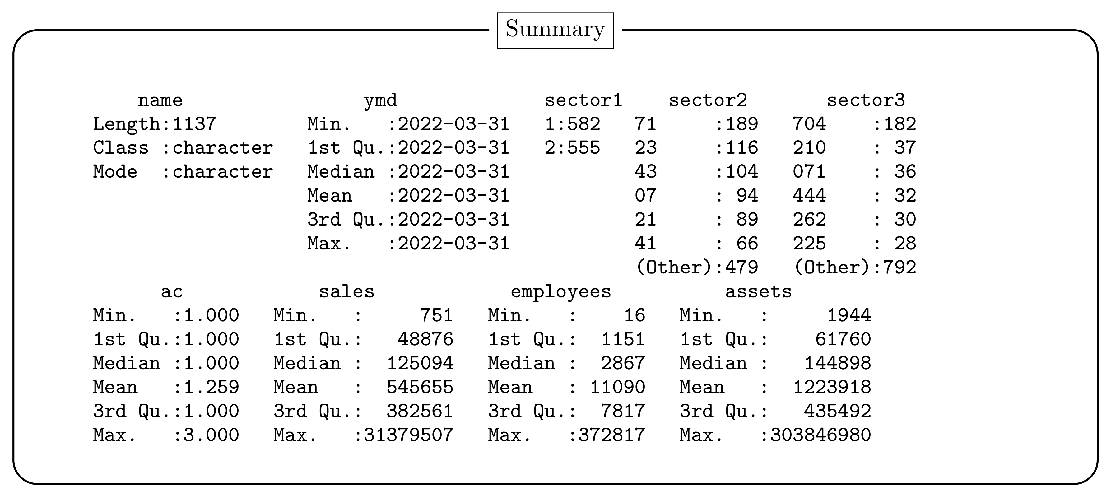
2. Data Set
- Name:
- Firm name + Nikkei Firm Code (1137 firms)
- YMD:
- Closing date
- Sector1:
- Nikkei Industry Sector Code (Major) (1: manufacture, 2: non-manufacture)
- Sector2:
- Nikkei Industry Sector Code (Middle)
- Sector3:
- Nikkei Industry Sector Code (Minor)
- AC:
- Accounting criterion (1: Japanese standard accounting, 2: United States standard accounting, 3: International Financial Reporting Standards (IFRS))
- Sales:
- Amount of sales (Unit: Million Yen)
- Employee:
- Number of employees (Unit: People)
- Assets:
- Total assets (Unit: Million Yen)
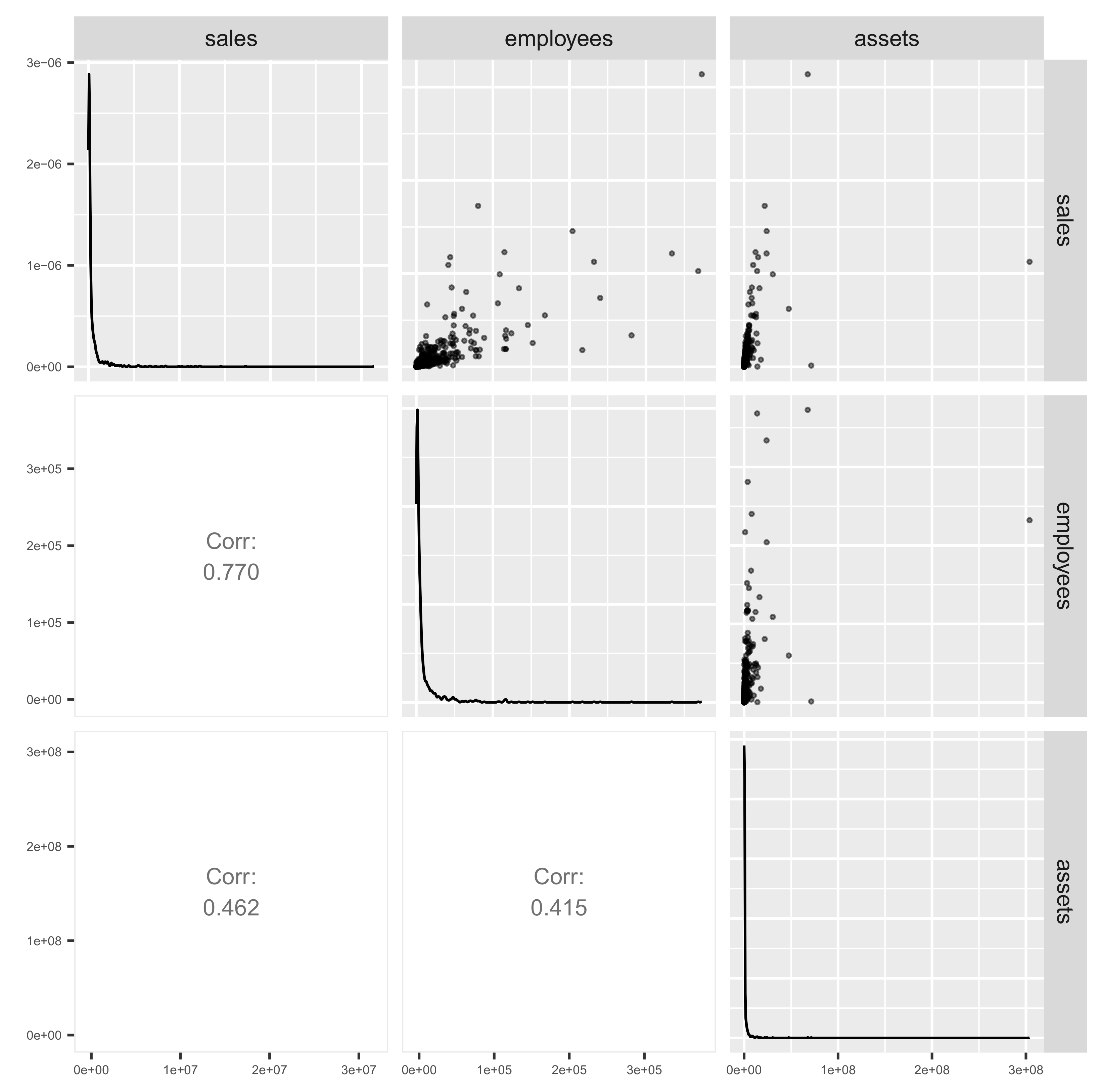
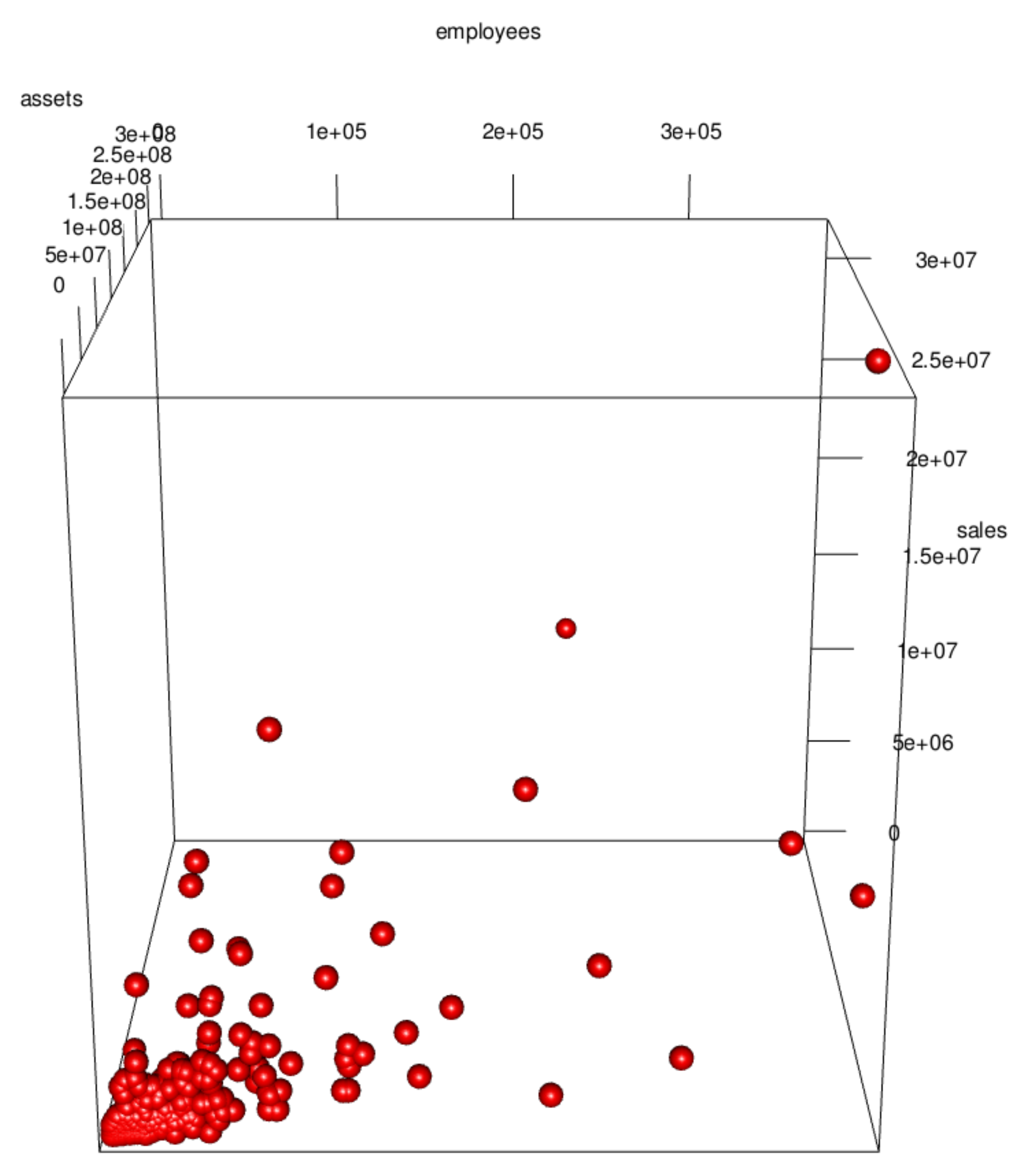
3. Data Visualization and Its Implications
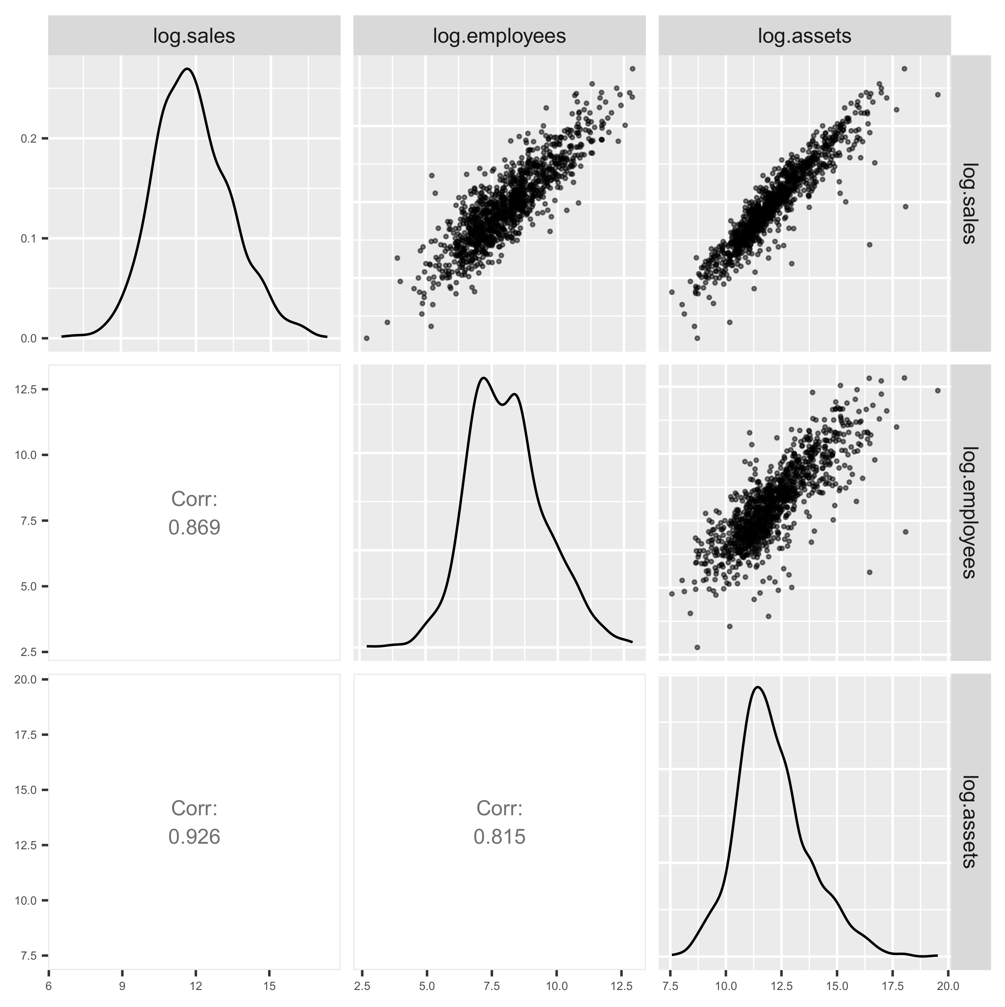
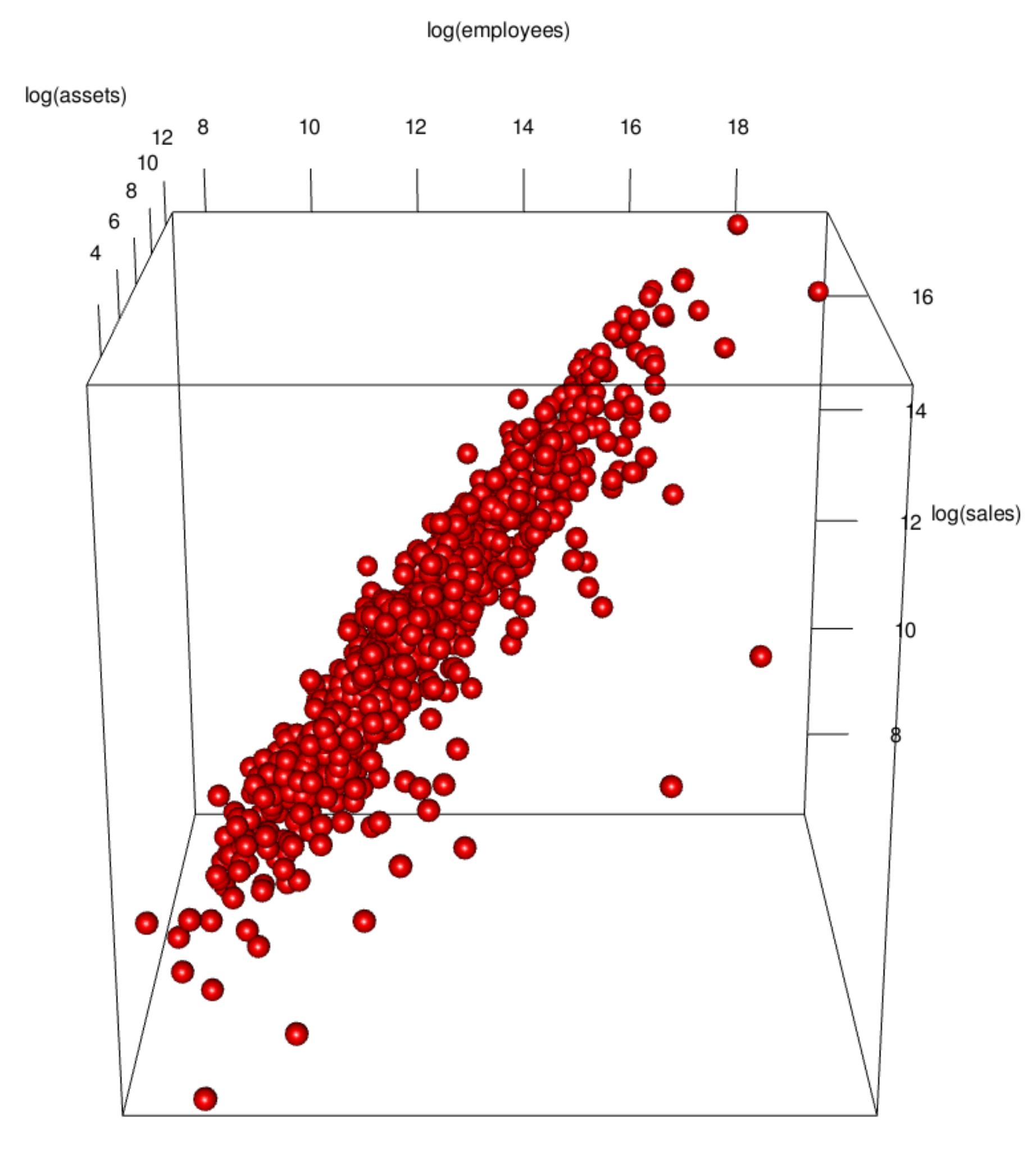
3.1. Data Visualization
3.2. Implications of Visualization
4. Regression Modeling of Cross-Sectional Data
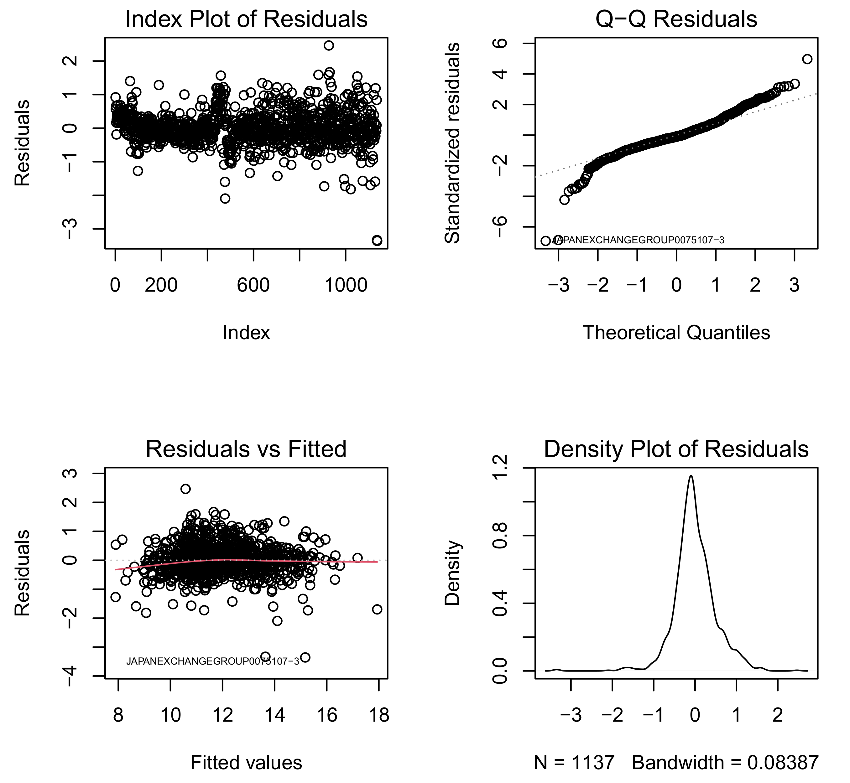
4.1. Fitting Log-Log Model with Normal Error
4.2. Fitting Log-Log Model with Skew-Normal Error
4.3. Fitting Log-Log Model with Skew-t Error
4.4. Model Selection for Log-Log Models
5. Fitting Log-Log Model with Dummy Variables
5.1. Fitting Log-Log Model with Skew-t Error and Dummy Variables
5.2. Economic Implications
5.3. Grouping ‘Insignificant’ Sectors and Final Model Comparison
6. Conclusions and Discussion
Supplementary Materials
Author Contributions
Funding
Data Availability Statement
Acknowledgments
Conflicts of Interest
Abbreviations
| AIC | Akaike Information Criterion |
| BIC | Bayesian Information Criterion |
| CP | Centered Parameter |
| DP | Direct Parameter |
| FY | Fiscal Year |
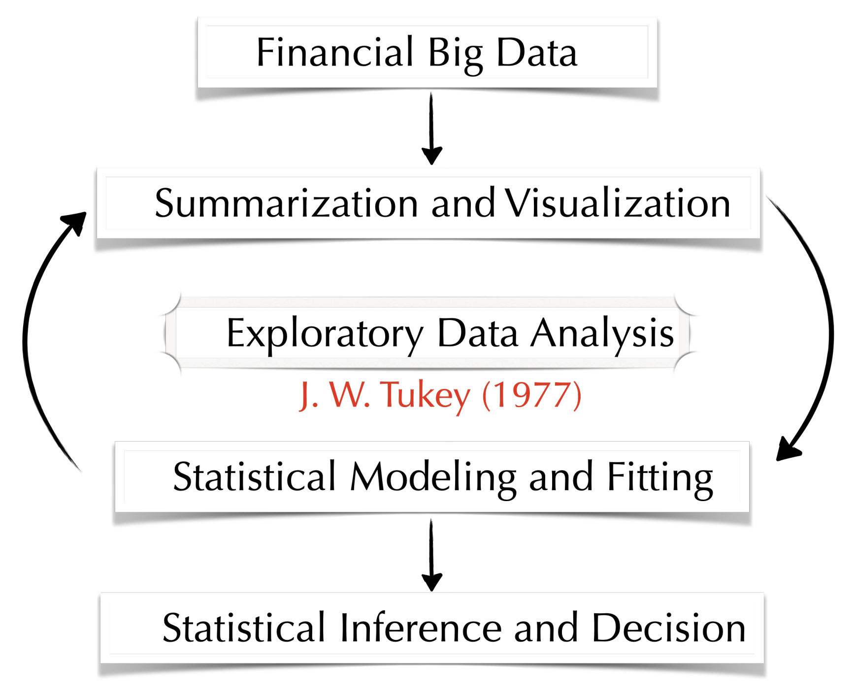
| EDA | Exploratory Data Analysis |
| MLE | Maximum Likelihood Estimate |
| TFP | Total Factor Productivity |
| TSE | Tokyo Stock Exchange |
| SN | Skew-Normal |
| ST | Skew-t |
References
- Cobb, W.C.; Douglas, P.H. A Theory of Production. Am. Econ. Rev. 1928, 18, 139–165. [Google Scholar]
- Azzalini, A. Skew-Symmetric Families of Distributions. In International Encyclopedia of Statistical Science; Lovric, M., Ed.; Springer: Berlin, Heidelberg, 2011. [Google Scholar] [CrossRef]
- Jimichi, M.; Maeda, S. Visualization and Statistical Modeling of Financial Data with R. In Proceedings of the Book of Contributed Abstracts of the International R Users Conference (useR! 2014), Los Angeles, CA, USA, 30 June–3 July 3 2014; p. 172. [Google Scholar]
- Jimichi, M. Building of Financial Database Servers; Kwansei Gakuin University: Nishinomiya, Japan, 2010; Available online: http://hdl.handle.net/10236/6013 (accessed on 9 September 2023). (In Japanese)
- Jimichi, M.; Miyamoto, D.; Saka, C.; Nagata, S. Visualization and statistical modeling of financial big data: Log-log modeling with skew-symmetric error distributions. Jpn. J. Stat. Data Sci. 2018, 1, 347–371. [Google Scholar] [CrossRef]
- Tukey, J.W. Exploratory Data Analysis; Addison-Wesley Publishing Co.: Reading, MA, USA, 1977. [Google Scholar]
- Bruce, P.; Bruce, A.; Gedeck, P. Practical Statistics for Data Scientists: 50+ Essential Concepts Using R and Python; O’Reilly Media, Inc.: Sebastopol, CA, USA, 2020. [Google Scholar]
- Wickham, H.; Grolemund, G. R for Data Science; O’Reilly: Sebastopol, CA, USA, 2016. [Google Scholar]
- Jimichi, M. Financial Data Extraction System SKWAD; Kwansei Gakuin University: Nishinomiya, Japan, 2022; Available online: http://hdl.handle.net/10236/00030225 (accessed on 9 September 2023). (In Japanese)
- Kabacoff, R.I. R in Action: Data Analysis and Graphics with R, 3rd ed.; Manning Publications Company: Shelter Island, NY, USA, 2022. [Google Scholar]
- Sievert, C. Interactive Web-Based Data Visualization with R, Plotly, and Shiny; CRC The R Series; Chapman & Hall: Boca Raton, FL, USA, 2020. [Google Scholar]
- Cook, R.D. Regression Graphics: Ideas for Studying Regressions through Graphics; John Wiley & Sons, Inc.: New York, NY, USA, 1998. [Google Scholar]
- Tufte, E.R. The Visual Display of Quantitative Information; Graphics Press: Cheshire, CT, USA, 2001. [Google Scholar]
- Wilkinson, L. The Grammar of Graphics, 2nd ed.; Springer: Chicago, IL, USA, 2005. [Google Scholar]
- Unwin, A. Graphical Data Analysis with R; CRC The R Series; Chapman & Hall: Boca Raton, FL, USA, 2015. [Google Scholar]
- Healy, K. Data Visualization: A Practical Introduction; Princeton University Press: Princeton, NJ, USA, 2018. [Google Scholar]
- Mosteller, F.; Tukey, J.W. Data Analysis and Regression: A Second Course in Statistics; Addison-Wesley: Reading, MA, USA, 1977. [Google Scholar]
- Fox, J. Applied Regression Analysis and Generalized Linear Models, 3rd ed.; SAGE Publishing: Thousand Oaks, CA, USA, 2015. [Google Scholar]
- Fox, J.; Weisbrerg, S. An R Companion to Applied Regression, 3rd ed.; SAGE Publishing: Thoutand Orks, CA, USA, 2019. [Google Scholar]
- Azzalini, A. A class of distributions which includes the normal ones. Scand. J. Stat. 1985, 12, 171–178. [Google Scholar]
- Azzalini, A.; Capitanio, A. The Skew-Normal and Related Families; Institute of Mathematical Statistics Monographs: Cambridge University Press: Cambridge, UK, 2014. [Google Scholar]
- Klein, L.R. An Introduction to Econometrics; Prentice Hall: Englewood Cliffs, NJ, USA, 1962. [Google Scholar]
- Hayashi, F. Econometrics; Princeton University Press: Princeton, NJ, USA, 2000. [Google Scholar]
- Greene, W.H. Econometric Analysis, 8th ed.; Pearson: Westford, MA, USA, 2020. [Google Scholar]
- Crow, L.E.; Shimizu, K. (Eds.) Lognormal Distributions: Theory and Applications; Marcel Dekker: Boca Raton, FL, USA, 1988. [Google Scholar]
- Kissel, R.; Poserina, J. Optimal Sports Math, Statistics, and Fantasy; Academic Press: London, UK, 2017. [Google Scholar]
- Rao, C.R. Linear Statistical Inference and Its Applications, 2nd ed.; John Wiley & Sons, Inc.: New York, NY, USA, 1973. [Google Scholar]
- Chatterjee, S.; Hadi, A.S. Sensitivity Analysis in Linear Regression; John Wiley & Sons, Inc.: New York, NY, USA, 1988. [Google Scholar]
- Cramér, H. Mathematical Methods of Statistics; Princeton University Press: Princeton, NJ, USA, 1946. [Google Scholar]
- Akaike, H. Information theory and an extension of the maximum likelihood principle. In Proceedings of the 2nd International Symposium on Information Theory, Tsahkadsor, Armenia, 2–8 September 1971; Petrov, B.N., Csaki, F., Eds.; Akadimiai Kiado: Budapest, Hungary, 1973; pp. 267–281. [Google Scholar]
- Akaike, H. On entropy maximization principle. In Applications of Statistics; Krishnaiah, P.R., Ed.; North-Holland: Amsterdam, The Neetherlands, 1977; pp. 27–41. [Google Scholar]
- Akaike, H. A Bayesian analysis of the minimum AIC procedure. Ann. Inst. Statist. Math. 1978, 30, 9–14. [Google Scholar] [CrossRef]
- Leamer, E.E. Specification Searches: Ad Hoc Inference with Non-Experimental Data; John Wiley and Sons: New York, NY, USA, 1978. [Google Scholar]
- Schwarz, G. Estimating the dimension of a model. Ann. Stat. 1978, 6, 461–464. [Google Scholar] [CrossRef]
- McNeil, A.; Frey, R.; Embrechts, P. Quantitative Risk Management: Concepts, Techniques and Tools; Revised Ed.; Princeton University Press: Princeton, NJ, USA, 2015. [Google Scholar]
- Montier, J. Behavioral Investing; John Wiley and Sons: Chichester, UK, 2007. [Google Scholar]
- Hulten, C.R. Total Factor Productivity: A Short Biography. New Developments in Productivity Analysis; Hulten, C.R., Dean, E., Harper, M., Eds.; National Bureau of Economic Research, The University of Chicago Press: Chicago, IL, USA, 2001; pp. 1–54. [Google Scholar]
- Higo, M. What caused the downward trend in Japan’s labor share? Jpn. World Econ. 2023, 67, 101206. [Google Scholar] [CrossRef]
- Leisch, F. Sweave: Dynamic generation of statistical reports using literate data analysis. In Compstat 2002, Proceedings in Computational Statistics; Härdle, W., Rönz, B., Eds.; Physica Verlag: Heidelberg, Germany, 2002; pp. 575–580. [Google Scholar]
- Mecklenburg, R. Managing Projects with GNU Make, 3rd ed.; O’Reilly Media, Inc.: Sebastopol, CA, USA, 2005. [Google Scholar]
- Peng, R.D. Reproducible research in computational science. Science 2011, 334, 1226–1227. [Google Scholar] [CrossRef] [PubMed]
- Xie, Y. Dynamic Documents with R and knitr, 2nd ed.; CRC the R Series; Chapman & Hall: Boca Raton, FL, USA, 2015. [Google Scholar]
- Gandrud, C. Reproducible Research with R and RStudio, 3rd ed.; CRC the R Series; Chapman & Hall: Boca Raton, FL, USA, 2020. [Google Scholar]


| Name | YMD | Sector1 | Sector2 | Sector3 | AC | Sales | Employees | Assets | |
|---|---|---|---|---|---|---|---|---|---|
| 1 | KYOKUYO0000001 | 31 March 2022 | 2 | 35 | 341 | 1 | 253575 | 2208 | 130460 |
| 2 | NIPPONSUISAN0000003 | 31 March 2022 | 2 | 35 | 341 | 1 | 693682 | 9662 | 505731 |
| 3 | MARUHANICHIRO0000004 | 31 March 2022 | 2 | 35 | 341 | 1 | 866702 | 12352 | 548603 |
| 4 | NITTETSUMINING0000022 | 31 March 2022 | 2 | 37 | 362 | 1 | 149082 | 2019 | 197732 |
| 5 | MITSUIMATSUSHIMAHOLDINGS0000023 | 31 March 2022 | 2 | 37 | 361 | 1 | 46592 | 1305 | 67837 |
| 6 | FURUKAWA0000043 | 31 March 2022 | 1 | 19 | 181 | 1 | 199097 | 2804 | 229727 |
| 7 | MITSUIMINING&SMELTING0000045 | 31 March 2022 | 1 | 19 | 181 | 1 | 633346 | 11881 | 637878 |
| 8 | TOHOZINC0000046 | 31 March 2022 | 1 | 19 | 181 | 1 | 124279 | 1051 | 145796 |
| 9 | MITSUBISHIMATERIALS0000047 | 31 March 2022 | 1 | 19 | 181 | 1 | 1811759 | 23711 | 2125032 |
| 10 | SUMITOMOMETALMINING0000049 | 31 March 2022 | 1 | 19 | 181 | 3 | 1259091 | 7202 | 2268756 |
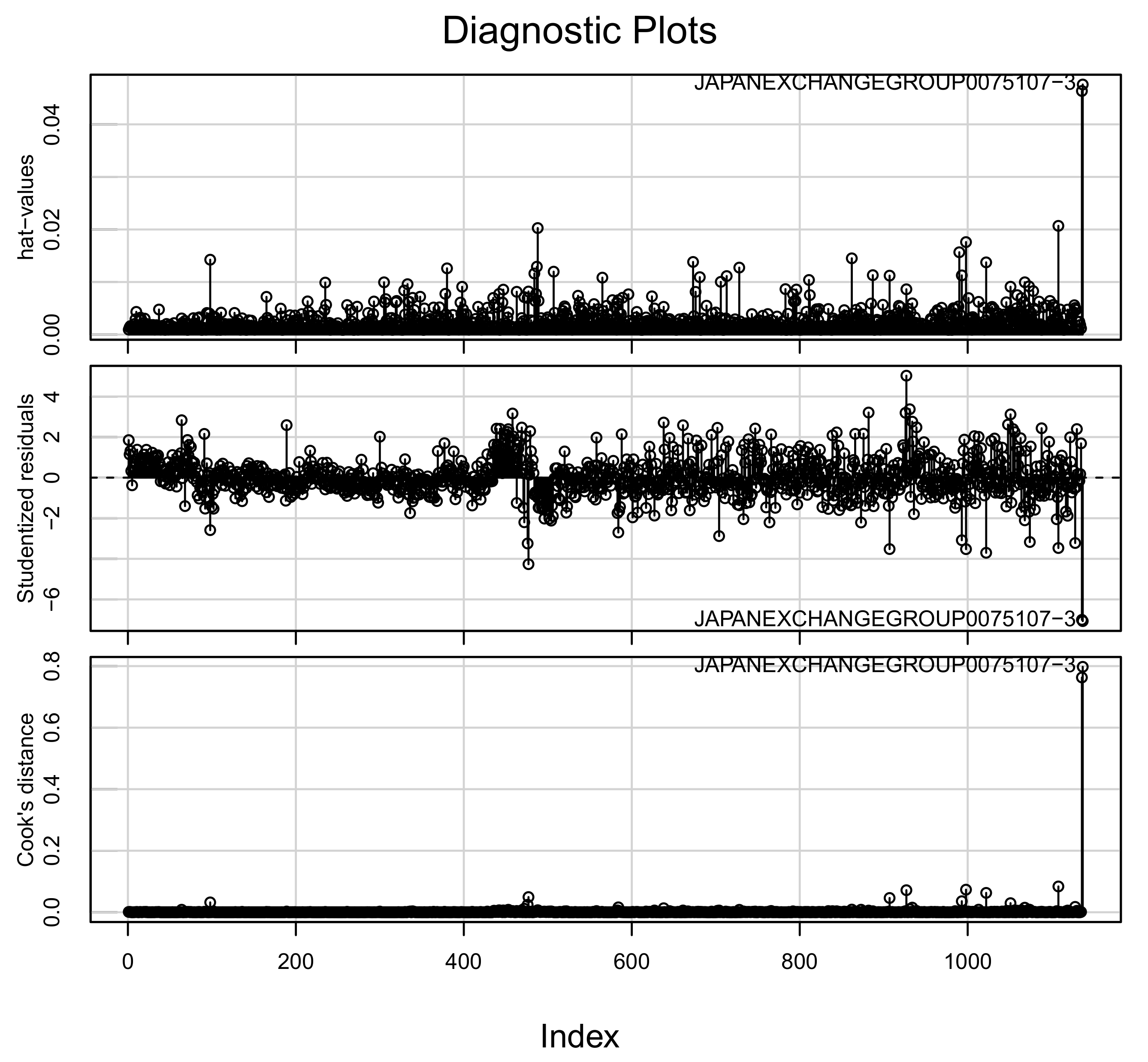
| StudRes | Hat | CookD | |
|---|---|---|---|
| TOMENDEVICES0030607-1 | 5.03 | 0.01 | 0.07 |
| JAPANPOSTHOLDINGS0038793-1 | −3.47 | 0.02 | 0.08 |
| JAPANSECURITIESFINANCE0070514-1 | −7.01 | 0.05 | 0.76 |
| JAPANEXCHANGEGROUP0075107-3 | −7.07 | 0.05 | 0.80 |
| Estimate | Std.Err | z-Ratio | Pr{>|z|} | |
|---|---|---|---|---|
| (Intercept.DP) | 1.0344 | 0.0980 | 10.56 | 0.0000 |
| log(employees) | 0.2985 | 0.0165 | 18.11 | 0.0000 |
| log(assets) | 0.6817 | 0.0150 | 45.40 | 0.0000 |
| 0.3623 | 0.0213 | 17.03 | 0.0000 | |
| 0.5435 | 0.1717 | 3.17 | 0.0016 | |
| 3.7783 | 0.4997 | 7.56 | 0.0000 |
| Dim | AIC | BIC | |
|---|---|---|---|
| Normal | 4 | 1496.43 | 1516.56 |
| Skew-Normal | 5 | 1494.69 | 1519.85 |
| Skew-t | 6 | 1397.36 | 1427.56 |
| Estimate | Std.Err | z-Ratio | Pr{>|z|} | TFP | |
|---|---|---|---|---|---|
| log(employees) | 0.2938 | 0.0157 | 18.73 | 0.0000 | — |
| log(assets) | 0.7024 | 0.0150 | 46.88 | 0.0000 | — |
| 0.2564 | 0.0158 | 16.18 | 0.0000 | — | |
| −0.5675 | 0.1853 | −3.06 | 0.0022 | — | |
| 3.5863 | 0.4394 | 8.16 | 0.0000 | — | |
| Petroleum | 0.6154 | 0.1416 | 4.35 | 0.0000 | 1.8594 |
| Wholesale Trade | 0.4497 | 0.0604 | 7.44 | 0.0000 | 1.6937 |
| Retail Trade | 0.3023 | 0.0718 | 4.21 | 0.0000 | 1.5463 |
| Fish and Marine Products | 0.2622 | 0.1422 | 1.84 | 0.0652 | 1.5062 |
| Shipbuilding and Repairing | 0.1085 | 0.2643 | 0.41 | 0.6813 | 1.3525 |
| Foods (Intercept.DP) | 1.3660 | 0.1057 | 12.92 | 0.0000 | 1.2440 |
| Construction | −0.0029 | 0.0588 | −0.05 | 0.9605 | 1.2411 |
| Iron and Steel | −0.1624 | 0.0730 | −2.22 | 0.0261 | 1.0816 |
| Warehousing and Harbor Transportation | −0.2067 | 0.1117 | −1.85 | 0.0644 | 1.0373 |
| Sea Transportation | −0.2110 | 0.1273 | −1.66 | 0.0973 | 1.0330 |
| Non-Ferrous Metal and Metal Products | −0.2252 | 0.0674 | −3.34 | 0.0008 | 1.0188 |
| Utilities—Gas | −0.2267 | 0.1132 | −2.00 | 0.0452 | 1.0173 |
| Real Estate | −0.2507 | 0.0924 | −2.71 | 0.0067 | 0.9933 |
| Mining | −0.2623 | 0.1424 | −1.84 | 0.0655 | 0.9817 |
| Pulp and Paper | −0.2710 | 0.0912 | −2.97 | 0.0030 | 0.9730 |
| Trucking | −0.2751 | 0.0840 | −3.28 | 0.0010 | 0.9689 |
| Motor Vehicles and Auto Parts | −0.2935 | 0.0640 | −4.59 | 0.0000 | 0.9505 |
| Other Manufacturing | −0.3027 | 0.0770 | −3.93 | 0.0001 | 0.9413 |
| Services | −0.3048 | 0.0555 | −5.49 | 0.0000 | 0.9392 |
| Transportation Equipment | −0.3107 | 0.1125 | −2.76 | 0.0058 | 0.9333 |
| Chemicals | −0.3284 | 0.0562 | −5.84 | 0.0000 | 0.9156 |
| Communication Services | −0.4065 | 0.0943 | −4.31 | 0.0000 | 0.8375 |
| Stone, Clay, and Glass Products | −0.4198 | 0.0756 | −5.55 | 0.0000 | 0.8242 |
| Electric and Electronic Equipment | −0.4450 | 0.0561 | −7.94 | 0.0000 | 0.7990 |
| Machinery | −0.4734 | 0.0567 | −8.36 | 0.0000 | 0.7706 |
| Rubber Products | −0.4754 | 0.1016 | −4.68 | 0.0000 | 0.7686 |
| Drugs | −0.4848 | 0.0706 | −6.86 | 0.0000 | 0.7592 |
| Precision Equipment | −0.5204 | 0.0716 | −7.27 | 0.0000 | 0.7236 |
| Textile Products | −0.5943 | 0.0868 | −6.85 | 0.0000 | 0.6497 |
| Utilities—Electric | −0.6013 | 0.0900 | −6.68 | 0.0000 | 0.6427 |
| Credit and Leasing | −0.8536 | 0.1031 | −8.28 | 0.0000 | 0.3904 |
| Railroad Transportation | −1.0878 | 0.0749 | −14.52 | 0.0000 | 0.1562 |
| Air Transportation | −1.1681 | 0.1623 | −7.20 | 0.0000 | 0.0759 |
| Dim | AIC | BIC | |
|---|---|---|---|
| Distinct Sector Dummies Only | 34 | 4013.01 | 4184.12 |
| Log-Log Normal/w DSDs | 36 | 840.75 | 1021.93 |
| Log-Log Skew-Normal/w DSDs | 37 | 820.13 | 1006.33 |
| Log-Log Skew-t/w DSDs | 38 | 701.23 | 892.47 |
| Log-Log Skew-t/w PGSDs | 31 | 704.14 | 860.15 |
Disclaimer/Publisher’s Note: The statements, opinions and data contained in all publications are solely those of the individual author(s) and contributor(s) and not of MDPI and/or the editor(s). MDPI and/or the editor(s) disclaim responsibility for any injury to people or property resulting from any ideas, methods, instructions or products referred to in the content. |
© 2023 by the authors. Licensee MDPI, Basel, Switzerland. This article is an open access article distributed under the terms and conditions of the Creative Commons Attribution (CC BY) license (https://creativecommons.org/licenses/by/4.0/).
Share and Cite
Jimichi, M.; Kawasaki, Y.; Miyamoto, D.; Saka, C.; Nagata, S. Statistical Modeling of Financial Data with Skew-Symmetric Error Distributions. Symmetry 2023, 15, 1772. https://doi.org/10.3390/sym15091772
Jimichi M, Kawasaki Y, Miyamoto D, Saka C, Nagata S. Statistical Modeling of Financial Data with Skew-Symmetric Error Distributions. Symmetry. 2023; 15(9):1772. https://doi.org/10.3390/sym15091772
Chicago/Turabian StyleJimichi, Masayuki, Yoshinori Kawasaki, Daisuke Miyamoto, Chika Saka, and Shuichi Nagata. 2023. "Statistical Modeling of Financial Data with Skew-Symmetric Error Distributions" Symmetry 15, no. 9: 1772. https://doi.org/10.3390/sym15091772
APA StyleJimichi, M., Kawasaki, Y., Miyamoto, D., Saka, C., & Nagata, S. (2023). Statistical Modeling of Financial Data with Skew-Symmetric Error Distributions. Symmetry, 15(9), 1772. https://doi.org/10.3390/sym15091772