On a Measure of Tail Asymmetry for the Bivariate Skew-Normal Copula

Abstract

Asymmetry in the upper and lower tails is an important feature in modeling bivariate distributions. This article focuses on the log ratio between the tail probabilities at upper and lower corners as a measure of tail asymmetry. Asymptotic behavior of this measure at extremely large and small thresholds is explored with particular emphasis on the skew-normal copula. Our numerical studies reveal that, when the correlation or skewness parameters are around at the boundary values, some asymptotic tail approximations of the skew-normal copulas proposed in the literature are not suitable to compute the measure of tail asymmetry with practically extremal thresholds.

1. Introduction

Skewness in data is an important feature in various applications. As a typical example, dependence among stock returns is known to be asymmetric in bearish and bullish markets [1]. To capture such asymmetry, skewed multivariate distributions have been extensively studied in the literature. A popular family of skewed distributions is the skew-elliptical distribution [2], which includes, for example, the skew-normal distribution [3] and the skew-t distribution [4]. These models capture different features of asymmetry especially in their tails. To find an appropriate model for given data, it is important to quantify the degrees of tail asymmetry in the data and models. A mismatch of such a feature may lead to erroneous results in the statistical analysis. Therefore, evaluating the degree of tail asymmetry is an essential task to carry out decent statistical analysis. In this regard, various measures of asymmetry have been proposed to quantify certain asymmetric features of an underlying distribution. See, for example, refs. [5,6,7,8,9] for such measures for bivariate distributions.

In this paper, we focus on the skew-normal distribution, which is known to be beneficial for flexibly modeling an asymmetric feature of data especially between the degrees of upper and lower tail dependence. A d-dimensional random vector $\mathbf{Y}=(Y_1,\cdots ,Y_n)$ is said to follow the skew-normal distribution, denoted by $\mathbf{Y}\sim {SN}_d(\delta ,\mathsf{\Psi })$, if it admits the stochastic representation

$$\begin{array}{c}\hfill Y_j={\delta }_j\left|Z_0\right|+\sqrt{1-{\delta }_j^2}{Z}_j,{\delta }_j\in (-1,1),\mathsf{\Psi }\in {\mathcal{P}}_d,\end{array}$$

(1)

where $Z_0\sim N(0,1)$, $\mathbf{Z}=(Z_1,\cdots ,Z_d)\sim N_d(\mathbf{0},\mathsf{\Psi })$ is independent of $Z_0$ and ${\mathcal{P}}_d$ is a set of all d-dimensional correlation matrices. The parameter $\delta =({\delta }_1,\cdots ,{\delta }_d)\in {(-1,1)}^d$ is called the skewness parameter and $\mathsf{\Psi }\in {\mathcal{P}}_d$ is called the correlation matrix. The skew-normal copula, denoted by $C_{SN}(·;\delta ,\mathsf{\Psi })$, is defined as the copula of $\mathbf{Y}\sim {SN}_d(\delta ,\mathsf{\Psi })$. The reader is referred to [10] for statistical applications of the skew-normal distribution and [2,11,12] for recent overview of skew-normal and related distributions. An important feature of the skew-normal copula is that the tail orders introduced in [13] are allowed to be different in the upper and lower tails; see, for example, [14].

The difference of tail orders between upper and lower tails is not properly captured by some measures of tail asymmetry proposed in the literature. One of the most prevalent measures of tail dependence is the tail dependence coefficient (TDC) [15,16]. Let H be a bivariate cumulative distribution function (cdf) of $\mathbf{X}=(X_1,X_2)$ with continuous marginal distributions $F_1$ and $F_2$, respectively. The lower and upper TDCs for H are defined, respectively, by 

$$\begin{array}{c}\hfill {\lambda }_L\left(H\right)=\underset{u\downarrow 0}{lim}{\lambda }_L\left(u\right)\mathrm{and}{\lambda }_U\left(H\right)=\underset{u\downarrow 0}{lim}{\lambda }_U\left(u\right),\end{array}$$

where ${\lambda }_L$ and ${\lambda }_U$ are the lower and upper tail dependence functions defined by

$$\begin{array}{cc}\hfill {\lambda }_L\left(u\right)& =\mathbb{P}(X_1\le F_1^{-1}\left(u\right)\mid X_2\le F_2^{-1}\left(u\right))\mathrm{and}\hfill \\ \hfill {\lambda }_U\left(u\right)& =\mathbb{P}(X_1\ge F_1^{-1}(1-u)\mid X_2\ge F_2^{-1}(1-u)),\hfill \end{array}$$

respectively. Note that ${\lambda }_L\left(u\right)=C(u,u)/u$ and ${\lambda }_U\left(u\right)=\overline{C}(1-u,1-u)/u$ where C is the cdf of $(U_1,U_2)=(F_1\left(X_1\right),F_2\left(X_2\right))$ called the copula of $\mathbf{X}$, and $\overline{C}(u_1,u_2)=\mathbb{P}(U_1\ge u_1,U_2\ge u_2)$, $(u_1,u_2)\in {[0,1]}^2$. The TDCs have been studied for various skew bivariate distribution, such as the skew-normal distribution [14,17,18], the skew-t or skew-slash distribution [19,20,21,22,23], and the skew-Laplace and skew-Cauchy distribution [24]. Due to the popularity of the TDCs, it is tempting to quantify the measure of tail asymmetry by the difference between the upper and lower TDCs. In fact, many existing measures are based on differences between certain measures of upper and lower tails (see, e.g., [5,6,7,8]). Such difference-based measures are typically appropriate when the tail orders are equal between upper and lower tails, which is the case for the skew-t, skew-slash, and skew-Cauchy distributions. On the other hand, such difference-based measures are sometimes inappropriate to quantify tail asymmetry of the skew-normal copula since values of these measures tend to be small even for large values of $\left|\right|\delta \left|\right|$. For example, the upper and lower TDCs of the skew-normal copula are typically zero, and thus their difference is zero even in the presence of strong skewness.

To quantify the degree of difference of tail orders between upper and lower tails, we focus on a log-difference-based measure of tail asymmetry proposed by [9]. For a more formal description, let $\mathbf{X}=(X_1,X_2)$ be an ${\mathbb{R}}^2$-valued random vector on a fixed atomless probability space. Denote by H the cumulative distribution function (cdf) of $\mathbf{X}$ with marginal distributions $F_1$ and $F_2$, respectively. For a fixed threshold $u\in (0,1/2]$, Ref. [9] proposed the measure of tail asymmetry (in lower and upper tails) defined by

$$\begin{array}{c}\hfill {\alpha }_H\left(u\right)=log\left(\frac{\mathbb{P}(X_1\ge F_1^{-1}(1-u),X_2\ge F_2^{-1}(1-u))}{\mathbb{P}(X_1\le F_1^{-1}\left(u\right),X_2\le F_2^{-1}\left(u\right))}\right).\end{array}$$

(2)

We are also interested in the asymptotic behavior of ${\alpha }_H\left(u\right)$ as $u\downarrow 0$. Throughout the paper, we assume that $F_1$ and $F_2$ are continuous so that $(X_1,X_2)$ has the unique copula C. Then, ${\alpha }_H$ is a function of the copula given by

$$\begin{array}{cc}\hfill {\alpha }_H\left(u\right)& =log\left(\frac{\mathbb{P}(U_1\ge 1-u,U_2\ge 1-u)}{\mathbb{P}(U_1\le u,U_2\le u)}\right)\hfill \\ \hfill & =log\left(\frac{\overline{C}(1-u,1-u)}{C(u,u)}\right)=:{\alpha }_C\left(u\right).\hfill \end{array}$$

(3)

The measure (2) returns reasonable values because this measure is based on the ratio between upper and lower tail probabilities. To the best of our knowledge, the measure (2) is the only ratio-based measure of upper and lower tail probabilities, which seems appropriate to measure the tail asymmetry of the skew-normal copula. Note that the measure ${\alpha }_C\left(u\right)$ in (3) is also represented by the lower and upper tail dependence functions as ${\alpha }_C\left(u\right)={\lambda }_U\left(u\right)/{\lambda }_L\left(u\right)$. When the upper and lower TDCs are well-defined as positive values, we have that ${lim}_{u\downarrow 0}{\alpha }_C\left(u\right)={\lambda }_U/{\lambda }_L$, and thus the results in [19,20,21,22,23,24] are applicable to compute the limit of ${\alpha }_C\left(u\right)$.

The contribution of this paper is twofold. First, we derive an asymptotic formula of the measure of tail asymmetry (2) in terms of the upper and lower tail orders [13]. This formula enables us to describe the asymptotic behavior of this measure for the skew-normal copula. Various approaches are also introduced to evaluate the measure (2) for a finite threshold $u\in (0,1/2]$. Our second contribution is to numerically demonstrate that, when the correlation or skewness parameters are around at the boundary values, some asymptotic formulas of the skew-normal copula proposed in the literature are not suitable to compute the measure of tail asymmetry with practically extremal thresholds, such as $u=0.01$. This finding supports the use of an exact evaluation of the measure (2) even for an extremely small threshold $u\in (0,1/2]$ instead of some asymptotic tail approximations proposed in the literature.

The organization of this paper is as follows. In Section 2, we review the concept of tail order and skew-normal copulas. In Section 3, we derive a formula of the measure of tail asymmetry in terms of the upper and lower tail orders. We also explore the measure and its asymptotic behavior for the skew-normal copula. Numerical experiments are provided in Section 4, where we reveal some situations when some asymptotic formulas of the skew-normal copula proposed in the literature are not appropriate to use. Section 5 concludes this paper. Detailed calculations and all proofs are deferred to Appendix A and Appendix B, respectively.

2. Preliminaries

We begin with introducing some concepts and notations. Two functions $f,g:\mathbb{R}\to \mathbb{R}$ are called asymptotically equivalent at $a\in \overline{\mathbb{R}}=\mathbb{R}\cup \{\pm \infty \}$, denoted by $f\left(x\right)\sim g\left(x\right)$, $x\to a$, if ${lim}_{x\to a}f\left(x\right)/g\left(x\right)=1$. A function $f:\mathbb{R}\to \mathbb{R}$ is called slowly varying at $a\in [0,\infty ]$ if ${lim}_{x\to a}f\left(tx\right)/f\left(x\right)=1$ for any $t\in (0,\infty )$. The set of all slowly varying functions at a is denoted by ${SV}_a$. Throughout the paper, all vectors in the form $(x_1,\cdots ,x_n)$, $n\in \mathbb{N}$, are understood as column vectors.

2.1. Tail Order and Tail Order Parameter

According to [13], a d-dimensional copula C is said to have the lower tail order ${\kappa }_L\left(C\right)\ge 1$ if

$$\begin{array}{c}\hfill C(u,\cdots ,u)\sim u^{{\kappa }_L\left(C\right)}{\ell }_L\left(u\right),u\downarrow 0,\end{array}$$

(4)

where ${\ell }_L\in {SV}_0$. If, in addition, the limit ${lim}_{u\downarrow 0}{\ell }_L\left(u\right)={\ell }_L^{*}\left(C\right)$ exists, then C is said to have the lower tail order parameter${\ell }_L^{*}\left(C\right)\in [0,\infty ]$. The copula C is called (lower) tail dependent when ${\kappa }_L\left(C\right)=1$. In this case, ${\ell }_L^{*}\left(C\right)$ is known as the (lower) tail dependence coefficient (TDC). The case ${\kappa }_L\left(C\right)=d$ is referred to as the tail independence. When $1<{\kappa }_L\left(C\right)<d$, C is said to have intermediate tail dependence. As such the model (4) can capture weaker tail dependence that the TDC cannot. Similarly to the lower case, C is said to have the upper tail order${\kappa }_U\left(C\right)\ge 1$ and the upper tail order parameter${\ell }_U^{*}\left(C\right)\in [0,\infty ]$ if

$$\begin{array}{c}\hfill \overline{C}(1-u,\cdots ,1-u)\sim u^{{\kappa }_U\left(C\right)}{\ell }_U\left(u\right),u\downarrow 0,\end{array}$$

(5)

where ${\ell }_U\in {SV}_0$ is such that ${lim}_{u\downarrow 0}{\ell }_U\left(u\right)={\ell }_U^{*}\left(C\right)$.

2.2. The Skew-Normal Copula

Let $\mathbf{Y}\sim {SN}_d(\delta ,\mathsf{\Psi })$ follow a d-dimensional skew-normal distribution defined via the stochastic representation (1). According to [3], the joint probability density functions (pdf) of $\mathbf{Y}$ is given by

$$\begin{array}{cc}\hfill f_{SN}(\mathbf{y};\tilde{\mathit{\alpha }},\mathsf{\Omega })& =2{\varphi }_d(\mathbf{y};\mathsf{\Omega })\mathsf{\Phi }\left({\tilde{\mathit{\alpha }}}^{\top }\mathbf{y}\right),\mathbf{y}\in {\mathbb{R}}^d,\hfill \end{array}$$

where ${\varphi }_d(·;\mathsf{\Omega })$ is the pdf of $N_d(\mathbf{0},\mathsf{\Omega })$ and the parameters $\mathsf{\Omega }\in {\mathcal{P}}^d$ and $\tilde{\alpha }\in {\mathbb{R}}^d$ are specified via

$$\begin{array}{cc}\hfill \mathsf{\Omega }& =\Delta (\mathsf{\Psi }+\zeta {\zeta }^{\top })\Delta ,\hfill \end{array}$$

(6)

$$\begin{array}{cc}\hfill \tilde{\alpha }& =\frac{{\mathsf{\Omega }}^{-1}\delta }{\sqrt{1-{\delta }^{\top }{\mathsf{\Omega }}^{-1}\delta }}=\frac{{\Delta }^{-1}{\mathsf{\Psi }}^{-1}\zeta }{\sqrt{1+{\zeta }^{\top }{\mathsf{\Psi }}^{-1}\zeta }},\hfill \end{array}$$

(7)

where

$$\begin{array}{cc}\hfill \Delta & =diag\left(\sqrt{1-{\delta }_1^2},\cdots ,\sqrt{1-{\delta }_d^2}\right),\hfill \\ \hfill \zeta & =({\zeta }_1,\cdots ,{\zeta }_d),{\zeta }_j=\frac{{\delta }_j}{\sqrt{1-{\delta }_j^2}},j\in \{1,\cdots ,d\}.\hfill \end{array}$$

The marginal pdf of $Y_j$, $j\in \{1,\cdots ,d\}$, is given by

$$\begin{array}{cc}\hfill f_{SN}(y_j;{\delta }_j)& =2\varphi \left(y_j\right)\mathsf{\Phi }\left({\zeta }_j{y}_j\right),y_j\in \mathbb{R},\hfill \end{array}$$

where $\varphi$ and $\mathsf{\Phi }$ are pdf and cdf of $N(0,1)$, respectively. Note that $Y_j\sim SN\left({\delta }_j\right)$, $j\in \{1,\cdots ,d\}$, where $SN\left({\delta }_j\right)={SN}_1({\delta }_j,1)$. Moreover, it follows from (1) that

$$\begin{array}{c}\hfill -\mathbf{Y}\sim {SN}_d(-\delta ,\mathsf{\Psi }).\end{array}$$

(8)

Skewness of the skew-normal copula is illustrated in Figure 1, where the contour plot of the (symmetric) normal distribution is compared with that of the skew-normal copula with its marginal distributions transformed into the standard normal distributions.

Figure 1. Contour plots of the (symmetric) normal distribution with $\rho =0.5$ (left) and the skew-normal copula $C_{SN}(\delta ,\mathsf{\Psi })$ with $({\delta }_1,{\delta }_2,{\mathsf{\Psi }}_{1,2})=(-0.8,-0.8,0.5)$ with its marginal distributions transformed into the standard normal distributions (right).

The skew-normal distribution can be written in terms of the conditional distribution of the normal distribution. More precisely, it is shown in Section 2.2 of [3] that

$$\begin{array}{c}\hfill (X_1,\cdots ,X_d)\mid \{X_0>0\}\sim {SN}_d(\delta ,\mathsf{\Psi }),\end{array}$$

(9)

where $(X_0,X_1,\cdots ,X_d)\sim N_{d+1}({\mathbf{0}}_{d+1},{\mathsf{\Omega }}^{*}\left(\delta \right))$ with the extended correlation matrix

$$\begin{array}{c}\hfill {\mathsf{\Omega }}^{*}\left(\delta \right)=\left(\begin{array}{cc}1& {\delta }^{\top }\\ \delta & \mathsf{\Omega }\end{array}\right)\in {\mathcal{P}}_{d+1}.\end{array}$$

(10)

This representation allows us to write the cdfs of ${SN}_d(\delta ,\mathsf{\Psi })$ and its copula as follows.

Lemma 1. 

Let $F_{SN}(·;\delta ,\mathsf{\Psi })$ be the cdf of $\mathbf{Y}\sim {SN}_d(\delta ,\mathsf{\Psi })$ with marginal cdfs $F_{SN}(·;{\delta }_j)$, $j\in \{1,\cdots ,d\}$. Then

$$\begin{array}{c}\hfill F_{SN}(\mathbf{y};\delta ,\mathsf{\Psi })=2{\mathsf{\Phi }}_{d+1}((0,\mathbf{y});{\mathsf{\Omega }}^{*}(-\delta )),\end{array}$$

(11)

where ${\mathsf{\Phi }}_{d+1}(·;{\mathsf{\Omega }}^{*}(-\delta ))$ is the cdf of $N_{d+1}({\mathbf{0}}_{d+1},{\mathsf{\Omega }}^{*}(-\delta ))$. Therefore, the cdf of the skew-normal copula $C_{SN}(·;\delta ,\mathsf{\Psi })$ can be written by

$$\begin{array}{c}\hfill C_{SN}(\mathbf{u};\delta ,\mathsf{\Psi })=2{\mathsf{\Phi }}_{d+1}((0,F_{SN}^{-1}(u_1;{\delta }_1),\cdots ,F_{SN}^{-1}(u_d;{\delta }_d));{\mathsf{\Omega }}^{*}(-\delta )).\end{array}$$

(12)

3. Tail Asymmetry of the Skew-Normal Copula

In this section, we explore tail asymmetry of the skew-normal copula via the measure (2) and its asymptotic behavior. We will show in Proposition 1 that the measure (2), after properly scaled, quantifies the difference between the upper and lower tail orders when they differ. Moreover, when the upper and lower tail orders coincide, the measure (2) quantifies the difference between the upper and lower tail order parameters. These results support the use of the measure (2) for quantifying tail asymmetry of the skew-normal copula since, to our knowledge, difference-based measures of asymmetry proposed in the literature do not measure tail asymmetry properly when the upper and lower tail indices are not equal.

3.1. Measure of Tail Asymmetry and Tail Order

This section explores the relationship between the measure of tail asymmetry (2) and the tail order. To this end, suppose that a bivariate copula C satisfies (4) and (5).

The next proposition states that the measure of tail asymmetry (2) can be asymptotically represented in terms of the difference between the upper and lower tail indices.

Proposition 1 

(Measure of tail asymmetry and tail order). Let C be a bivariate copula with lower and upper tail orders ${\kappa }_L\left(C\right)$ and ${\kappa }_U\left(C\right)$, respectively. If ${\kappa }_U\left(C\right)\ne {\kappa }_L\left(C\right)$, then

$$\begin{array}{c}\hfill {\alpha }_C\left(u\right)\sim \{{\kappa }_U\left(C\right)-{\kappa }_L\left(C\right)\}logu,u\downarrow 0.\end{array}$$

(13)

If ${\kappa }_U\left(C\right)={\kappa }_L\left(C\right)$ and C admits the upper and lower tail order parameters ${\ell }_U^{*}\left(C\right),{\ell }_L^{*}\left(C\right)\in (0,\infty )$, then

$$\begin{array}{c}\hfill {\alpha }_C\left(u\right)\sim log\left(\frac{{\ell }_U^{*}\left(C\right)}{{\ell }_L^{*}\left(C\right)}\right).\end{array}$$

(14)

Remark 1 

(Relationship with TDCs). Equation (14) implies that the limit of ${\alpha }_C\left(u\right)$ as $u\downarrow 0$ is obtainable from upper and lower TDCs. Indeed, if ${\kappa }_U\left(C\right)={\kappa }_L\left(C\right)=1$, ${\ell }_U^{*}\left(C\right)$ and ${\ell }_L^{*}\left(C\right)$ correspond to upper and lower TDCs, respectively. Then ${lim}_{u\downarrow 0}{\alpha }_C\left(u\right)$ is a straightforward calculation from (14). This result can be applied to evaluate the limit of ${\alpha }_C\left(u\right)$ of, for example, the skew-t distribution, whose upper and lower TDCs are available; see [19].

3.2. Measure of Tail Asymmetry of the Skew-Normal Copula

From this section, we focus on the bivariate case $d=2$. Let $\tilde{\rho }\in (-1,1)$ be the off-diagonal entry of $\mathsf{\Psi }$ and $\rho \in (-1,1)$ be that of $\mathsf{\Omega }$. We denote, for example, the bivariate case of $C_{\mathrm{SN}}(·;\delta ,\mathsf{\Psi })$ by $C_{\mathrm{SN}}(·;\delta ,\tilde{\rho })$ for notational simplicity. Note that $\tilde{\rho }$ is the partial correlation of $Y_1$ and $Y_2$ given $Z_0$, where $Z_0,Y_1$ and Y are those used in (1). By calculation, it holds that

$$\begin{array}{c}\hfill \rho =\tilde{\rho }\sqrt{(1-{\delta }_1^2)(1-{\delta }_2^2)}+{\delta }_1{\delta }_2.\end{array}$$

(15)

By selecting $({\delta }_1,{\delta }_2)\in {(-1,1)}^2$ and $\tilde{\rho }\in (-1,1)$ independently, the range of the parameter $\rho$ implied by (15) is given by    

$$\begin{array}{c}\hfill {\delta }_1{\delta }_2-\sqrt{(1-{\delta }_1^2)(1-{\delta }_2^2)}<\rho <{\delta }_1{\delta }_2+\sqrt{(1-{\delta }_1^2)(1-{\delta }_2^2)}.\end{array}$$

(16)

Moreover, in the bivariate case, the parameter $\tilde{\alpha }$ is given by

$$\begin{array}{c}\hfill \tilde{\alpha }=\frac{1}{\sqrt{(1-{\rho }^2)(1-{\tilde{\rho }}^2)(1-{\delta }_1^2)(1-{\delta }_2^2)}}\left(\begin{array}{c}{\delta }_1-\rho {\delta }_2\\ {\delta }_2-\rho {\delta }_1\end{array}\right).\end{array}$$

(17)

The reader is referred to Appendix A.1 for detailed derivations of (15) and (17).

We first consider the case of a finite threshold $u\in (0,1/2]$. In this case, the measure of tail asymmetry (2) of the skew-normal copula can be evaluated by the following proposition. Note that we denote by ${\alpha }_{SN}(u;\delta ,\tilde{\rho })$ the measure (2) of the skew-normal copula $C_{SN}(·;\delta ,\tilde{\rho })$.

Proposition 2 

(Measure of tail asymmetry of the skew-normal copula). Let $C_{SN}(·;\delta ,\tilde{\rho })$ be the skew-normal copula with $\delta \in {(-1,1)}^2$ and $\tilde{\rho }\in (-1,1)$. Then, its measure of tail asymmetry (2) for a finite threshold $u\in (0,1/2]$ is given by

$$\begin{array}{cc}\hfill {\alpha }_{SN}(u;\delta ,\tilde{\rho })& =log\left(\frac{C_{SN}(u,u;-\delta ,\tilde{\rho })}{C_{SN}(u,u;\delta ,\tilde{\rho })}\right)\hfill \\ \hfill & =log\left(\frac{{\mathsf{\Phi }}_3\left((0,F_{SN}^{-1}(u;-{\delta }_1),F_{SN}^{-1}(u;-{\delta }_2));{\mathsf{\Omega }}^{*}\left(\delta \right)\right)}{{\mathsf{\Phi }}_3\left((0,F_{SN}^{-1}(u;{\delta }_1),F_{SN}^{-1}(u;{\delta }_2));{\mathsf{\Omega }}^{*}(-\delta )\right)}\right),\hfill \end{array}$$

(18)

where

$$\begin{array}{c}\hfill {\mathsf{\Omega }}^{*}\left(\delta \right)=\left(\begin{array}{ccc}1& {\delta }_1& {\delta }_2\\ {\delta }_1& 1& \tilde{\rho }\sqrt{1-{\delta }_1^2}\sqrt{1-{\delta }_2^2}+{\delta }_1{\delta }_2\\ {\delta }_2& \tilde{\rho }\sqrt{1-{\delta }_1^2}\sqrt{1-{\delta }_2^2}+{\delta }_1{\delta }_2& 1\end{array}\right).\end{array}$$

The Formula (18) enables us to numerically compute ${\alpha }_{SN}(u;\delta ,\tilde{\rho })$ for a finite threshold $u\in (0,1/2]$.

For an illustrative example, Figure 2 provides curves of ${\alpha }_{SN}(u;\delta ,\tilde{\rho })$, $u=0.01$, for the skew-normal copula with different parameters. The function ${\mathsf{\Phi }}_3$ in (18) is evaluated by pmvnorm(algorithm = TVPACK) [25] in the R package mvtnorm. We observe that the measure ${\alpha }_{SN}(u;\delta ,\tilde{\rho })$ is symmetric in $\delta$ with respect to $\delta =0$ and is monotonically changing in $\tilde{\rho }$.

Figure 2. The measure of tail asymmetry ${\alpha }_{SN}(u;\delta ,\tilde{\rho })$, $u=0.01$, for different parameters of the skew-normal copula with ${\delta }_1={\delta }_2=\delta$.

We next consider the asymptotic behavior of $\alpha \left(u\right)$ for an extremely large and small thresholds. Summarizing the existing results in the literature, we have that

$$\begin{array}{c}\hfill {\kappa }_L(C_{SN};\delta ,\tilde{\rho })=\left\{\begin{array}{cc}\frac{2}{1+\tilde{\rho }},\hfill & \mathrm{if}{\delta }_1,{\delta }_2\ge 0,\hfill \\ \frac{2}{1+\rho },\hfill & \mathrm{if}{\delta }_1,{\delta }_2\le 0;\hfill \end{array}\right.\end{array}$$

(19)

see Appendix A.2 for detailed calculations. Together wtih ${\kappa }_U(C_{SN};\delta ,\tilde{\rho })={\kappa }_L(C_{SN};-\delta ,\tilde{\rho })$, we obtain the following result.

Proposition 3 

(Asymptotic behavior of the measure of tail asymmetry of the skew-normal copula). Let $C_{SN}(·;\delta ,\tilde{\rho })$ be the skew-normal copula with $\delta =({\delta }_1,{\delta }_2)\in {(-1,1)}^2$ and $\tilde{\rho }\in (-1,1)$. Suppose that ${\delta }_1$ and ${\delta }_2$ have the same sign, which includes the case when at least one of them is zero. Then, the measure of tail asymmetry (2) of $C_{SN}(·;\delta ,\tilde{\rho })$ satisfies

$$\begin{array}{c}\hfill \underset{u\downarrow 0}{lim}\frac{{\alpha }_{SN}(u;\delta ,\tilde{\rho })}{logu}=sign({\delta }_1,{\delta }_2)\left(\frac{2}{1+\rho }-\frac{2}{1+\tilde{\rho }}\right),\end{array}$$

(20)

where

$$\begin{array}{c}\hfill sign({\delta }_1,{\delta }_2)=\left\{\begin{array}{cc}1,\hfill & \mathit{if}{\delta }_1\ge 0\mathit{and}{\delta }_2\ge 0,\hfill \\ -1,\hfill & \mathit{if}{\delta }_1\le 0\mathit{and}{\delta }_2\le 0.\hfill \end{array}\right.\end{array}$$

Remark 2 

(${\delta }_1$ and ${\delta }_2$ with opposite signs). It is assumed in Proposition 3 that ${\delta }_1$ and ${\delta }_2$ have the same sign. However, the upper and lower tail orders of the bivariate skew-normal copula are investigated in [17] for more general ${\delta }_1$ and ${\delta }_2$. Based on their results, analytical expression of the limit ${lim}_{u\downarrow 0}{\alpha }_{SN}(u;\delta ,\tilde{\rho })/logu$ can be derived even for ${\delta }_1$ and ${\delta }_2$ with opposite signs, although the expression may not be as simple as (20).

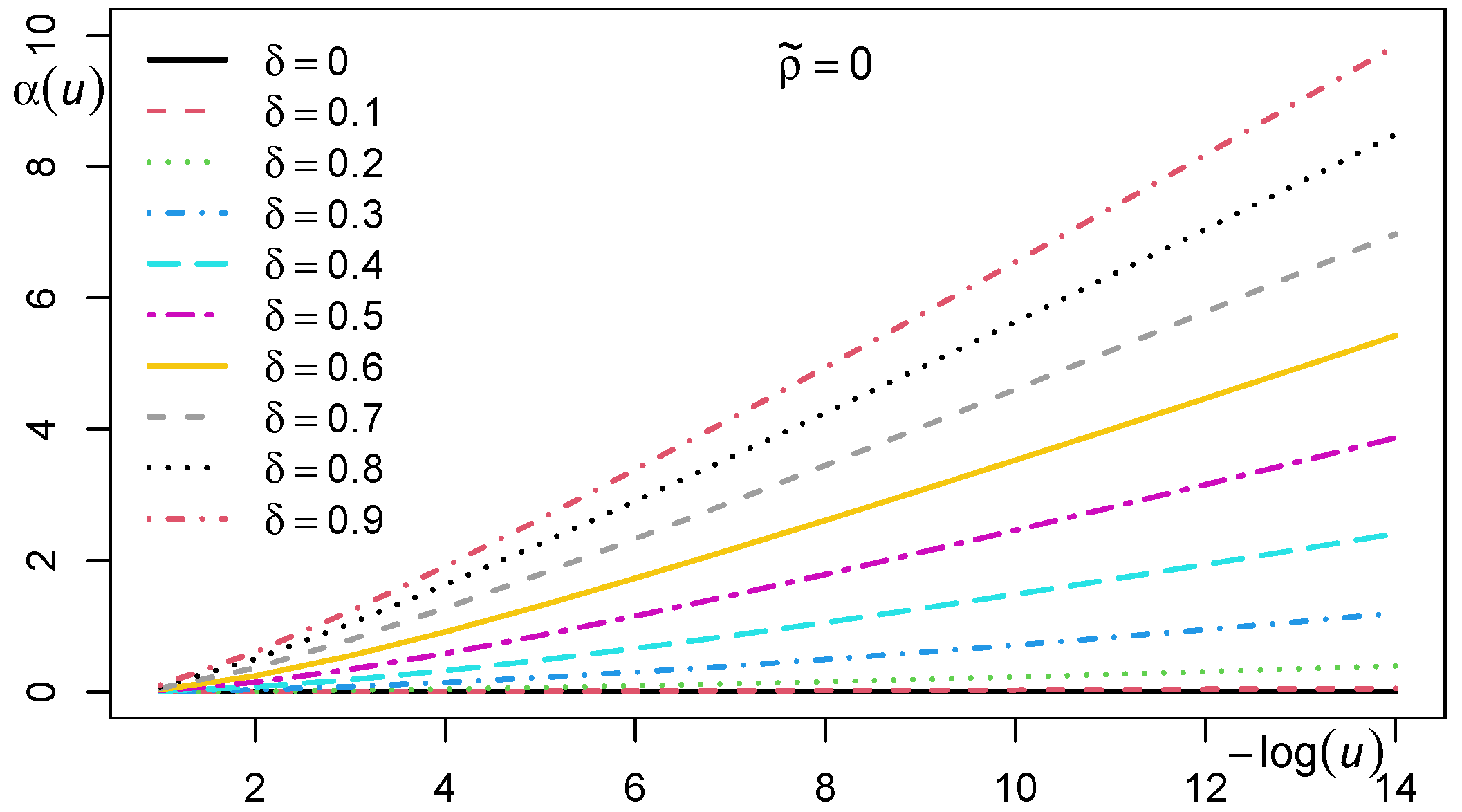
Note that ${\alpha }_{SN}(u;\delta ,\tilde{\rho })=0$ for every $u\in (0,1/2]$ if $\delta =0$. The asymptotic behavior of ${\alpha }_{SN}(u;\delta ,\tilde{\rho })$ as $u\downarrow 0$ is illustrated in Figure 3, where ${\alpha }_{SN}(u;\delta ,\tilde{\rho })$ is evaluated by (18) with the algorithm TVPACK. It is observed that the curves of ${\alpha }_{SN}(u;\delta ,\tilde{\rho })$ against $-log\left(u\right)$ are asymptotically linear.

Figure 3. The measure of tail asymmetry ${\alpha }_{SN}(u;\delta ,\tilde{\rho })$ against $-log\left(u\right)$ for different skewness parameters $\delta$ of the skew-normal copula with $\tilde{\rho }=0$.

Remark 3 

(A test of symmetry). The measure of tail asymmetry  (18) can be applied to testing symmetry of the bivariate skew-normal copula. We first note that the density of the bivariate skew-normal copula is symmetric about $\mathit{u}=(0.5,0.5)$ for $\delta =\mathbf{0}$ and not symmetric for $\delta \ne \mathbf{0}$. Then, it seems reasonable to consider a hypothesis test of symmetry of the skew-normal copula by testing the null hypothesis $H_0$: $\delta =\mathbf{0}$ against the alternative hypothesis $H_1$: $\delta \ne \mathbf{0}$.

Let ${\mathit{U}}_1,\dots ,{\mathit{U}}_n$ be a random sample from the bivariate skew-normal copula. For $u\in (0,0.5]$, the sample analogue of the measure of tail asymmetry [9] is defined by

$${\widehat{\alpha }}_{SN}\left(u\right)=log\left(\frac{T_U\left(u\right)}{T_L\left(u\right)}\right),$$

where

$$T_L\left(u\right)=\frac{1}{n}\sum _{i=1}^n\mathbf{1}(U_{1i}\le u,U_{2i}\le u),T_U\left(u\right)=\frac{1}{n}\sum _{i=1}^n\mathbf{1}(U_{1i}\ge 1-u,U_{2i}\ge 1-u),$$

${\mathit{U}}_i=(U_{1i},U_{2i})$, and $\mathbf{1}(·)$ is the indicator function, namely, $\mathbf{1}\left(A\right)=1$ if A is true and $\mathbf{1}\left(A\right)=0$ otherwise. For $0<p<1$, the $100(1-p)$% asymptotic confidence interval for ${\alpha }_{SN}(u;\mathbf{0},\tilde{\rho })$ discussed by [9] is

$$\left[{\widehat{\alpha }}_{SN}\left(u\right)-\frac{z_{p/2}\widehat{\sigma }\left(u\right)}{\sqrt{n}},{\widehat{\alpha }}_{SN}\left(u\right)+\frac{z_{p/2}\widehat{\sigma }\left(u\right)}{\sqrt{n}}\right]=:CI,$$

where $z_{p/2}={\mathsf{\Phi }}^{-1}(1-p/2)$ and $\widehat{\sigma }\left(u\right)={[\{T_L\left(u\right)+T_U\left(u\right)\}/\left\{T_L\left(u\right)T_U\left(u\right)\right\}]}^{1/2}$. Since ${\alpha }_{SN}(u;\mathbf{0},\tilde{\rho })=0$ under the null hypothesis $H_0$, the test of symmetry based on the $100(1-p)$% asymptotic confidence interval for ${\alpha }_{SN}(u;\mathbf{0},\tilde{\rho })$ is to accept $H_0$ if $\mathbf{0}\in CI$ and to reject $H_0$ if $\mathbf{0}\notin CI$. This test could be useful if analysts are interested in testing symmetry of the skew-normal copula based on observations in tails.

Figure 2 implies that, for a small u and a fixed $\tilde{\rho }$, ${\alpha }_{SN}(u;\delta ,\tilde{\rho })\ne 0$ holds for $\delta \ne 0$ and the power of this test of symmetry tends to be high for moderately large values of $\left|\delta \right|$. In particular, the test seems to be more powerful for $\tilde{\rho }\le -0.6$ than for $\tilde{\rho }>-0.6$. Figure 3 agrees with Figure 2 that, given a fixed value of u and $\tilde{\rho }=0$, the greater the value of $\delta (>0)$, the greater the power of the test. A more detailed discussion about the power of the test, including the relationship between the power and the value of u, would be future work.

Remark 4 

(Measure of tail asymmetry and TDCs). The measure of tail asymmetry (2) of the skew-normal copula can also be written by

$$\begin{array}{c}\hfill {\alpha }_{SN}(u;\delta ,\tilde{\rho })=log\left(\frac{{\lambda }_L(u;-\delta ,\tilde{\rho })}{{\lambda }_L(u;\delta ,\tilde{\rho })}\right),\end{array}$$

(21)

where

$$\begin{array}{c}\hfill {\lambda }_L(u;\delta ,\tilde{\rho })=\frac{C_{SN}(u,u;\delta ,\tilde{\rho })}{u}.\end{array}$$

(22)

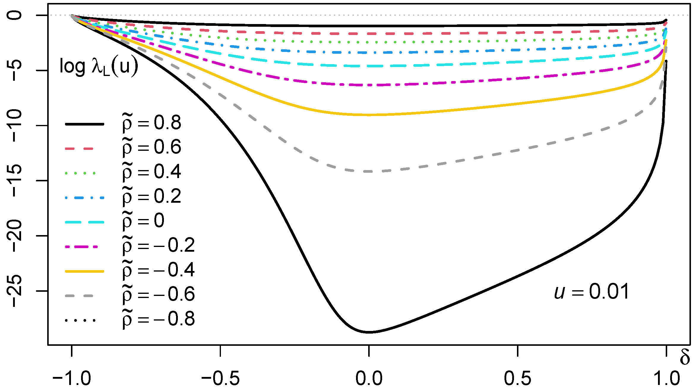
The value ${\lambda }_L(u;\delta ,\tilde{\rho })$ for a finite $u\in (0,1/2]$ can be computed by (18) with the algorithm TVPACK . Figure 4 shows the curves of $log{\lambda }_L(0.01;\delta ,\tilde{\rho })$ against δ for various correlation parameters. It is observed that ${\lambda }_L(0.01;\delta ,\tilde{\rho })$ increases as $\left|\delta \right|$ goes to 1; moreover, ${\lambda }_L(0.01;\delta ,\tilde{\rho })$ is higher for $\delta <0$ than for $\delta >0$.

Figure 4. Values of $log{\lambda }_L(u;\delta ,\tilde{\rho })$, $u=0.01$, computed by (22) with the algorithm TVPACK.

Remark 5 

(Asymptotic formulas of the TDCs). It is shown in [26] that

$$\begin{array}{c}\hfill {\lambda }_L(u;0,\rho )\sim u^{\frac{1-\rho }{1+\rho }}(1+\rho )\sqrt{\frac{1+\rho }{1-\rho }}{(-4\pi logu)}^{-\frac{\rho }{1+\rho }},u\downarrow 0.\end{array}$$

(23)

Moreover, ([14], Theorem 2) shows that, for $u\downarrow 0$,

$$\begin{array}{c}\hfill {\lambda }_L(u;\delta {\mathbf{1}}_2,\rho )\sim \left\{\begin{array}{cc}{u}^{{\beta }^2}\frac{{\left(2\pi \lambda \right)}^{{\beta }^2}}{\sqrt{\pi }\beta {(1+{\beta }^2)}^2}{(-logu)}^{{\beta }^2-\frac{1}{2}},\hfill & if\delta >0,\hfill \\ u^{\frac{1-\rho }{1+\rho }}\left(\frac{1+\rho }{2}\right)\sqrt{\frac{1+\rho }{1-\rho }}{(-\pi logu)}^{-\frac{\rho }{1+\rho }},\hfill & if\delta <0,\hfill \end{array}\right.\end{array}$$

(24)

where $\lambda =\zeta =\tilde{\alpha }(1+\rho )/\sqrt{1+{\tilde{\alpha }}^2(1-{\rho }^2)}$, $\tilde{\alpha }={\tilde{\alpha }}_1={\tilde{\alpha }}_2$, $\zeta ={\zeta }_1={\zeta }_2$ and β is defined in (A2) such that ${\beta }^2+1=2/(1+\tilde{\rho })$.

The following asymptotic formulas of ${\lambda }_L$ are also given in ([27], Appendix B) based on the tail expansion of the skew-normal copula.

$$\begin{array}{c}\hfill {\lambda }_L(u;\delta {\mathbf{1}}_2,\tilde{\rho })\sim \left\{\begin{array}{cc}{\kappa }^{-1}{u}^{\kappa -1}{(-2logu)}^{\kappa -\frac{3}{2}},\hfill & if\delta >0,\hfill \\ \left(\frac{1+\rho }{2}\right)u^{\frac{1-\rho }{1+\rho }}{(-2logu)}^{-\frac{\rho }{1+\rho }},\hfill & if\delta <0,\hfill \end{array}\right.\end{array}$$

(25)

where

$$\begin{array}{c}\hfill \kappa =\frac{2(1-{\delta }^2)}{1+\rho -2{\delta }^2}=\frac{2}{1+\tilde{\rho }}.\end{array}$$

Note that the asymptotic formulas in (25) are slightly different from those in (24), but they lead to the same tail order. With this observation, the asymptotic formulas (23), (24) and (25) yield the same limit (20) by using (21).

4. Accuracy of the Asymptotic Formulas

In Section 3, various approaches are provided to compute the measure of tail asymmetry of the skew-normal copula. It is partly observed in Figure 3 that the Formula (18) with the algorithm TVPACK gives results consistent with the asymptotic Formula (20). As mentioned in Remark 5, the measure of tail asymmetry (2) can also be computed from the asymptotic formulas (23), (24) and (25) derived in the literature. In line with this, this section explores the performance of these asymptotic formulas in a series of numerical experiments. For ease of illustration, we focus on the equiskewed case ${\delta }_1={\delta }_2=\delta$.

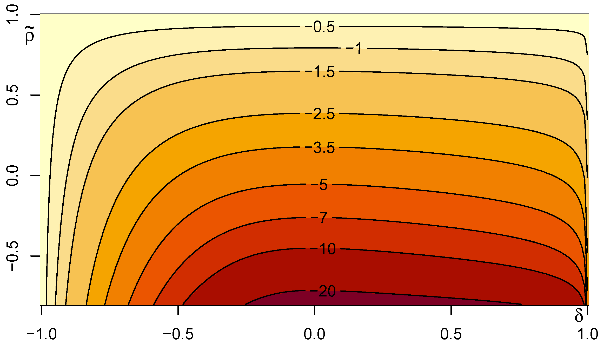
We first compute the value of ${\lambda }_L(u;\delta {\mathbf{1}}_2,\tilde{\rho })$ for $u=0.01$ as an extremely small u by (22) and (12) with ${\mathsf{\Phi }}_3$ evaluated by pmvnorm(algorithm = TVPACK) [25] in the R package mvtnorm. Figure 5 plots the contour of $log{\lambda }_L(0.01;\delta {\mathbf{1}}_2,\tilde{\rho })$ for $\delta \in [-0.999,0.999]$ and $\tilde{\rho }\in [-0.8,0.999]$ by using (12). The range of $\tilde{\rho }$ is restricted due to the numerical limitation. We observe that $log{\lambda }_L(0.01;\delta {\mathbf{1}}_2,\tilde{\rho })$ approaches 0 as $\tilde{\rho }$ and $\left|\delta \right|$ go to 1, which is consistent with the fact that the skew-normal copula is comonotonic for these parameters. Monotonicity of the function ${\lambda }_L(u;\delta {\mathbf{1}}_2,\tilde{\rho })$ with respect to $\delta$ is also indicated from Figure 5. Namely, it is observable that the value of $log{\lambda }_L(0.01;\delta {\mathbf{1}}_2,\tilde{\rho })$ for a fixed $\tilde{\rho }$ is monotonically decreasing for $\delta <0$ and increasing for $\delta >0$; thus, the minimum is attained at $\delta =0$.

Figure 5. Contour of $log{\lambda }_L(0.01;\delta {\mathbf{1}}_2,\tilde{\rho })$ for $\delta \in [-0.999,0.999]$ and $\rho \in [-0.8,0.999]$ based on (22) with the algorithm TVPACK.

For special cases, if $\rho =0$, the correlation between $Y_1$ and $Y_2$ in (1) is given by ${\delta }^2$. If $\delta =\pm 1$, the correlation is one, the variables are comonotonic, and thus $log{\lambda }_L(u;\pm {\mathbf{1}}_2,0)=log1=0$. If $\delta =0$, the variables are independent; thus, $log{\lambda }_L(u;{\mathbf{0}}_2,0)=logu$.

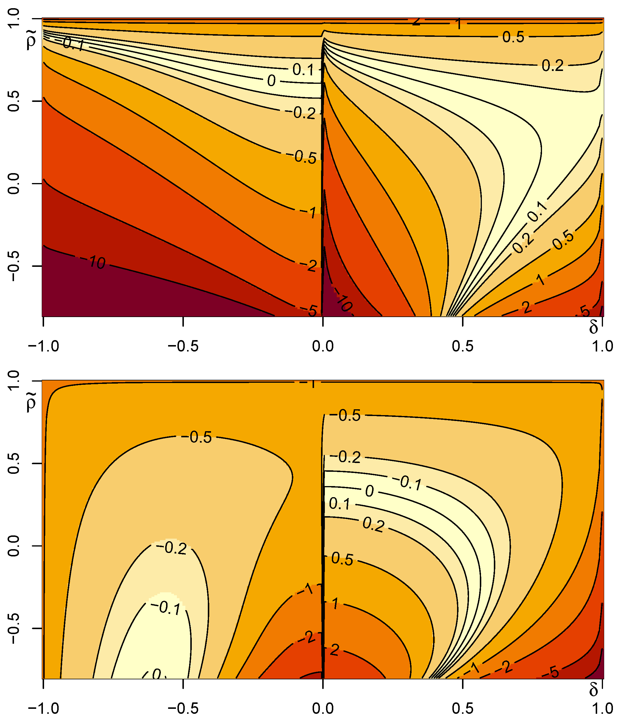
Next, we demonstrate the performance of the asymptotic formulas presented in Remark 5. Figure 6 plots the contour of the difference of $log{\lambda }_L(0.01;\delta {\mathbf{1}}_2,\tilde{\rho })$ based on the asymptotic Formula (24) and that based on the numerical evaluation of (22) with the algorithm TVPACK. The same plot is provided for the asymptotic Formula (25) instead of (24). Interestingly, we observe that the two asymptotic formulas perform well on the different areas of the parameter range. In particular, the difference of the asymptotic approximation based on the Formula (24) is large around the boundaries. Discontinuity of the asymptotic formulas is also observed around $\delta =0$, which is more visible for the Formula (24).

Figure 6. (Top) Contour of the difference of $log{\lambda }_L(0.01;\delta {\mathbf{1}}_2,\tilde{\rho })$ based on the asymptotic Formula (24) and that based on the numerical evaluation of (22) with the algorithm TVPACK for $\delta \in [-0.999,0.999]$ and $\tilde{\rho }\in [-0.8,0.999]$. (Bottom) The same contour plot based on the asymptotic Formula (25) instead of (24).

5. Conclusions

In this paper, we explored the measure of tail asymmetry proposed in [9] and its asymptotic behavior. We showed that the measure, after properly scaled, is asymptotically equivalent to the difference of the upper and lower tail orders [13]. Based on this result, we derived an analytical expression of the measure of tail asymmetry for the skew-normal copula. The performance of this formula is verified by comparing it to another analytical formula with a finite threshold. We also investigated the asymptotic formulas of the TDC of the skew-normal copula proposed in the literature. Our numerical experiments revealed that these formulas perform well for moderate values of parameters but are not recommendable for approximating the measure of tail asymmetry with finite thresholds when the parameters are at their boundaries.

Concerning future research, a simulation study and real-data analysis may be beneficial for statistical applications on the measures of tail asymmetry, particularly of the skew-normal copula. It may also be helpful to compare various measures of asymmetry for different copulas.

Appendix A.1. Parameters of the Bivariate Skew-Normal Copula

In this section, we describe detailed derivations of (15) and (17).

For the $2\times 2$ correlation matrices $\mathsf{\Omega }$ and $\mathsf{\Psi }$, let $\rho ={\mathsf{\Omega }}_{12}={\mathsf{\Omega }}_{21}$ and $\tilde{\rho }={\mathsf{\Psi }}_{12}={\mathsf{\Psi }}_{21}$. Then,

$$\rho =\mathrm{cor}\left(Y_1,Y_2\right)=\tilde{\rho }{\Delta }_1{\Delta }_2+{\delta }_1{\delta }_2,{\Delta }_1=\sqrt{1-{\delta }_1^2},{\Delta }_2=\sqrt{1-{\delta }_2^2}.$$

Here, $\tilde{\rho }$ is the partial correlation of $Y_1$ and $Y_2$ given that $Z_0$ is fixed in the trivariate random vector $\left(Z_0,Y_1,Y_2\right)$ given in (1). By using (6), we have

$$\begin{array}{c}\hfill \mathsf{\Omega }=\Delta \left(\mathsf{\Psi }+\zeta {\zeta }^{\top }\right)\Delta =\Delta \left(\left(\begin{array}{cc}1& \tilde{\rho }\\ \tilde{\rho }& 1\end{array}\right)+\left(\begin{array}{cc}{\zeta }_1^2& {\zeta }_1{\zeta }_2\\ {\zeta }_1{\zeta }_2& {\zeta }_2^2\end{array}\right)\right)\Delta ,\end{array}$$

where

$$\begin{array}{c}\hfill \Delta =\left(\begin{array}{cc}{\Delta }_1& 0\\ 0& {\Delta }_2\end{array}\right)=\left(\begin{array}{cc}\sqrt{1-{\delta }_1^2}& 0\\ 0& \sqrt{1-{\delta }_2^2}\end{array}\right)=\left(\begin{array}{cc}1/\sqrt{1+{\zeta }_1^2}& 0\\ 0& 1/\sqrt{1+{\zeta }_2^2}\end{array}\right).\end{array}$$

Hence, we have that

$$\begin{array}{cc}\hfill \mathsf{\Omega }& =\left(\begin{array}{cc}1& \rho \\ \rho & 1\end{array}\right)=\Delta \left(\begin{array}{cc}1+{\zeta }_1^2& \tilde{\rho }+{\zeta }_1{\zeta }_2\\ \tilde{\rho }+{\zeta }_1{\zeta }_2& 1+{\zeta }_2^2\end{array}\right)\Delta \hfill \\ \hfill & =\left(\begin{array}{cc}1& \frac{\tilde{\rho }+{\zeta }_1{\zeta }_2}{\sqrt{1+{\zeta }_1^2}\sqrt{1+{\zeta }_2^2}}\\ \frac{\tilde{\rho }+{\zeta }_1{\zeta }_2}{\sqrt{1+{\zeta }_1^2}\sqrt{1+{\zeta }_2^2}}& 1\end{array}\right)=\left(\begin{array}{cc}1& \tilde{\rho }{\Delta }_1{\Delta }_2+{\delta }_1{\delta }_2\\ \tilde{\rho }{\Delta }_1{\Delta }_2+{\delta }_1{\delta }_2& 1\end{array}\right),\hfill \end{array}$$

which yields (15).

Next, we check $\tilde{\alpha }$. By using

$$\begin{array}{cc}\hfill & {\mathsf{\Omega }}^{-1}\delta =\frac{1}{1-{\rho }^2}\left(\begin{array}{cc}1& -\rho \\ -\rho & 1\end{array}\right)\left(\begin{array}{c}{\delta }_1\\ {\delta }_2\end{array}\right)=\frac{1}{1-{\rho }^2}\left(\begin{array}{c}{\delta }_1-\rho {\delta }_2\\ {\delta }_2-\rho {\delta }_1\end{array}\right),\hfill \\ \hfill & 1-{\delta }^{\top }{\mathsf{\Omega }}^{-1}\delta =\frac{1-{\rho }^2-{\delta }_1^2+2\rho {\delta }_1{\delta }_2-{\delta }_2^2}{1-{\rho }^2},\hfill \end{array}$$

we have from (7) that

$$\tilde{\alpha }=\frac{{\mathsf{\Omega }}^{-1}\delta }{\sqrt{1-{\delta }^{\top }{\mathsf{\Omega }}^{-1}\delta }}=\frac{1}{\sqrt{\left(1-{\rho }^2\right)\left(1-{\rho }^2-{\delta }_1^2+2\rho {\delta }_1{\delta }_2-{\delta }_2^2\right)}}\left(\begin{array}{c}{\delta }_1-\rho {\delta }_2\\ {\delta }_2-\rho {\delta }_1\end{array}\right).$$

(A1)

Recall that the extended correlation matrix ${\mathsf{\Omega }}^{*}\left(\delta \right)$ in (10) is given by

$${\mathsf{\Omega }}^{*}\left(\delta \right)=\left(\begin{array}{ccc}1& {\delta }_1& {\delta }_2\\ {\delta }_1& 1& \rho \\ {\delta }_2& \rho & 1\end{array}\right).$$

Since

$$det{\mathsf{\Omega }}^{*}\left(\delta \right)=1-{\rho }^2-{\delta }_1^2+2\rho {\delta }_1{\delta }_2-{\delta }_2^2,$$

the parameter $\tilde{\alpha }$ in (A1) is given by

$$\tilde{\alpha }=\left(\begin{array}{c}{\tilde{\alpha }}_1\\ {\tilde{\alpha }}_2\end{array}\right)=\frac{1}{\sqrt{\left(1-{\rho }^2\right)det{\mathsf{\Omega }}^{*}\left(\delta \right)}}\left(\begin{array}{c}{\delta }_1-\rho {\delta }_2\\ {\delta }_2-\rho {\delta }_1\end{array}\right).$$

Note that this representation coincides with that in Appendix B of [27], where $({\tilde{\alpha }}_1,{\tilde{\alpha }}_2)$ and ${\mathsf{\Omega }}^{*}\left(\delta \right)$ are denoted by $({\beta }_1,{\beta }_2)$ and $\mathbf{R}$, respectively. Since

$$\begin{array}{cc}\hfill det{\mathsf{\Omega }}^{*}\left(\delta \right)=& 1-{\rho }^2-{\delta }_1^2+2\rho {\delta }_1{\delta }_2-{\delta }_2^2\hfill \\ \hfill & =1-{\left(\tilde{\rho }{\Delta }_1{\Delta }_2+{\delta }_1{\delta }_2\right)}^2-{\delta }_1^2+2\left(\tilde{\rho }{\Delta }_1{\Delta }_2+{\delta }_1{\delta }_2\right){\delta }_1{\delta }_2-{\delta }_2^2\hfill \\ \hfill & =1+{\delta }_1^2{\delta }_2^2-{\tilde{\rho }}^2\left(1-{\delta }_1^2\right)\left(1-{\delta }_2^2\right)-{\delta }_1^2-{\delta }_2^2\hfill \\ \hfill & =\left(1-{\tilde{\rho }}^2\right)\left(1-{\delta }_1^2\right)\left(1-{\delta }_2^2\right),\hfill \end{array}$$

we obtain (17).

Appendix A.2. Tail Orders of the Bivariate Skew-Normal Copula

In this section, we summarize tail orders of the bivariate skew-normal copula known in the literature. Since ${\kappa }_U(C_{SN};\delta ,\tilde{\rho })={\kappa }_L(C_{SN};-\delta ,\tilde{\rho })$, we study only the lower tail order ${\kappa }_L(C_{SN};\delta ,\tilde{\rho })$, $\tilde{\rho }\in (-1,1)$, for various $\delta =({\delta }_1,{\delta }_2)\in {(-1,1)}^2$. Moreover, we focus on the case when ${\delta }_1$ and ${\delta }_2$ have the same sign, that is, either ${\delta }_1,{\delta }_2\ge 0$ or ${\delta }_1,{\delta }_2\le 0$. In this case, we will show below that the lower tail order is summarized by (19). The interested reader is referred to [17] for more general cases of the skewness parameter. Note that the explicit forms of the tail orders of the skew-normal copula can also be found, for example, in [14,17,27]. Although they cover different cases of the parameters, their results are consistent with each other.

• Case I: δ₁ = δ₂ = δ

We first consider the equiskewed case ${\delta }_1={\delta }_2=\delta \in (-1,1)$. It follows from Theorem 2 of [14] that

$$\begin{array}{c}\hfill {\kappa }_L(C_{SN};\delta ,\tilde{\rho })=\left\{\begin{array}{cc}{\beta }^2+1,\hfill & \mathrm{if}\tilde{\alpha }>0,\hfill \\ \frac{2}{1+\rho },\hfill & \mathrm{if}\tilde{\alpha }<0,\hfill \end{array}\right.\end{array}$$

where

$$\begin{array}{c}\hfill \tilde{\alpha }=\frac{\delta }{\sqrt{(1+\tilde{\rho })(1+\rho )(1-{\delta }^2)}},\end{array}$$

and

$$\begin{array}{c}\hfill \beta =\sqrt{\frac{(1-\rho )(1+2(1+\rho ){\tilde{\alpha }}^2)}{1+\rho }},\end{array}$$

(A2)

and thus, by calculation,

$$\begin{array}{c}\hfill {\beta }^2+1=\frac{1-\tilde{\rho }}{1+\tilde{\rho }}+1=\frac{2}{1+\tilde{\rho }}.\end{array}$$

Note that the signs of $\tilde{\alpha }$ and $\delta$ are identical, and that $\delta =0$ if and only if $\tilde{\alpha }=0$. When $\delta =0$, we have that

$$\begin{array}{c}\hfill {\kappa }_L(C_{SN};\mathbf{0},\tilde{\rho })=\frac{2}{1+\tilde{\rho }}=\frac{2}{1+\rho };\end{array}$$

see also Appendix B of [27].

• Case III: δ₁, δ₂ < 0

It is shown in [17] that

$${\kappa }_L\left(C_{\mathrm{SN}};\delta ,\tilde{\rho }\right)=\frac{2}{1+\rho },$$

which is also derived in [27]. Note that the condition ${\Delta }_1{\tilde{\alpha }}_1+{\Delta }_2{\tilde{\alpha }}_2<0$ is imposed in [27], and this condition is implied by (16). Indeed, we have from (17) that

$${\Delta }_1{\tilde{\alpha }}_1+{\Delta }_2{\tilde{\alpha }}_2=\frac{{\Delta }_1\left({\delta }_1-\rho {\delta }_2\right)+{\Delta }_2\left({\delta }_2-\rho {\delta }_1\right)}{\sqrt{\left(1-{\rho }^2\right)det{\mathsf{\Omega }}^{*}\left(\delta \right)}},$$

(A3)

and thus the sign of ${\Delta }_1{\tilde{\alpha }}_1+{\Delta }_2{\tilde{\alpha }}_2$ equals to that of the numerator of the right-hand side of (A3). From (16), the inequality ${\Delta }_1{\delta }_2+{\Delta }_2{\delta }_1<0$ implies that

$$\begin{array}{cc}\hfill & {\Delta }_1\left({\delta }_1-\rho {\delta }_2\right)+{\Delta }_2\left({\delta }_2-\rho {\delta }_1\right)={\Delta }_1{\delta }_1+{\Delta }_2{\delta }_2-\rho \left({\Delta }_1{\delta }_2+{\Delta }_2{\delta }_1\right)\hfill \\ \hfill & <{\Delta }_1{\delta }_1+{\Delta }_2{\delta }_2-\left({\delta }_1{\delta }_2+{\Delta }_1{\Delta }_2\right)\left({\Delta }_1{\delta }_2+{\Delta }_2{\delta }_1\right)\hfill \\ \hfill & ={\Delta }_1{\delta }_1+{\Delta }_2{\delta }_2-{\Delta }_1{\delta }_1{\delta }_2^2-{\Delta }_2{\delta }_1^2{\delta }_2-{\Delta }_2\left({1-\delta }_1^2\right){\delta }_2-{\Delta }_1\left({1-\delta }_2^2\right){\delta }_1=0,\hfill \end{array}$$

and thus ${\Delta }_1{\tilde{\alpha }}_1+{\Delta }_2{\tilde{\alpha }}_2<0$.

• Case II: δ₁, δ₂ < 0

It is shown in [17] that

$$\begin{array}{cc}\hfill & {\kappa }_L\left(C_{\mathrm{SN}}:\delta ,\tilde{\rho }\right)={\kappa }_U\left(C_{\mathrm{SN}}:-\delta ,\tilde{\rho }\right)\hfill \\ \hfill & =\frac{1}{1-{\rho }^2}\left\{\frac{1+{\tilde{\alpha }}_1^2\left(1-{\rho }^2\right)}{1+{\zeta }_1^2}+\frac{1+{\tilde{\alpha }}_2^2\left(1-{\rho }^2\right)}{1+{\zeta }_2^2}+\frac{2\left({\tilde{\alpha }}_1{\tilde{\alpha }}_2\left(1-{\rho }^2\right)-\rho \right)}{\sqrt{\left(1+{\zeta }_1^2\right)\left(1+{\zeta }_2^2\right)}}\right\}\hfill \\ \hfill & =\frac{1}{1-{\rho }^2}\left\{\frac{1}{1+{\zeta }_1^2}+\frac{1}{1+{\zeta }_2^2}-\frac{2\rho }{\sqrt{\left(1+{\zeta }_1^2\right)\left(1+{\zeta }_2^2\right)}}\right.\hfill \\ \hfill & \left.+\left(1-{\rho }^2\right){\left(\frac{{\tilde{\alpha }}_1}{\sqrt{1+{\zeta }_1^2}}+\frac{{\tilde{\alpha }}_2}{\sqrt{1+{\zeta }_2^2}}\right)}^2\right\}\hfill \\ \hfill & =\frac{{\Delta }_1^2+{\Delta }_2^2-2\rho {\Delta }_1{\Delta }_2}{1-{\rho }^2}+{\left({\Delta }_1{\tilde{\alpha }}_1+{\Delta }_2{\tilde{\alpha }}_2\right)}^2.\hfill \end{array}$$

(A4)

Note that, in [17], ${\zeta }_1$ and ${\zeta }_2$ above are denoted by ${\lambda }_1$ and ${\lambda }_2$, respectively. The Formula (A4) is also derived in Appendix B of [27]. Note again that the condition ${\Delta }_1{\tilde{\alpha }}_1+{\Delta }_2{\tilde{\alpha }}_2>0$ imposed in [27] is implied by (16). We will check that

$$\begin{array}{c}\hfill \frac{{\Delta }_1^2+{\Delta }_2^2-2\rho {\Delta }_1{\Delta }_2}{1-{\rho }^2}+{\left({\Delta }_1{\tilde{\alpha }}_1+{\Delta }_2{\tilde{\alpha }}_2\right)}^2=\frac{2}{1+\tilde{\rho }},\end{array}$$

(A5)

that is, the expression (A4) can be simplified as

$${\kappa }_L\left(C_{\mathrm{SN}}:\delta ,\tilde{\rho }\right)={\kappa }_U\left(C_{\mathrm{SN}}:-\delta ,\tilde{\rho }\right)=\frac{2}{1+\tilde{\rho }}.$$

First, by multiplying $\left(1-{\rho }^2\right)$ on the right-hand side of (A5), the desired equation is equivalent to

$${\Delta }_1^2+{\Delta }_2^2-2\rho {\Delta }_1{\Delta }_2+\left(1-{\rho }^2\right){\left({\Delta }_1{\tilde{\alpha }}_1+{\Delta }_2{\tilde{\alpha }}_2\right)}^2=\frac{2\left(1-\tilde{\rho }\right)\left(1-{\rho }^2\right)}{\left(1-{\tilde{\rho }}^2\right)},$$

which is also equivalent to

$$\begin{array}{cc}\hfill & (1-{\tilde{\rho }}^2){\Delta }_1^2{\Delta }_2^2\left\{{\Delta }_1^2+{\Delta }_2^2-2\rho {\Delta }_1{\Delta }_2+\left(1-{\rho }^2\right){\left({\Delta }_1{\tilde{\alpha }}_1+{\Delta }_2{\tilde{\alpha }}_2\right)}^2\right\}=2\left(1-\tilde{\rho }\right)\left(1-{\rho }^2\right){\Delta }_1^2{\Delta }_2^2\hfill \end{array}$$

(A6)

by multiplying $\left(1-{\tilde{\rho }}^2\right){\Delta }_1^2{\Delta }_2^2$ on both sides. Since

$${\left({\Delta }_1{\tilde{\alpha }}_1+{\Delta }_2{\tilde{\alpha }}_2\right)}^2=\frac{{\left\{\left({\delta }_1-\rho {\delta }_2\right){\Delta }_1+\left({\delta }_2-\rho {\delta }_1\right){\Delta }_2\right\}}^2}{\left(1-{\rho }^2\right)\left(1-{\tilde{\rho }}^2\right)\left(1-{\delta }_1^2\right)\left(1-{\delta }_2^2\right)},$$

the left-hand side of (A6) reduces to

$$\begin{array}{c}\hfill (1-{\tilde{\rho }}^2){\Delta }_1^2{\Delta }_2^2({\Delta }_1^2+{\Delta }_2^2)-2\rho (1-{\tilde{\rho }}^2){\Delta }_1^3{\Delta }_2^3+{\left\{\left({\delta }_1-\rho {\delta }_2\right){\Delta }_1+\left({\delta }_2-\rho {\delta }_1\right){\Delta }_2\right\}}^2.\end{array}$$

(A7)

The last two terms of (A7) are expanded into

$$\begin{array}{cc}\hfill -2\rho \left(1-{\tilde{\rho }}^2\right){\Delta }_1^3{\Delta }_2^3& +{\left\{\left({\delta }_1-\rho {\delta }_2\right){\Delta }_1+\left({\delta }_2-\rho {\delta }_1\right){\Delta }_2\right\}}^2\hfill \\ \hfill & =-2\rho \left(1-{\tilde{\rho }}^2\right){\Delta }_1^3{\Delta }_2^3+2\left({\delta }_1-\rho {\delta }_2\right)\left({\delta }_2-\rho {\delta }_1\right){\Delta }_1{\Delta }_2\hfill \\ \hfill & +{\left({\delta }_1-\rho {\delta }_2\right)}^2{\Delta }_1^2+{\left({\delta }_2-\rho {\delta }_1\right)}^2{\Delta }_2^2.\hfill \end{array}$$

(A8)

By using ${\delta }_1{\delta }_2-\rho =-\tilde{\rho }{\Delta }_1{\Delta }_2$, the coefficient of ${\Delta }_1{\Delta }_2$ at the first two terms in the right-hand side of (A8) is given by

$$\begin{array}{cc}\hfill & -2\rho \left(1-{\tilde{\rho }}^2\right)\left(1-{\delta }_1^2\right)\left(1-{\delta }_2^2\right)+2\left({\delta }_1-\rho {\delta }_2\right)\left({\delta }_2-\rho {\delta }_1\right)\hfill \\ \hfill & =-2\rho \left(1-{\delta }_1^2-{\delta }_2^2+{\delta }_1^2{\delta }_2^2\right)+2\rho {\tilde{\rho }}^2\left(1-{\delta }_1^2\right)\left(1-{\delta }_2^2\right)+2\left({\delta }_1{\delta }_2-\rho {\delta }_1^2-\rho {\delta }_2^2+{\rho }^2{\delta }_1{\delta }_2\right)\hfill \\ \hfill & =2\left({\delta }_1{\delta }_2-\rho -\rho {\delta }_1^2{\delta }_2^2+{\rho }^2{\delta }_1{\delta }_2\right)+2\rho {\tilde{\rho }}^2\left(1-{\delta }_1^2\right)\left(1-{\delta }_2^2\right)\hfill \\ \hfill & =-2\tilde{\rho }\left(1-\rho {\delta }_1{\delta }_2\right){\Delta }_1{\Delta }_2+2\rho {\tilde{\rho }}^2{\Delta }_1^2{\Delta }_2^2\hfill \\ \hfill & =-2\tilde{\rho }\left(1-\rho {\delta }_1{\delta }_2-\rho \tilde{\rho }{\Delta }_1{\Delta }_2\right){\Delta }_1{\Delta }_2\hfill \\ \hfill & =-2\tilde{\rho }\left(1-{\rho }^2\right){\Delta }_1{\Delta }_2.\hfill \end{array}$$

(A9)

By using $\rho =\tilde{\rho }{\Delta }_1{\Delta }_2+{\delta }_1{\delta }_2$, the last two terms of the right-hand side of (A8) are rearranged as follows:

$$\begin{array}{cc}\hfill & {\left({\delta }_1-\rho {\delta }_2\right)}^2{\Delta }_1^2+{\left({\delta }_2-\rho {\delta }_1\right)}^2{\Delta }_2^2\hfill \\ \hfill & ={\left({\delta }_1\left(1-{\delta }_2^2\right)-\tilde{\rho }{\Delta }_1{\Delta }_2{\delta }_2\right)}^2{\Delta }_1^2+{\left({\delta }_2\left(1-{\delta }_1^2\right)-\tilde{\rho }{\Delta }_1{\Delta }_2{\delta }_1\right)}^2{\Delta }_2^2\hfill \\ \hfill & =\left\{{({\delta }_1{\Delta }_2-\tilde{\rho }{\Delta }_1{\delta }_2)}^2+{({\delta }_2{\Delta }_1-\tilde{\rho }{\Delta }_2{\delta }_1)}^2\right\}{\Delta }_1^2{\Delta }_2^2\hfill \\ \hfill & =\left\{\left({\delta }_1^2+{\delta }_2^2-2{\delta }_1^2{\delta }_2^2\right)\left(1+{\tilde{\rho }}^2\right)-4\tilde{\rho }{\delta }_1{\delta }_2{\Delta }_1{\Delta }_2\right\}{\Delta }_1^2{\Delta }_2^2.\hfill \end{array}$$

(A10)

Combining (A9) and (A10), the term (A8) reduces to

$$\begin{array}{cc}\hfill -2\rho & \left(1-{\tilde{\rho }}^2\right){\Delta }_1^3{\Delta }_2^3+{\left\{\left({\delta }_1-\rho {\delta }_2\right){\Delta }_1+\left({\delta }_2-\rho {\delta }_1\right){\Delta }_2\right\}}^2\hfill \\ \hfill & =\left\{-2\tilde{\rho }\left(1-{\rho }^2\right)+\left({\delta }_1^2+{\delta }_2^2-2{\delta }_1^2{\delta }_2^2\right)\left(1+{\tilde{\rho }}^2\right)-4\tilde{\rho }{\delta }_1{\delta }_2{\Delta }_1{\Delta }_2\right\}{\Delta }_1^2{\Delta }_2^2.\hfill \end{array}$$

Therefore, the desired equation (A6) is now

$$\begin{array}{c}\hfill (1-{\tilde{\rho }}^2)\left\{{\Delta }_1^2+{\Delta }_2^2-2\rho {\Delta }_1{\Delta }_2+\left(1-{\rho }^2\right){\left({\Delta }_1{\tilde{\alpha }}_1+{\Delta }_2{\tilde{\alpha }}_2\right)}^2\right\}=2\left(1-\tilde{\rho }\right)\left(1-{\rho }^2\right),\end{array}$$

which can be checked as follows:

$$\begin{array}{cc}\hfill & (1-{\tilde{\rho }}^2)\left\{{\Delta }_1^2+{\Delta }_2^2-2\rho {\Delta }_1{\Delta }_2+\left(1-{\rho }^2\right){\left({\Delta }_1{\tilde{\alpha }}_1+{\Delta }_2{\tilde{\alpha }}_2\right)}^2\right\}\hfill \\ \hfill & =\left(2-{\delta }_1^2-{\delta }_2^2\right)\left(1-{\tilde{\rho }}^2\right)-2\tilde{\rho }\left(1-{\rho }^2\right)+\left({\delta }_1^2+{\delta }_2^2-2{\delta }_1^2{\delta }_2^2\right)\left(1+{\tilde{\rho }}^2\right)-4\tilde{\rho }{\delta }_1{\delta }_2{\Delta }_1{\Delta }_2\hfill \\ \hfill & =2\left(1-{\delta }_1^2{\delta }_2^2-{\tilde{\rho }}^2{\Delta }_1^2{\Delta }_2^2-2\tilde{\rho }{\delta }_1{\delta }_2{\Delta }_1{\Delta }_2\right)-2\tilde{\rho }\left(1-{\rho }^2\right)\hfill \\ \hfill & =2(1-{\rho }^2)-2\tilde{\rho }(1-{\rho }^2)\hfill \\ \hfill & =2\left(1-\tilde{\rho }\right)\left(1-{\rho }^2\right).\hfill \end{array}$$

• Case IV: One of δ₁ and δ₂ Is Zero and the Other Is Negative

By symmetry, it suffices to consider the case when ${\delta }_1=0$ and ${\delta }_2<0$. In this case, [17] shows that ${\kappa }_L\left(C_{\mathrm{SN}}:\delta ,\tilde{\rho }\right)=2/(1+\rho )$.

• Case V: One of δ₁ and δ₂ Is Zero and the Other Is Positive

By symmetry, it suffices to consider the case when ${\delta }_1=0$ and ${\delta }_2>0$. In this case, [17] shows that, if ${\tilde{\alpha }}_1+{\tilde{\alpha }}_2{\Delta }_2>0$, then

$$\begin{array}{c}\hfill {\kappa }_L\left(C_{\mathrm{SN}}:\delta ,\tilde{\rho }\right)=\frac{{({\Delta }_2-\rho )}^2}{(1-{\rho }^2)}+{({\tilde{\alpha }}_1+{\tilde{\alpha }}_2{\Delta }_2)}^2+1.\end{array}$$

The condition ${\tilde{\alpha }}_1+{\tilde{\alpha }}_2{\Delta }_2>0$ is always satisfied since

$$\begin{array}{c}\hfill {\tilde{\alpha }}_1+{\tilde{\alpha }}_2{\Delta }_2=\frac{{\delta }_2({\Delta }_2-\rho )}{\sqrt{(1-{\rho }^2)det{\mathsf{\Omega }}^{*}\left(\delta \right)}}\end{array}$$

and $\rho <{\Delta }_2$ by (16). Since $det{\mathsf{\Omega }}^{*}\left(\delta \right)=(1-{\tilde{\rho }}^2)(1-{\delta }_2^2)$ and $\rho =\tilde{\rho }{\Delta }_2$, we have that

$$\begin{array}{cc}\hfill \frac{{({\Delta }_2-\rho )}^2}{(1-{\rho }^2)}+{({\tilde{\alpha }}_1+{\tilde{\alpha }}_2{\Delta }_2)}^2& =\frac{{({\Delta }_2-\rho )}^2\{{\delta }_2^2+det{\mathsf{\Omega }}^{*}\left(\delta \right)\}}{(1-{\rho }^2)det{\mathsf{\Omega }}^{*}\left(\delta \right)}\hfill \\ \hfill & =\frac{{(1-\tilde{\rho })}^2(1-{\tilde{\rho }}^2+{\tilde{\rho }}^2{\delta }_2^2)}{(1-{\rho }^2)(1-{\tilde{\rho }}^2)}\hfill \\ \hfill & =\frac{(1-\tilde{\rho })(1-{\tilde{\rho }}^2(1-{\delta }_2^2))}{(1-{\rho }^2)(1+\tilde{\rho })}\hfill \\ \hfill & =\frac{1-\tilde{\rho }}{1+\tilde{\rho }}.\hfill \end{array}$$

Therefore,

$$\begin{array}{c}\hfill {\kappa }_L\left(C_{\mathrm{SN}}:\delta ,\tilde{\rho }\right)=\frac{{({\Delta }_2-\rho )}^2}{(1-{\rho }^2)}+{({\tilde{\alpha }}_1+{\tilde{\alpha }}_2{\Delta }_2)}^2+1=\frac{2}{1+\tilde{\rho }}.\end{array}$$

References

1. Ang, A.; Chen, J. Asymmetric correlations of equity portfolios. J. Financ. Econ. 2002, 63, 443–494. [Google Scholar] [CrossRef]
2. Azzalini, A. The Skew-Normal and Related Families; Cambridge University Press: Cambridge, UK, 2014. [Google Scholar] [CrossRef]
3. Azzalini, A.; Dalla Valle, A. The multivariate skew-normal distribution. Biometrika 1996, 83, 715–726. [Google Scholar] [CrossRef]
4. Azzalini, A.; Capitanio, A. Distributions generated by perturbation of symmetry with emphasis on a multivariate skew t-distribution. J. R. Stat. Soc. Ser. B 2003, 65, 367–389. [Google Scholar] [CrossRef]
5. Nikoloulopoulos, A.K.; Joe, H.; Li, H. Vine copulas with asymmetric tail dependence and applications to financial return data. Comput. Stat. Data Anal. 2012, 56, 3659–3673. [Google Scholar] [CrossRef]
6. Dobric, J.; Frahm, G.; Schmid, F. Dependence of Stock Returns in Bull and Bear Markets. Depend. Model. 2013, 1, 94–110. [Google Scholar] [CrossRef]
7. Rosco, J.; Joe, H. Measures of tail asymmetry for bivariate copulas. Stat. Pap. 2013, 54, 709–726. [Google Scholar] [CrossRef]
8. Krupskii, P. Copula-based measures of reflection and permutation asymmetry and statistical tests. Stat. Pap. 2017, 58, 1165–1187. [Google Scholar] [CrossRef]
9. Kato, S.; Yoshiba, T.; Eguchi, S. Copula-based measures of asymmetry between the lower and upper tail probabilities. Stat. Pap. 2022, 63, 1907–1929. [Google Scholar] [CrossRef]
10. Azzalini, A.; Capitanio, A. Statistical applications of the multivariate skew normal distribution. J. R. Stat. Soc. Ser. (Stat. Methodol.) 1999, 61, 579–602. [Google Scholar] [CrossRef]
11. Adcock, C.; Azzalini, A. A selective overview of skew-elliptical and related distributions and of their applications. Symmetry 2020, 12, 118. [Google Scholar] [CrossRef] [Green Version]
12. Azzalini, A. An overview on the progeny of the skew-normal family—A personal perspective. J. Multivar. Anal. 2022, 188, 104851. [Google Scholar] [CrossRef]
13. Hua, L.; Joe, H. Tail order and intermediate tail dependence of multivariate copulas. J. Multivar. Anal. 2011, 102, 1454–1471. [Google Scholar] [CrossRef] [Green Version]
14. Fung, T.; Seneta, E. Tail asymptotics for the bivariate skew normal. J. Multivar. Anal. 2016, 144, 129–138. [Google Scholar] [CrossRef]
15. Sibuya, M. Bivariate extreme statistics, I. Ann. Inst. Stat. Math. 1960, 11, 195–210. [Google Scholar] [CrossRef]
16. Joe, H. Parametric Families of Multivariate Distributions with Given Margins. J. Multivar. Anal. 1993, 46, 262–282. [Google Scholar] [CrossRef] [Green Version]
17. Fung, T.; Seneta, E. Tail asymptotics for the bivariate skew normal in the general case. arXiv 2022, arXiv:2210.01284. [Google Scholar]
18. Lao, X.; Peng, Z.; Nadarajah, S. Tail Dependence Functions of Two Classes of Bivariate Skew Distributions. Methodol. Comput. Appl. Probab. 2023, 25, 10. [Google Scholar] [CrossRef]
19. Fung, T.; Seneta, E. Tail dependence for two skew t distributions. Stat. Probab. Lett. 2010, 80, 784–791. [Google Scholar] [CrossRef]
20. Fung, T.; Seneta, E. Tail dependence and skew distributions. Quant. Financ. 2011, 11, 327–333. [Google Scholar] [CrossRef]
21. Fung, T.; Seneta, E. Convergence rate to a lower tail dependence coefficient of a skew-t distribution. J. Multivar. Anal. 2014, 128, 62–72. [Google Scholar] [CrossRef]
22. Ling, C.; Peng, Z. Tail dependence for two skew slash distributions. Stat. Interfaces 2015, 8, 63–69. [Google Scholar] [CrossRef]
23. Tian, W.; Li, H.; Gupta, A.K. Tail Dependence of Generalized Modified Skew Slash Distribution. J. Stat. Theory Pract. 2022, 16, 4. [Google Scholar] [CrossRef]
24. Ning, J.; Yi, W. Tail dependence for skew Laplace distribution and skew Cauchy distribution. Commun. Stat. Theory Methods 2016, 45, 5224–5233. [Google Scholar] [CrossRef]
25. Genz, A. Numerical computation of rectangular bivariate and trivariate normal and t probabilities. Stat. Comput. 2004, 14, 251–260. [Google Scholar] [CrossRef]
26. Coles, S.; Heffernan, J.; Tawn, J. Dependence measures for extreme value analyses. Extremes 1999, 2, 339–365. [Google Scholar] [CrossRef]
27. Li, X.; Joe, H. Estimation of multivariate tail quantities. Comput. Stat. Data Anal. 2023, 185, 107761. [Google Scholar] [CrossRef]
28. Nelsen, R.B. An Introduction to Copulas; Springer: New York, NY, USA, 2006. [Google Scholar] [CrossRef]
29. Resnick, S.I. Heavy-Tail Phenomena: Probabilistic and Statistical Modeling; Springer Series in Operations Research and Financial Engineering; Springer: New York, NY, USA, 2007. [Google Scholar] [CrossRef]