Review

Prediction Intervals: A Geometric View

by
Evgeny Nikulchev
1,* and
Alexander Chervyakov
2
1
Department of Digital Data Processing Technologies, MIREA—Russian Technological University, Moscow 119454, Russia
2
Federal Treasury, Ministry of Finance of the Russian Federation, Moscow 101000, Russia
*
Author to whom correspondence should be addressed.
Symmetry 2023, 15(4), 781; https://doi.org/10.3390/sym15040781
Submission received: 13 February 2023 / Revised: 15 March 2023 / Accepted: 21 March 2023 / Published: 23 March 2023
(This article belongs to the Special Issue Recent Advances in the Application of Symmetry Group)

Abstract

:
This article provides a review of the approaches to the construction of prediction intervals. To increase the reliability of prediction, point prediction methods are replaced by intervals for many aims. The interval prediction generates a pair as future values, including the upper and lower bounds for each prediction point. That is, according to historical data, which include a graph of a continuous and discrete function, two functions will be obtained as a prediction, i.e., the upper and lower bounds of estimation. In this case, the prediction boundaries should provide guaranteed probability of the location of the true values inside the boundaries found. The task of building a model from a time series is, by its very nature, incorrect. This means that there is an infinite set of equations whose solution is close to the time series for machine learning. In the case of interval use, the inverse problem of dynamics allows us to choose from the entire range of modeling methods, using confidence intervals as solutions, or intervals of a given width, or those chosen as a solution to the problems of multi-criteria optimization of the criteria for evaluating interval solutions. This article considers a geometric view of the prediction intervals and a new approach is given.

1. Introduction

A dynamic system is defined as a model of the evolution of a process, the state of which is determined based on the initial state and the equations of dynamics. The tasks involved in predicting or obtaining numerical estimates of the future values of the observed process based on historical data include the process of determining a discrete dynamic system whose behavior would correspond to real data (perhaps obtaining a continuous model, a decision that is decreed in time intervals that correspond to the relevant changes—the real process). From the point of view of geometry, the graph that corresponds to the solution should differ as little as possible from the graph that corresponds to the observed process, that is, there is a transformation close to unity, under conditions of an insignificant change in symmetry.
Modern methods for building predictive models [1,2], based on machine learning, including artificial intelligence methods [3,4], aim to find the most suitable systems that minimize the deviation of the observed time series from the model graph (solution of the equation of evolution of a dynamic system), which requires achieving a given accuracy or qualitative adequacy of the phase trajectories. From the point of view of geometry, we must eliminate the violation of symmetry.
For a dynamic system, the concepts of robust models stand in opposition to sensitivity [5], while, as a rule, a robust model is defined as insensitive in its dynamic behavior and dynamic and frequency characteristics when the model parameters change (which can be called parametric robustness). As opposed to interval parameter assignments, one can introduce dynamic output robustness, i.e., the solution determined by a dynamic system with fixed parameters has an interval form, known as prediction intervals (PI).
Predictions that are not in point form, but in the form of ranges of values, are called forecast intervals (PI). However, this involves not only forecasting, but also interval extrapolation from point historical data. It seems appropriate to call such a model a robust model, with robust output. Thus, in the problem of building a model according to a time series, i.e., an ill-posed problem (the inverse problem of dynamics), robust interval models can be understood as dynamic systems, the solution of which is given by values at intervals, while the interval is reliable and adequately includes the original time series and gives a reliable prediction. Under these conditions, several (completely different) models can determine the initial interval around the observed states of the system.
In other words, for the time series { X ( t ) , ( t = 0 , 1 , 2 , ) }, the following functions are defined f i ( x ( t ) ) = y ( t + 1 ) [ y ;     y + ] i , where f i represents various analytic functions, or functional expansions; t represents discrete time (point number); x ( t ) is the value of the state of the system at the moment t; y is the computed value; y , y + are the lower and upper limits of the interval, respectively; I is the function number. The interval can be defined as a confidence interval in a stochastic model and it can be based on interval estimates with measurement errors, or it can be fixed and set based on the conditions of the problem, and the value of the interval can be the result of solving a variational or optimization issue of the given criteria presented in intervals.
Thus, it is possible to define a new class of systems dynamic models (stochastic or deterministic), the parameters of which are functions without uncertainties, and the solution is an interval form. Here, we also consider the transformation of a plot of a function into an interval. In addition, the operation of the idempotent addition of intervals is introduced, which transforms the set of graphs into a semiring. One can recall that if we consider particular solutions of (evolutionary) differential equations, they form Lie groups (a symmetry group). This paper considers PI from geometric positions. When using PI for a group of interconnected series, for example, a portfolio of financial instruments, forecasting the energy consumption of a group or other structurally complex dynamic objects [6] allows us to reduce the requirements for the width of forecasts, paying attention to any other characteristics, for example, absenteeism forecast values beyond the lower limit of the forecast.
The contribution of this article is presented in the following list:
-
A geometric approach for interval forecasts is proposed;
-
A review of PI methods based on a geometric view was carried out;
-
A new approach to the construction of robust output models is proposed.
In this article, we review and construct new types of models. The structure of the article is as follows: Section 2, a review of PIs is carried out, in Section 3, a selection of criteria for evaluating interval solutions is presented, in Section 4, a new theory of interval models is proposed, and an example of construction is given. Section 5 contains the conclusion.

2. Prediction Intervals: Review

The task of prediction is the task of finding the values of the observed process in the future for the number of reports (for discrete systems and time series) or a time interval (for continuous systems) called the forecast horizon. In terms of geometry, it is required to extend or extrapolate the graph (continuous or discrete) by a given value. Traditional time series methods look for the next point at the next point in time, provided the current and historical data are known. Unlike the point prediction, the prediction interval (PI) provides the numerical value of the range in which the system will be at the next point in time. At the same time, the graph itself (initial data) is the same as for the point prediction. In other words, for a function graph (time series), the prediction will be an interval characterized by upper and lower boundaries. It is often argued that the PI is the most probable interval of values, but this is not entirely true, as it all depends on the conditions for the width of the interval.
With the use of PIs, there is a blurring of the accuracy of the prediction, but at the same time, the degree of uncertainty is reduced, and ensures the robustness of the model in terms of output. A guaranteed hit in each prediction interval is a reduction in the error, with a sufficiently wide interval and a complete elimination of the error. Based on historical data (time interval) in the form of a graph, the prediction includes two non-intersecting graphs for a given forecast interval; the first graph is the upper limit, while the lower graph is the lower forecast limit. We are looking for two transformations—the original chart into the chart of the upper boundary and the chart of the lower boundary. In the resulting range, an infinite number of functions can be included, including those corresponding to real data.
Currently, PIs, as the most intuitive approach, have attracted a significant amount of attention [7,8,9,10]. This approach is intuitive, since a weather forecast is usually a range of predicted temperatures for each moment of time or each day. The methods are widely used both for weather data, wind forecasting [7], in energy [8] and in other applied areas [9,10]. The generality of application can be characterized as follows: (1) the problem has pronounced trends and seasonal components; (2) there are portfolios of several signals; (3) for forecasts, there are requirements for reliable upper or lower bounds.
In recent years, probabilistic prediction methods have been extensively studied to effectively quantify uncertainties. A probabilistic prediction generates probability density functions [11], quantiles [12], or intervals [13] in applied prediction problems. Traditional interval prediction methods include fuzzy inference [14], beta distribution function [15] and Gaussian processes, autoregressive integrated moving average models and log-normal processes for obtaining probabilistic predictions [16,17,18]. The features of such solutions are the assumptions about the type of distribution, while Gaussian processes require significant computational resources to estimate the covariance matrices [19]. Numerical methods for obtaining quasi-Gaussian noise can obtain negative values of the interval, which is inconsistent with the physical meaning of the problem. For short-term prediction, the following were proposed: a combination of a kernel-based support vector quantile regression model and Copula theory [20]; the use of Yeo–Johnson transformation quantile regression and Gaussian kernel function [21]; machine learning methods, which are now widely used [22,23]. In these papers, the results were evaluated based on the PI coverage probability and the normalized mean PI width. The features of the methods are high mathematical computational complexity, with the need to identify seasonal components.
As a non-parametric method, the proposed lower and upper bound estimation (LUBE) [24,25] can effectively solve the above problem by constructing the PI directly from the input data, without any additional assumptions about the distribution of the data. The LUBE method was proposed in [26] and is aimed at constructing narrow PIs with a high probability. In general, LUBE can be solved in single-purpose and multi-purpose frameworks. For example, in [27], a single-target structure for LUBE is proposed in which the average PI width is minimized with restrictions. In [28], it was proposed to decompose and group the series into different components using the empirical mode and sample decomposition methods. In a multi-criteria framework [29], the coverage probability and the average PI width are simultaneously optimized to obtain a set of Pareto-optimal solutions. Here, partial decomposition and smoothing of fluctuations in wind power series were used to correctly preprocess data for the forecast model. As a rule, multicriteria involve building a compromise between the maximum probability of real values falling into the found interval and obtaining a compression of the average PI width, which is successfully solved based on evolutionary algorithms [29]. To adjust the parameters of the PI model, heuristic algorithms were used, including the genetic algorithm for quick sorting with non-dominance (NSGA-II) [30], differential evolution (DE) [31], particle swarm optimization (PSO) [32] and the dragonfly algorithm (DA) [33].
The existing methods for constructing a prediction can be divided into two main types—direct modeling methods and inverse modeling methods. Prediction tools can be classified as follows: direct, reverse and separate interval methods. Direct methods involve the use of engineering physical models built based on physical laws (white boxes or internal models). Inverse methods consist of building models in the form of a “black box”, that is, a known process that transforms input characteristics into output or observable processes. The purpose of the inverse methods is to solve the inverse problem of dynamics by finding the type of system that can generate the same signal. This problem is an ill-posed problem because it has an infinite number of solutions. In addition, this kind of model can be called an external model. When modeling, we are not trying to penetrate the physics of the occurring phenomena, but are trying to find any type of transformation that transforms the input process into an output process. The prediction of PI is an extension of any of the methods used for finding upper and lower bounds. This can be represented as a search for two transformations—input data to the upper boundary of the output and input data to the lower boundary of the output.
Direct physical methods [34] are based not only on the initial data, but also on the knowledge of the physical phenomena that occur in the simulated process. This includes, for example, control methods of technical systems. The advantages of these methods are their high prediction accuracy and high interpretability [35] The disadvantage is that sometimes, it is impossible to represent the system as a white box. These models require a significant number of calculations and a detailed, often redundant description.
Inverse methods, in turn, can be divided into the use of series, statistical and stochastic methods, and machine learning methods. The series are based on known function expansions such as Fourier series. Statistical methods are data-driven using historical time series data to predict future values based on autoregressive dependencies, such as the moving average model (ARMA) [36,37] and the autoregressive integrated moving average model (ARIMA) [38]. In recent years, many machine learning technologies have been applied. Among them, the artificial neural network (ANN) has become a common prediction method because it can capture the non-linear relationship between historical data [39]. Many studies use shallow ANNs and some use deep learning (DL) to capture complex non-linear features [40,41]. In different applied areas, special methods are being developed that are oriented to considering the rate of change in parameters. Thus, for prediction in the electric power industry, where the reaction of processes to disturbances occurs very quickly, data preprocessing includes noise filtering using artificial intelligence [42,43,44]. Modern neural networks are effective at identifying trends; in neural networks with periodic characters, a sinusoidal activation function [45] is used to replace the sigmoid activation function. Some studies combine ANNs with statistical methods to capture both linear and non-linear characteristics [46]. However, there are some shortcomings in direct and inverse methods of point prediction, including errors in the prediction accuracy, since, as a rule, the real value differs from the predicted value [47,48,49].
Thus, the development of prediction tools based on interval prediction forms a separate, essentially important group, combining both direct and inverse methods, and the need to build a solution in the form of a range. The PI can assess the potential uncertainty and risk level more reasonably and provide better planning information. From the point of view of geometry and differential geometry [50,51,52,53], the prediction is an area limited by two graphs (upper and lower boundaries) and in this area, there is an unlimited number of graphs that fit into the given boundaries, and the autocorrelation between any two points can be different. Both a graph with a large correlation (slow and monotonous) and a graph with a small correlation (quickly changing) can be inscribed in the boundaries. The only requirements for these graphs (solutions of finite difference or differential equations, or decomposition in the form of neural networks or any series) include their limitation to a given interval. This fact allows us to solve the inverse problem—obtaining an interval as an approximation built based on machine learning from the historical data of a time series of several completely different models.
Table 1 shows the classification of predictive modeling methods with an analysis of the advantages and disadvantages.

3. Criteria for Evaluating and Choosing the Optimal Width of the Prediction Intervals

The LUBE method generates a PI in one step, resulting in a lower and an upper bound. Thus, the LUBE model can be viewed as a type of direct mapping of the input data to the PI without any assumptions about the distribution of the data. In addition, the efficiency of LUBE is determined by the following two conflicting criteria: on the one hand, it is necessary to ensure that the predicted values fall within the predicted interval and on the other hand, the interval cannot be extended to infinity, so the estimates must be finite and rather narrow. Thus, evaluating the accuracy and efficiency of the PI is a major challenge in LUBE. This section introduces some PI score indexes.
PICP is a critical appraisal index for PI that indicates the likelihood that future values will be covered by lower and upper bounds. It is evident that a larger PICP means that the PIs built can more accurately reflect future uncertainties. PICP is defined as follows [69]:
PICP = 1 N i = 1 N a i ,
where N is the size of the data sample, and ai is a binary variable defined by the following formula:
a i = 1 ,   y i [ y i _ ,   y i + ] 0 ,   y [ y i _ ,   y i + ]
In Equation (2), the values y i _ , y i + are the estimated lower and upper bounds. To ensure the accuracy of the PI, it is usually required that the PICP exceeds a predetermined level of confidence ( 1 α ) .
In general, PICP is considered as a very important indicator of PIs, which represents the accuracy of the PI, that is, the probability that the target value overlaps the upper and lower bounds of the PI.
Although PICP is a key indicator of PI accuracy, the effectiveness of PICP is offset by interval widening because a large PICP (even approaching 100%) can easily be obtained with an extremely wide prediction interval. However, wide intervals may not provide meaningful information or provide effective management or monitoring of system performance.
PINAW is introduced to measure the effectiveness of PIs [70].
PINAW = 1 N W i = 1 N ( y i + y i )
where W is the width range. The purpose of normalization is to achieve the objective assessment of the PI width from absolute values.
Typically, PICP and PINAW are two conflicting goals when building a PI. Increasing the coverage probability inevitably increases the width, and narrowing the width results in a low coverage probability.
To evaluate the overall performance of the PI, CWC [71] is proposed by combining PICP and PINAW together, as shown in the following formula:
CWC = PINAW ( 1 + γ ( PIPC ) e η ( PIPC μ ) ) ,
where is a binary value defined as follows:
γ = 0 ,       i f   PICP μ 1 ,       i f   PICP μ
Equation (5) also has two control parameters, γ ,   μ , which for CWC reflect the PI coverage probability requirement and can be calculated from a predetermined confidence level ( 1 α ) . η is a penalty factor when the resulting PI fails to meet the coverage probability requirement. In a unified optimization framework, CWC helps to find a trade-off between accuracy and PI efficiency.
When accepting an existing PICP index, the test data samples are turned into binary variables to indicate whether they are within the lower and upper bounds. Because continuous values can convey more information than binary variables, the data information provided by the data set is not fully utilized if a PICP is received. In addition, most of the existing studies focus on the probability of coverage but ignore the risk beyond the obtained intervals. In our opinion, this is not advisable, since the risk outside the forecasting intervals can have a significant impact on decision-making processes. In addition, estimation errors outside of the PI can also have a significant impact on decision-making processes. For example, if the real value goes beyond the limits of the interval, it can lead to equipment failure when the limits correspond to the critical values of technologies. Therefore, to ensure reliability, when constructing an PI, the estimation error should be considered. In [72], the Winkler score (WS) was used to estimate the quality of PI, which is calculated as a weighted sum of the width and the error of the PI estimate.
Usually, at a given confidence level, PIs with a small absolute value of WS are of high quality. However, WS does not distinguish between the contribution of the mean width and estimation error. In some real-world applications, decision makers wish to obtain the PI estimation error to estimate the operational risk. In addition, to reduce the operational risk, it is necessary to independently minimize the error in PI estimation when training the interval forecast model. To mitigate the above shortcomings, this study proposes a new estimation index called the PI estimation error (PIEE) to eliminate PI estimation errors [7].
E i = ( y i y i + ) ,           i f     y i y i + 0 ,                                         i f     y i y i y i + ( y i y i ) ,           i f     y i y i
In addition, the total PIEE can be calculated as follows: (7)
PIEE = 1 N W i = 1 N E i
Based on the PIEE index above, the PI estimation error can be measured separately with the average PI width. In this way, decision makers can assess and mitigate the operational risk beyond the scope of the PI. While PIEE is proposed to measure PI accuracy, the PI performance is ignored. For example, a small PIEE (even approaching 0) can easily be achieved using an extremely wide PI. However, this is meaningless, since no useful uncertainty information can be given to the operators when the PIs are extremely wide. Therefore, PI width is also an important factor in LUBE, which is usually estimated by PINAW. Based on the above, PIEE is optimized together with PINAW to obtain high quality PIs.
Stochastic sensitivity (SS) is calculated from the average of the output deviations of the model by a small perturbation of the singularity [73]. If the output of the model is severely disturbed by small perturbations, then the robustness and stability of the model are weak, and this usually results in its weak generalization ability regarding future unknown samples. The model is less likely to successfully predict future invisible patterns. SS is defined as the average difference of the predicted value of random perturbed samples to the label, which is formulated as follows:
SS ( x , h )   = 1 β p = 1 β | y h ( x p ) |
where x denotes the given training set, xp, is the perturbed sample around x, y is the number of perturbed samples, and β the value predicted by the model h, respectively.
Various application works use indexes. The multi-objective particle swarm optimization algorithm and least-squares support vector regression are two examples [70,71,72,73].

4. New Approach

In this section, we will consider two approximate models, the solution of which is graphs with interval solutions, which allows us to operate with the following intervals:
-
We can add them according to the rules of addition of interval analysis;
-
We can build probabilistic models and take probabilistic characteristics at each point of the time series and can add them according to the rules of histogram arithmetic;
-
We can introduce fuzzy logic into the interval and add intervals according to the rules for adding fuzzy numbers;
-
The use of fixed intervals;
-
We can calculate the value of the intervals as a solution to some optimization problems, and so on.
Therefore, the robust interval model can be described as the union of intervals at each point of the modeled or predicted time series.
Definition 1.
Lets a { X ( t ) } = { x ( 0 ) ,   x ( 1 ) ,   ,   x n ,   , } be a time series given. Let there be an evolution function y ( n ) = f ( x ( n ) ) , (n–discrete time), wherein x ( n + 1 ) belongs to the interval x ( n + 1 ) y ,     x ( n + 1 ) [ y ;   y + ] . These y , y + is lower and upper limits of the interval. Then at n , if for ε > 0 ,   δ ( ε ) > 0 , such that for any state x ( n ) from | | x ( 0 ) y ( 0 ) | | < δ should | | x ( n ) y ( n ) | | < ε .
Here, we require the attraction of phase trajectories into a closed region. The area in the phase space in the series of dynamics corresponds to a limited range of values. That is, the definition requires that there is a finite-dimensional interval in the development of the evolution of the system. Therefore, the definition requires the dissipativity of the system.
We will call such a model a robust interval model.
Definition 2.
Let there given interval models y 1 = f 1 ( x ( n ) ) ,   y 2 = f 2 ( x ( n ) ) , were y 1 y 2 x ( n ) ; x ( n ) [ y 1 ,   y 1 + ] ,   x ( n ) [ y 2 ,   y 2 + ] ;   f 1 ,   f 2 are different models; y 1 ,   y 2 are lower limits of intervals; y 1 + ,   y 2 + are upper limits of intervals, Then the operation of combining models : z = y 1 y 2 , interval at each point x(n) is defined as x ( n ) [ min ( y 1 ,   y 2 ) ,   max ( y 1 = ,   y 2 + ) ] .
Lemma 1.
If f1(x) does not satisfy definition 1, then a function f2(x) may exist, which is a robust interval model of the original system. If we consider the operation of combining models, then the resulting model will also be robust.
The proof is obvious, since the union of intervals by Definition 2 includes a robust interval.
In the case of divergent models, the interval increases, but the robustness property does not disappear for dissipative stationary systems.
As a robust model, it uses the union of confidence intervals of all used models. The validity and meaning of the proposed operation and definition take place in the case of stationary processes, as well as for dissipative systems, i.e., the phase portraits of which, stable or unstable, have limit cycles and do not have bifurcation points. Many financial series belong to cyclic dissipative systems and this is especially true for aggregated portfolio financial instruments, which include several tens of thousands of series, both macro-indicators and rapidly changing micro-series.
Example
We can consider the problem of targeting residuals of the Federal Treasury. The data that enter the system are divided into the following two types: (1) planned balances time series with a period of 1 year (current year) and monthly detailing; (2) actual balances time series with a period from the beginning of the current year to the current day and daily detailing. The final output summary prediction should be a time series with a period of 1 year (current year) and daily granularity. Accordingly, for its construction, it is relevant to solve the following problems: splitting monthly totals into daily totals for series of planned balances and forecasting with a given horizon (until the end of the year) and for series of actual balances and those converted into daily series of planned balances.
Historical data were taken for the period 2015–2020. Significant series were selected for analysis (for example, income/expenses of the Social Insurance Fund, Pension Fund, Federal Compulsory Medical Insurance Fund) and aggregated time series of several insignificant series (for example, receipts of the municipal level).
To solve the extrapolation problem with a forecast horizon for a year ahead with daily discretization, the following four models were studied and applied:
(1)
The weighted average;
(2)
Triple exponential smoothing (Holt–Winters);
(3)
ARIMA (Box–Jenkins);
(4)
Linear regression.
To assess the accuracy of the models, the MAPE metric was used, including the average absolute percentage error, i.e., the average percentage of how often the predictive model is wrong.
The data on the actual account balances are characterized by significant structural shifts (see Figure 1) and these are due to many reasons, for example, the client’s decision to split the balances between several of their accounts or transfer an amount of the balance to the “reserve”. The DSS [11] is able to take into account the opinion of experts on the choice of the main model.
It is possible to construct a robust interval model based on the introduced concepts. At the entrance to the structurally complex system, we can submit the most aggregated time series using machine learning models, take simple moving averages that show the worst results in the studies of individual series and predict monthly data.
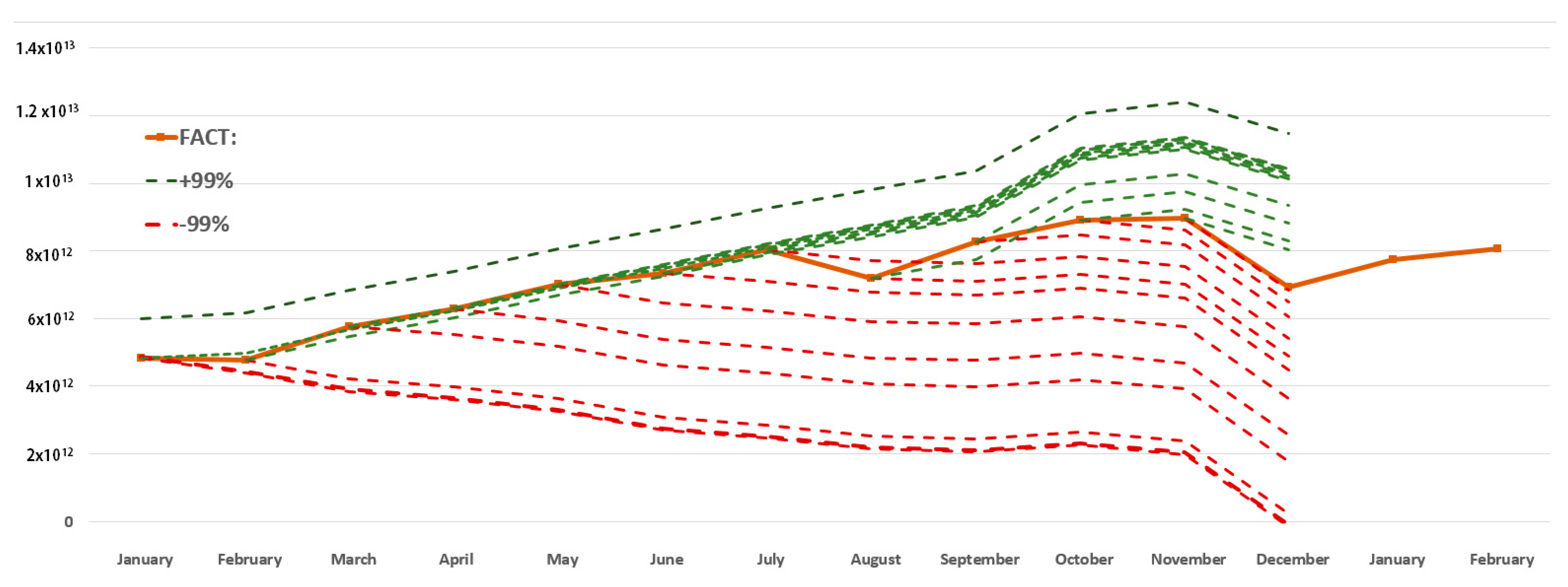
Using historical data for the period 2015–2020, we can emulate the behavior of the system in 2020. By sequentially adding data for the next month to the system, we can extrapolate increasing series using moving averages, aggregating them into the final forecast with an interval of 99%. At the output (Figure 2), we can obtain 11 pairs of upper and lower intervals, respectively, in the form of a set of separate rows with dimensions from 11 points to 1 point.
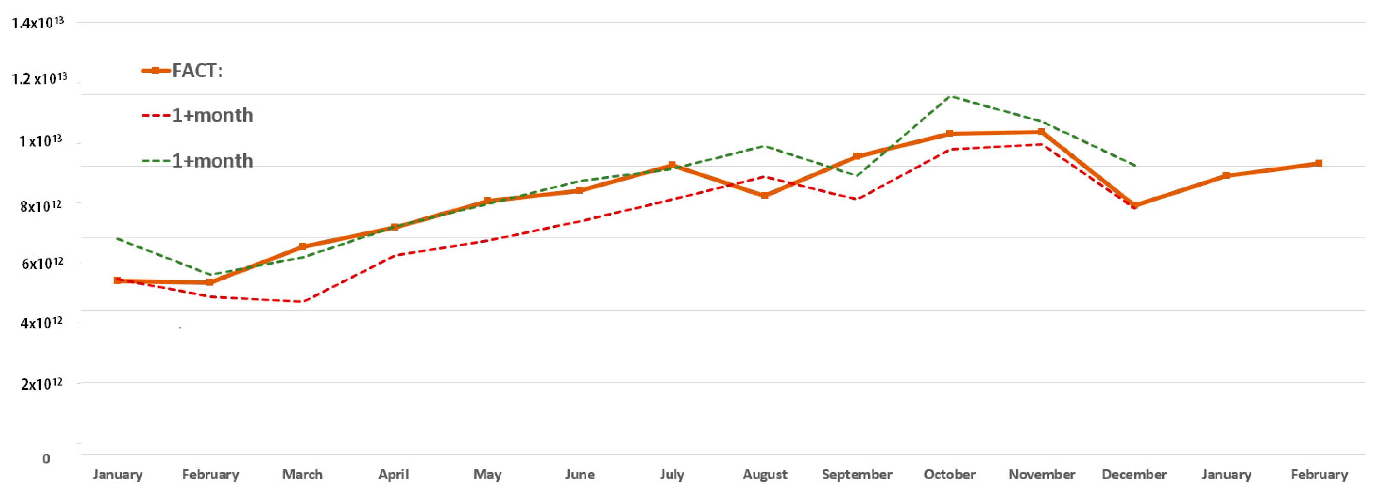
By combining the neighboring first points of the upper and lower rows of the confidence intervals, we can obtain a set of intervals (corridor) in which the actual values of the final prediction should be located (Figure 3).
As can be observed from Figure 3, despite the roughness of the model, the actual data of the residual on the EKC during the experiment extended beyond the lower limit of the interval once in August 2020.

5. Conclusions

It is possible to define a new class of systems dynamic models, in which the parameters are functions without uncertainties, and the solution is an interval. In addition, this is the first time that the prediction interval has been analyzed in this way, but this view is based on many modern studies, which we showed in this review.
In this review, we also presented a geometric view on the questions surrounding building an interval prediction. We can use graphs (solutions to evolutionary equations or solutions obtained in the course of machine learning of artificial neural networks) as objects that describe the same process in intervals with a given degree of deviation from the initial data, on the basis of which the model was trained.

Author Contributions

Conceptualization, E.N.; methodology, A.C.; software, A.C.; validation, E.N. and A.C.; formal analysis, E.N. and A.C.; data curation, A.C.; writing—original draft preparation, E.N. and A.C.; visualization, A.C. All authors have read and agreed to the published version of the manuscript.

Funding

This research received no external funding.

Data Availability Statement

Not applicable.

Conflicts of Interest

The authors declare no conflict of interest.

Abbreviations

AIArtificial intelligence
ARIMAAutoregressive integrated moving average model
ARMAAutoregressive moving average model
LSTMLong short-term memory
LUBELower upper bound estimation
MAPEMean absolute percentage error
PICPPrediction interval coverage probability
PINAWPrediction interval normalized average width
PIPrediction interval

References

  1. Zeng, Z.; Li, M. Bayesian median autoregression for robust time series forecasting. Int. J. Forecast. 2021, 37, 1000–1010. [Google Scholar] [CrossRef]
  2. Jeon, Y.; Seong, S. Robust recurrent network model for intermittent time-series forecasting. Int. J. Forecast. 2022, 38, 1415–1425. [Google Scholar] [CrossRef]
  3. Liu, Z.; Liu, J. A robust time series prediction method based on empirical mode decomposition and high-order fuzzy cognitive maps. Knowl. Based Syst. 2020, 203, 106105. [Google Scholar] [CrossRef]
  4. Hewamalage, H.; Bergmeir, C.; Bandara, K. Recurrent neural networks for time series forecasting: Current status and future directions. Int. J. Forecast. 2021, 37, 388–427. [Google Scholar] [CrossRef]
  5. Feizollahi, M.J.; Modarres, M. The robust deviation redundancy allocation problem with interval component reliabilities. IEEE Trans. Reliab. 2012, 61, 957–965. [Google Scholar] [CrossRef]
  6. Bochkov, A.V.; Lesnykh, V.V.; Zhigirev, N.N. Dynamic multi-criteria decision making method for sustainability risk analysis of structurally complex techno-economic systems. Reliab. Theory Appl. 2012, 7, 36–42. [Google Scholar]
  7. Zhou, M.; Wang, B.; Guo, S.; Watada, J. Multi-objective prediction intervals for wind power forecast based on deep neural networks. Inf. Sci. 2021, 550, 207–220. [Google Scholar] [CrossRef]
  8. Zhang, Z.; Ye, L.; Qin, H.; Liu, Y.; Li, J. Wind speed prediction method using shared weight long short-term memory network and Gaussian process regression. Appl. Energy 2019, 247, 270–284. [Google Scholar] [CrossRef]
  9. Ghimire, S.; Deo, R.C.; Wang, H.; Al-Musaylh, M.S.; Casillas-Pérez, D.; Salcedo-Sanz, S. Stacked LSTM sequence-to-sequence autoencoder with feature selection for daily solar radiation prediction: A review and new modeling results. Energies 2022, 15, 1061. [Google Scholar] [CrossRef]
  10. Jiang, F.; Zhu, Q.; Tian, T. An ensemble interval prediction model with change point detection and interval perturbation-based adjustment strategy: A case study of air quality. Expert Syst. Appl. 2023, 222, 119823. [Google Scholar] [CrossRef]
  11. Guan, Y.; Li, D.; Xue, S.; Xi, Y. Feature-fusion-kernel-based Gaussian process model for probabilistic long-term load forecasting. Neurocomputing 2021, 426, 174–184. [Google Scholar] [CrossRef]
  12. Zhang, W.; Quan, H.; Srinivasan, D. Parallel and reliable probabilistic load forecasting via quantile regression forest and quantile determination. Energy 2018, 160, 810–819. [Google Scholar] [CrossRef]
  13. Wan, C.; Xu, Z.; Pinson, P.; Dong, Z.Y.; Wong, K.P. Probabilistic forecasting of wind power generation using extreme learning machine. IEEE Trans. Power Syst. 2014, 29, 1033–1044. [Google Scholar] [CrossRef] [Green Version]
  14. Marín, L.G.; Cruz, N.; Sáez, D.; Sumner, M.; Núñez, A. Prediction interval methodology based on fuzzy numbers and its extension to fuzzy systems and neural networks. Expert Syst. Appl. 2019, 119, 128–141. [Google Scholar] [CrossRef] [Green Version]
  15. Yuan, X.; Chen, C.; Jiang, M.; Yuan, Y. Prediction interval of wind power using parameter optimized beta distribution based LSTM model. Appl. Soft. Comput. 2019, 82, 105550. [Google Scholar] [CrossRef]
  16. van der Meer, D.W.; Shepero, M.; Svensson, A.; Widén, J.; Munkhammar, J. Probabilistic forecasting of electricity consumption, photovoltaic power generation and net demand of an individual building using Gaussian Processes. Appl. Energy 2018, 213, 195–207. [Google Scholar] [CrossRef]
  17. Shepero, M.; van der Meer, D.W.; Munkhammar, J.; Widén, J. Residential probabilistic load forecasting: A method using Gaussian process designed for electric load data. Appl. Energy 2018, 218, 159–172. [Google Scholar] [CrossRef]
  18. van der Meer, D.W.; Munkhammar, J.; Widén, J. Probabilistic forecasting of solar power, electricity consumption and net load: Investigating the effect of seasons, aggregation and penetration on prediction intervals. Sol. Energy 2018, 171, 397–413. [Google Scholar] [CrossRef]
  19. Serrano-Guerrero, X.; Briceño-León, M.; Clairand, J.M.; Escrivá-Escrivá, G. A new interval prediction methodology for short-term electric load forecasting based on pattern recognition. Appl. Energy 2021, 297, 117173. [Google Scholar] [CrossRef]
  20. He, Y.; Liu, R.; Li, H.; Wang, S.; Lu, X. Short-term power load probability density forecasting method using kernel-based support vector quantile regression and Copula theory. Appl. Energy 2017, 185, 254–266. [Google Scholar] [CrossRef] [Green Version]
  21. He, Y.; Zheng, Y. Short-term power load probability density forecasting based on Yeo-Johnson transformation quantile regression and Gaussian kernel function. Energy 2018, 154, 143–156. [Google Scholar] [CrossRef]
  22. Zhang, H.; Zimmerman, J.; Nettleton, D.; Nordman, D.J. Random forest prediction intervals. Am. Stat. 2020, 74, 392–406. [Google Scholar] [CrossRef]
  23. He, F.; Zhou, J.; Mo, L.; Feng, K.; Liu, G.; He, Z. Day-ahead short-term load probability density forecasting method with a decomposition-based quantile regression forest. Appl. Energy 2019, 262, 114396. [Google Scholar] [CrossRef]
  24. Liu, F.; Li, C.; Xu, Y.; Tang, G.; Xie, Y. A new lower and upper bound estimation model using gradient descend training method for wind speed interval prediction. Wind. Energy 2021, 24, 290–304. [Google Scholar] [CrossRef]
  25. Taormina, R.; Chau, K.W. ANN-based interval forecasting of streamflow discharges using the LUBE method and MOFIPS. Eng. Appl. Artif. Intell. 2015, 45, 429–440. [Google Scholar] [CrossRef]
  26. Khosravi, A.; Nahavandi, S.; Creighton, D.; Atiya, A.F. Lower upper bound estimation method for construction of neural network-based prediction intervals. IEEE Trans. Neural Netw. Learn. Syst. 2011, 22, 337–346. [Google Scholar] [CrossRef]
  27. Quan, H.; Srinivasan, D.; Khosravi, A. Short-term load and wind power forecasting using neural network-based prediction intervals. IEEE Trans. Neural Netw. Learn. Syst. 2014, 25, 303–315. [Google Scholar] [CrossRef]
  28. Zhang, G.; Wu, Y.; Wong, K.P.; Xu, Z.; Dong, Z.Y.; Iu, H.H.C. An advanced approach for construction of optimal wind power prediction intervals. IEEE Trans. Power Syst. 2014, 30, 2706–2715. [Google Scholar] [CrossRef]
  29. Jiang, P.; Li, R.; Li, H. Multi-objective algorithm for the design of prediction intervals for wind power forecasting model. Appl. Math. Model. 2019, 67, 101–122. [Google Scholar] [CrossRef]
  30. Ak, R.; Vitelli, V.; Zio, E. An interval-valued neural network approach for uncertainty quantification in short-term wind speed prediction. IEEE Trans. Neural Netw. Learn. Syst. 2015, 26, 2787–2800. [Google Scholar] [CrossRef] [Green Version]
  31. Shrivastava, N.A.; Lohia, K.; Panigrahi, B.K. A multiobjective framework for wind speed prediction interval forecasts. Renew. Energy 2016, 87, 903–910. [Google Scholar] [CrossRef]
  32. Galván, I.M.; Valls, J.M.; Cervantes, A.; Aler, R. Multi-objective evolutionary optimization of prediction intervals for solar energy forecasting with neural networks. Inf. Sci. 2017, 418, 363–382. [Google Scholar] [CrossRef]
  33. Shi, Z.; Liang, H.; Dinavahi, V. Direct interval forecast of uncertain wind power based on recurrent neural networks. IEEE Trans. Sustain. Energy 2018, 9, 1177–1187. [Google Scholar] [CrossRef]
  34. Chen, X.; Lai, C.S.; Ng, W.W.; Pan, K.; Lai, L.L.; Zhong, C. A stochastic sensitivity-based multi-objective optimization method for short-term wind speed interval prediction. Int. J. Mach. Learn. Cybern. 2021, 12, 2579–2590. [Google Scholar] [CrossRef]
  35. Cao, Z.; Wan, C.; Zhang, Z.; Li, F.; Song, Y. Hybrid ensemble deep learning for deterministic and probabilistic low-voltage load forecasting. IEEE Trans. Power Syst. 2019, 35, 1881–1897. [Google Scholar] [CrossRef]
  36. Yao, Z.; Wann, J.; Chen, J. Generalized maximum entropy based identification of graphical ARMA models. Automatica 2022, 141, 110319. [Google Scholar]
  37. Entezami, A.; Sarmadi, H.; Behkamal, B.; Mariani, S. Big data analytics and structural health monitoring: A statistical pattern recognition-based approach. Sensors 2020, 20, 2328. [Google Scholar] [CrossRef] [Green Version]
  38. Shi, Q.; Yin, J.; Cai, J.; Cichocki, A.; Yokota, T.; Chen, L.; Zeng, J. Block Hankel tensor ARIMA for multiple short time series forecasting. Proc. AAAI Conf. Artif. Intell. 2020, 34, 5758–5766. [Google Scholar] [CrossRef]
  39. Li, S.; Wang, P.; Goel, L. Wind power forecasting using neural network ensembles with feature selection. IEEE Trans Sustain. Energy 2015, 6, 1447–1456. [Google Scholar] [CrossRef]
  40. Luo, X.; Sun, J.; Wang, L.; Wang, W.; Zhao, W.; Wu, J.; Zhang, Z. Short-term wind speed forecasting via stacked extreme learning machine with generalized correntropy. IEEE Trans. Ind. Inform. 2018, 14, 4963–4971. [Google Scholar] [CrossRef] [Green Version]
  41. Jahangir, H.; Golkar, M.A.; Alhameli, F.; Mazouz, A.; Ahmadian, A.; Elkamel, A. Short-term wind speed forecasting framework based on stacked denoising auto-encoders with rough ANN. Sustain. Energy Technol. Assess. 2020, 38, 100601. [Google Scholar] [CrossRef]
  42. Messina, A.R.; Vittal, V. Nonlinear, non-stationary analysis of interarea oscillations via Hilbert spectral analysis. IEEE Trans. Power Syst. 2006, 21, 1234–1241. [Google Scholar] [CrossRef]
  43. Leung, T.; Zhao, T. Financial time series analysis and forecasting with Hilbert–Huang transform feature generation and machine learning. Appl. Stoch. Model. Bus. Ind. 2021, 37, 993–1016. [Google Scholar] [CrossRef]
  44. Liu, Z.; Jiang, P.; Zhang, L.; Niu, X. A combined forecasting model for time series: Application to short-term wind speed forecasting. Appl. Energy 2020, 259, 114137. [Google Scholar] [CrossRef]
  45. Ahmadi, G.; Teshnehlab, M. Designing and implementation of stable sinusoidal rough-neural identifier. IEEE Trans. Neural. Netw. Learn. Syst. 2017, 28, 1774–1786. [Google Scholar] [CrossRef]
  46. Jiang, P.; Li, R.; Li, H.J. A combined model based on data preprocessing strategy and multi-objective optimization algorithm for short-term wind speed forecasting. Appl. Energy 2019, 241, 519–539. [Google Scholar]
  47. Alsharekh, M.F.; Habib, S.; Dewi, D.A.; Albattah, W.; Islam, M.; Albahli, S. Improving the Efficiency of Multistep Short-Term Electricity Load Forecasting via R-CNN with ML-LSTM. Sensors 2022, 22, 6913. [Google Scholar] [CrossRef]
  48. Kabir, H.D.; Khosravi, A.; Hosen, M.A.; Nahavandi, S. Neural network-based uncertainty quantification: A survey of methodologies and applications. IEEE Access 2018, 6, 36218–36234. [Google Scholar] [CrossRef]
  49. Hong, T.; Fan, S. Probabilistic electric load forecasting: A tutorial review. Int. J. Forecast. 2016, 32, 914–938. [Google Scholar] [CrossRef]
  50. Pluzhnik, E.; Nikulchev, E. Virtual laboratories in cloud infrastructure of educational institutions. In Proceedings of the 2014 2nd 2014 2nd International Conference on Emission Electronics (ICEE), Saint-Petersburg, Russia, 30 June–4 July 2014; pp. 1–3. [Google Scholar]
  51. Nikulchev, E.V. Simulation of robust chaotic signal with given properties. Adv. Stud. Theor. Phys. 2014, 8, 939–944. [Google Scholar] [CrossRef]
  52. Nikulchev, E. Robust chaos generation on the basis of symmetry violations in attractors. In Proceedings of the 2014 2nd International Conference on Emission Electronics (ICEE), Saint-Petersburg, Russia, 30 June–4 July 2014; pp. 1–3. [Google Scholar]
  53. Koppe, G.; Toutounji, H.; Kirsch, P.; Lis, S.; Durstewitz, D. Identifying nonlinear dynamical systems via generative recurrent neural networks with applications to fMRI. PLoS Comput. Biol. 2019, 15, e1007263. [Google Scholar] [CrossRef] [PubMed]
  54. Gao, J.; Song, X.; Wen, Q.; Wang, P.; Sun, L.; Xu, H. Robusttad: Robust time series anomaly detection via decomposition and convolutional neural networks. arXiv 2020, arXiv:2002.09545. [Google Scholar]
  55. Rathnayaka, R.K.T.; Seneviratna, D.M.K.N. Taylor series approximation and unbiased GM (1, 1) based hybrid statistical approach for forecasting daily gold price demands. Grey Syst. Theory Appl. 2019, 9, 5–18. [Google Scholar] [CrossRef]
  56. Chaudhary, P.K.; Pachori, R.B. Automatic diagnosis of glaucoma using two-dimensional Fourier-Bessel series expansion based empirical wavelet transform. Biomed. Signal Process. Control. 2021, 64, 102237. [Google Scholar] [CrossRef]
  57. Son, J.H.; Kim, Y. Probabilistic time series prediction of ship structural response using Volterra series. Mar. Struct. 2021, 76, 102928. [Google Scholar] [CrossRef]
  58. Wu, S.; Xiao, X.; Ding, Q.; Zhao, P.; Wei, Y.; Huang, J. Adversarial sparse transformer for time series forecasting. Adv. Neural Inf. Process. Syst. 2020, 33, 17105–17115. [Google Scholar]
  59. Montagnon, C.E. Forecasting by splitting a time series using Singular Value Decomposition then using both ARMA and a Fokker Planck equation. Phys. A Stat. Mech. Its Appl. 2021, 567, 125708. [Google Scholar] [CrossRef]
  60. Khan, S.; Alghulaiakh, H. ARIMA model for accurate time series stocks forecasting. Int. J. Adv. Comput. Sci. Appl. 2020, 11, 524–528. [Google Scholar] [CrossRef]
  61. Lara-Benítez, P.; Carranza-García, M.; Riquelme, J.C. An experimental review on deep learning architectures for time series forecasting. Int. J. Neural Syst. 2021, 31, 2130001. [Google Scholar] [CrossRef]
  62. Sezer, O.B.; Gudelek, M.U.; Ozbayoglu, A.M. Financial time series forecasting with deep learning: A systematic literature review: 2005–2019. Appl. Soft Comput. 2020, 90, 106181. [Google Scholar] [CrossRef] [Green Version]
  63. Lim, B.; Zohren, S. Time-series forecasting with deep learning: A survey. Philos. Trans. R. Soc. A Math. Phys. Eng. Sci. 2021, 379, 20200209. [Google Scholar] [CrossRef] [PubMed]
  64. Meisenbacher, S.; Turowski, M.; Phipps, K.; Rätz, M.; Müller, D.; Hagenmeyer, V.; Mikut, R. Review of automated time series forecasting pipelines. Wiley Interdiscip. Rev. Data Min. Knowl. Discov. 2022, 12, e1475. [Google Scholar] [CrossRef]
  65. Astakhova, N.N.; Demidova, L.A.; Nikulchev, E.V. Forecasting of time series’ groups with application of fuzzy c-mean algorithm. Contemp. Eng. Sci. 2015, 8, 1659–1677. [Google Scholar] [CrossRef]
  66. Samokhin, A.B. Methods and effective algorithms for solving multidimensional integral equations. Russ. Technol. J. 2022, 10, 70–77. [Google Scholar] [CrossRef]
  67. Petrushin, V.N.; Nikulchev, E.V.; Korolev, D.A. Histogram Arithmetic under Uncertainty of Probability Density Function. Appl. Math. Sci. 2015, 9, 7043–7052. [Google Scholar] [CrossRef] [Green Version]
  68. Shi, Z.; Liang, H.; Dinavahi, V. Wavelet neural network based multiobjective interval prediction for short-term wind speed. IEEE Access 2018, 6, 63352–63365. [Google Scholar] [CrossRef]
  69. Khosravi, A.; Nahavandi, S.; Creighton, D. Construction of optimal prediction intervals for load forecasting problems. IEEE Trans. Power Syst. 2010, 25, 1496–1503. [Google Scholar] [CrossRef] [Green Version]
  70. Zhang, C.; Wei, H.; Xie, L.; Shen, Y.; Zhang, K. Direct interval forecasting of wind speed using radial basis function neural networks in a multi-objective optimization framework. Neurocomputing 2016, 205, 53–63. [Google Scholar] [CrossRef]
  71. Arora, P.; Jalali, S.M.J.; Ahmadian, S.; Panigrahi, B.K.; Suganthan, P.; Khosravi, A. Probabilistic wind power forecasting using optimised deep auto-regressive recurrent neural networks. IEEE Trans. Autom. Sci. Eng. 2023, 20, 271–284. [Google Scholar] [CrossRef]
  72. Wang, J.; Li, Q.; Zhang, H.; Wang, Y. A deep-learning wind speed interval forecasting architecture based on modified scaling approach with feature ranking and two-output gated recurrent unit. Expert Syst. Appl. 2023, 211, 118419. [Google Scholar] [CrossRef]
  73. Yeung, D.S.; Li, J.; Ng, W.W.Y.; Chan, P.P.K. MLPNN training via a multiobjective optimization of training error and stochastic sensitivity. IEEE Trans. Neural Netw. Learn. Syst. 2016, 27, 978–992. [Google Scholar] [CrossRef] [PubMed]
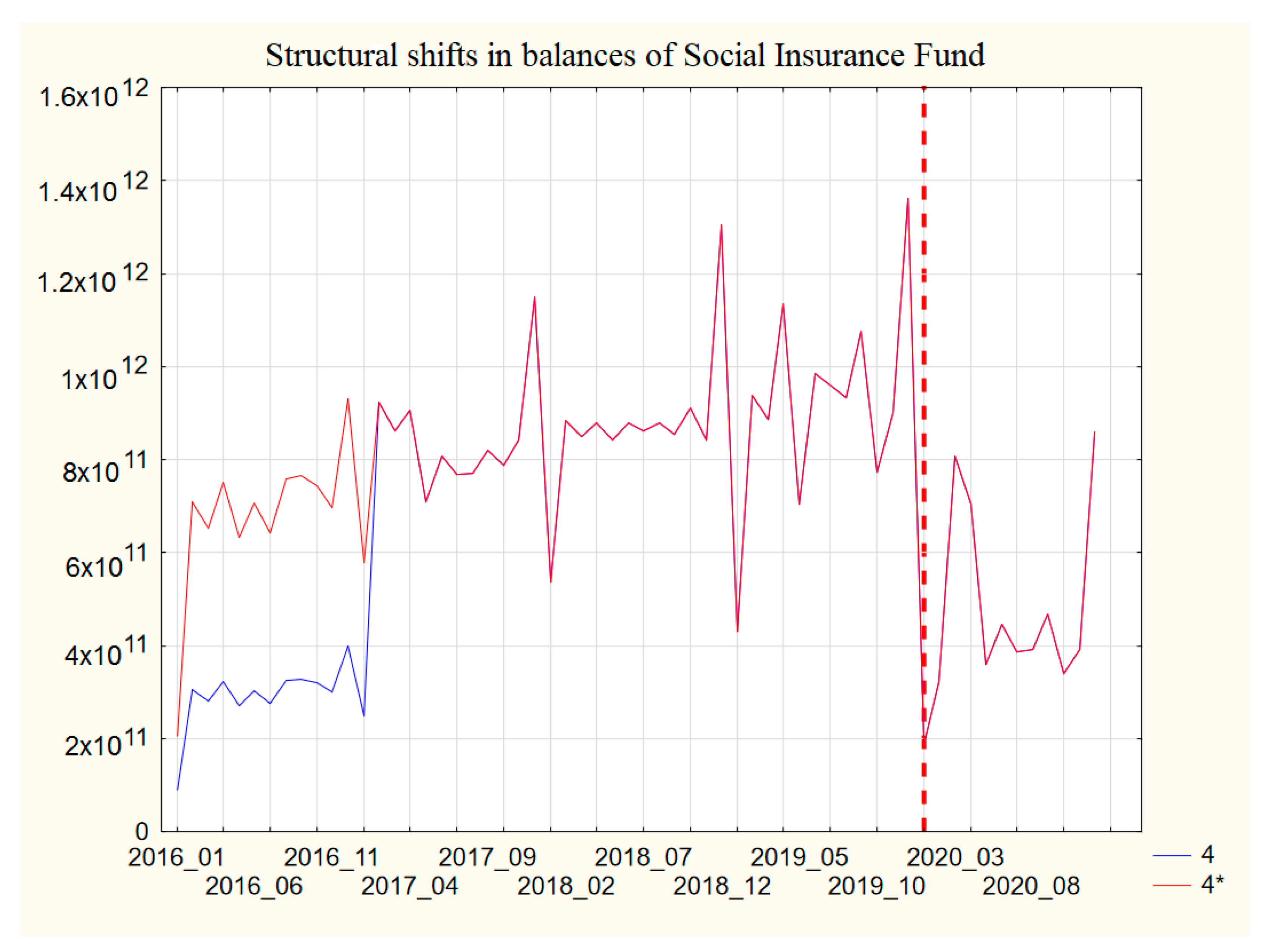
Figure 1. Structural shifts in the balances of the Social Insurance Fund.
Symmetry 15 00781 g001
Figure 2. Construction of a robust interval model in 2020.
Symmetry 15 00781 g002
Figure 3. Comparison of the robust interval model with actual data.
Symmetry 15 00781 g003
Table 1. Classification of series prediction methods.
ClassModel TypeAdvantagesDisadvantages
Direct modeling methods1.1. Engineering physical models- Can model any physical systemThey are complex and require detailed knowledge of the physical properties of the simulated process or device. Often unjustified high complexity
2.2. Parametric identification of dynamical systems [53]- Model parameters can be calculated from the initial data- For non-linear systems, knowledge of non-linearities is required. High sensitivity to variations in variables
Robust models- Insensitivity to small changesAmbiguity of decisions
Inverse methods (time series modeling)Series or expansions
(Fourier series [54], Taylor series [55], Bessel series [56], Volterra functional expansion [57], etc.)
Fast calculations and ease of useThere are no criteria for how many members of the series must be used. Demonstrates sensitivity to the types of non-linearities in dynamics
Regression methods
Linear regression, exponential regression [58], Box Jenkins (autoregressive moving average (ARMA) [59], autoregressive integrated moving average (ARIMA) [60]; Holt and Winters
Fast calculationsPoor prediction due to multiple seasonality of data. The art of choosing the right type of model is required
Stochastic models (Bayesian models, Gaussian models; beta distribution)Ease of use Tied to a distribution type
Machine learning [61,62,63,64]
Neural networks, deep learning, evolutionary algorithms [65], etc.
High precision and adaptabilityHigh dependence on the amount of training data
Combined deterministic and non-deterministic modelsA good criterion in choosing models improves predictions.
They support physical interpretations without the need for a very detailed or complex mathematical model
An expert is required to select the parameters of non-deterministic models.
Implementation can be difficult
Prediction intervalCombined methods, integral equations [66], histogram arithmetic [67]; methods for constructing intervals [68]Can use any of the above modelsOne is required to solve the problem of choosing the width of the interval
Disclaimer/Publisher’s Note: The statements, opinions and data contained in all publications are solely those of the individual author(s) and contributor(s) and not of MDPI and/or the editor(s). MDPI and/or the editor(s) disclaim responsibility for any injury to people or property resulting from any ideas, methods, instructions or products referred to in the content.