Parameter Estimation in the Mathematical Model of Bacterial Colony Patterns in Symmetry Domain

Abstract

The paper presents a solution to the problem related to the reconstruction of parameters in the mathematical model of bacterial colony patterns in a domain with symmetry. The inverse problem consists of determining the value of the diffusion coefficient of active bacteria. The model describing the distribution of active bacteria in a given region, as well as the concentration of the substrate over time is considered. Such a model consists of a system of partial differential equations with appropriate initial-boundary conditions. The finite element method was used to solve the direct problem. However, the Fibonacci search method was used to minimize the functional description of the error of the approximate solution.

1. Introduction

Each ecosystem on the Earth is inhabited by communities of bacteria and other microorganisms. They occur on the surfaces of objects, in soil, and in water, and they live in the body of humans and animals. They often form on surfaces dense colonies called biofilms. Its structure of it depends on physical, chemical and biological factors. Among the many specific factors of growth and functioning of the colony, the most important should be access to water and nutrients, and the characteristics of the substrate [1,2,3].

Most biofilms found in nature are mixtures of different species of bacteria. In such cases, competition for a specific ecological niche is most often observed. When studying single-species biofilm, the development of a given colony can be observed depending on the variety of environmental conditions. A common microorganism used in bacterial colony studies is the Gram-positive bacterium Bacillus subtilis. It is a model organism, in particular, used to observe the formation of biofilm by bacteria and the way bacteria move in various environments and on various substrates [1,2,4]. This type of bacteria is quite widespread and also does not show pathogenic properties in the basic form. B. subtilis is an important component of the human microflora, it is present, inter alia, on the skin surface and in the gastrointestinal tract. It is a symbiote that produces a compound called bacitracin, which inhibits the growth of other Gram-positive bacteria. As a result, these bacteria are used in the pharmaceutical industry [2,5,6].

Experimental and mathematical modeling is an important study of bacterial colonies with regard to their application in various branches of the economy. Due to the fact that B. subtilis is a bacterium that differentiates quickly and shows the possibility of various types of motility, the microorganism can be used to model the behavior of Gram-positive bacteria, in general, [5,7]. Modeling the behavior of B. subtilis, as for example, in the papers [8,9,10,11], change the behavior of the colony depending on the parameters of the environment. The adaptive abilities of bacteria allow the observation of various types of motility, communication and reproduction methods. As a result, it is possible to determine the mechanisms shaping the desired development of bacterial colonies and the patterns adopted by them, which is conducive to the optimization of biological research and production of substances using Gram-positive bacteria [8,9,10,11].

Inverse problems have an important role in science. Solving inverse problems of various kinds allows for more accurate modeling of various processes [12,13,14,15,16,17,18]. For example, in [12], authors compared various mathematical models of heat conduction based on temperature measurements of porous aluminum. In order to perform the comparison, an inverse problem had to be solved, consisting in identifying several model coefficients. The Ant Colony Optimization algorithm was used to solve this problem. In paper [14] a novel spatially and temporally controlled heating method was proposed. The laser configuration was achieved by solving the inverse heat conduction problem. In papers [17,18] from the knowledge of temperature measurements the aerothermal heating of a reusable launch vehicle is reconstructed. For solving the direct problem the implicit scheme of the finite difference method is used, whereas the solution to the inverse problem is determined with the aid of the Levenberg–Marquardt method. More about inverse problems can be found in [19,20,21].

Examples of the application of inverse problems in biological sciences can be found in the papers [22,23,24,25,26]. Abdulla and Poteau in paper [23] describe the identification of parameters for a model of a biological system described by a system of nonlinear ordinary differential equations. The presented method is a combination of Bellman’s quasilinearization, Tikhonov’s regularization and sensitivity coefficients. The examples in the article concern the Lotka–Volterra model, the bistable switch model in genetic regulatory networks, gene regulation and repressilator models from synthetic biology. However, Capasso et al. [24] describes the application of Barnsley’s Collage Theorem [27] to solve the inverse problem for the model described by first-order ordinary differential equations. In the examples, the following models are considered: population dynamics, mRNA and protein concentration, bacteria and amoeba cells interaction, and tumor growth. Models described by the system of ordinary differential equations are also considered by Kabanikhin and Krivorotko [25]. This time the solution was based on the gradient method. Numerical examples concerned models of infectious disease, HIV dynamics, and the spread of tuberculosis. In the inverse problem considered by Doumic et al. [26], the division rate from the cell volume distribution data in certain structured population models is reconstructed. The quasi-reversibility method and filtering method were used in the calculations. In paper [28] a novel 2-hydr_Ensemble residues’ identification algorithm was proposed. Several typical classification models can be employed to compare. Presented algorithm has the ability to find out the potential information among several feature vectors. Paper [29] focuses on the application of a capsule network (CapsNet) to identify the pneumonia-related compounds in Qingre Jiedu injection. Obtained results show that CapsNet can identify disease-related compounds more accurately than other methods like SVM or RF. In the work [30], the authors propose and develop a tool called Phage_UniR_LGBM to classify the virion proteins.

In mathematical modeling, it is very important to properly determine the values of parameters in the model. Some of these parameters cannot be accurately determined on the basis of theory or direct measurements. In that case, we can try to measure a different quantity and then solve the inverse problem of identifying the value of the parameter we are interested in. Such an inverse problem is considered in this paper. Namely on the basis of the knowledge density of active bacteria at a given point the diffusion coefficient of active bacteria is determined. This paper considers a model describing the density distribution of B. subtilis as well as the concentration of the substrate. A model consisting of two non-linear partial differential equations is considered. The assumed symmetry consists of the fact that homogeneous boundary conditions of the second kind are given for both functions on the boundary of the area. Thus, there is no flow of bacteria or substrate through the boundary of the area. As a consequence, the obtained solution to the direct problem can be symmetrically reflected with respect to the boundary of the region (analog to thermal symmetry). The finite element method was used to solve the direct problem. However, to determine the minimum of the functional, describing the error of the approximate solution, the Fibonacci search method was used. The inverse problem was solved for different noises of the input data.

2. Bacterial Colonies Model

In this section, a model of a bacterial colony is presented, which is describing the distribution of active bacteria in space and time and the concentration of the substrate (nutrient field). Both, bacteria cells and the nutrient, diffuse when bacteria cells multiply by consuming nutrients. We assume that the distribution of active bacteria and concentration of the substrate meets the conditions of symmetry. Therefore, it is possible to consider a fragment of the entire area with symmetry conditions set on the boundary. We consider region $\mathrm{\Omega }=\{(x,y):x\in (x_l,x_r),y\in (y_l,y_r)\}$ where $-\infty <x_l<x_r<\infty$ and $-\infty <y_l<y_r<\infty$ for time $t\in [0,t^{*}]$. By b we denote the density of active bacteria and by s concentration of substrate. Their distribution is described by the system of partial differential Equations [31]:

$$\begin{array}{cc}\hfill \frac{\partial b}{\partial t}& =\nabla \left(D_b(b,s)\nabla b\right)-\nabla \left(\chi \left(s\right)b\nabla s\right)+g\left(s\right)b,\hfill \end{array}$$

(1)

$$\begin{array}{cc}\hfill \frac{\partial s}{\partial t}& =D_s{\nabla }^{2}s-g\left(s\right)b,\hfill \end{array}$$

(2)

where $D_b(b,s)$ is nonlinear diffusion for bacterial cells, $\chi \left(s\right)$ is chemotactic response, $g\left(s\right)$ is function describing specific bacterial growth rate and $D_s$ is constant diffusion coefficient for substrate. The first term of Equation (1) describes the motility, the second mortality and the third reproduction. Using the equations, it is possible to model different types of bacterial motility, such as swimming, sliding and swarming, as well as the motility of a single bacterium, in smaller clusters or larger agglomerates [5,8]. It is also possible to determine the conditions of secretion of substances by bacteria and the formation of various patterns, such as a ring pattern, resulting from cyclical changes in the differentiation of bacteria from swimming to swarming forms [8,9,10].

To the system of differential Equation (1) and (2) the initial conditions are posed:

$$\begin{array}{cccc}\hfill b(x,y,0)& =b_0(x,y),\hfill & \hfill & \mathrm{for}(x,y)\in \mathrm{\Omega },\hfill \end{array}$$

(3)

$$\begin{array}{ccc}\hfill s(x,y,0)& =v_0,\hfill & \mathrm{for}(x,y)\in \mathrm{\Omega }.\hfill \end{array}$$

(4)

Due to the assumed symmetry, on the boundary $\partial \mathrm{\Omega }$ of the $\mathrm{\Omega }$, homogeneous boundary conditions of the second kind are set:

$$\begin{array}{cccc}\hfill \frac{\partial b}{\partial n}(x,y,t)& =0,\hfill & \hfill & \mathrm{for}(x,y)\in \partial \mathrm{\Omega },t\in [0,t^{*}],\hfill \end{array}$$

(5)

$$\begin{array}{cccc}\hfill \frac{\partial s}{\partial n}(x,y,t)& =0,\hfill & \hfill & \mathrm{for}(x,y)\in \partial \mathrm{\Omega },t\in [0,t^{*}].\hfill \end{array}$$

(6)

In the presented model, we assume [31,32]:

$$\begin{array}{cc}\hfill D_b(b,s)& =Dbs,\hfill \end{array}$$

(7)

$$\begin{array}{cc}\hfill g\left(s\right)& =k\frac{s}{1+s},\hfill \end{array}$$

(8)

$$\begin{array}{cc}\hfill \chi \left(s\right)& =vs.\hfill \end{array}$$

(9)

where D is linear diffusion coefficient for bacterial cells, v is chemotaxis coefficient and k is arbitrary constant. Taking into account (7)–(9), system of differential Equations (1) and (2) has following form:

$$\begin{array}{cc}\hfill \frac{\partial b}{\partial t}& =D\left(\frac{\partial }{\partial x}\left(bs\frac{\partial b}{\partial x}\right)+\frac{\partial }{\partial y}\left(bs\frac{\partial b}{\partial y}\right)\right)-v\left(\frac{\partial }{\partial x}\left(bs\frac{\partial s}{\partial x}\right)+\frac{\partial }{\partial y}\left(bs\frac{\partial s}{\partial y}\right)\right)+k\frac{bs}{1+s},\hfill \end{array}$$

(10)

$$\begin{array}{cc}\hfill \frac{\partial s}{\partial t}& =D_s\left(\frac{{\partial }^{2}s}{\partial x^2}+\frac{{\partial }^{2}s}{\partial y^2}\right)-k\frac{bs}{1+s}.\hfill \end{array}$$

(11)

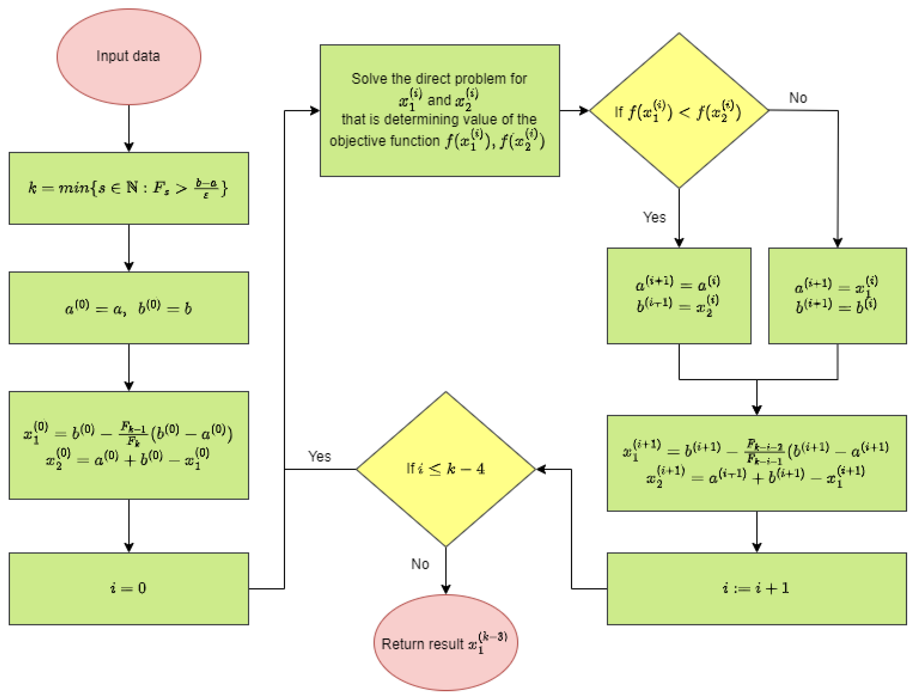
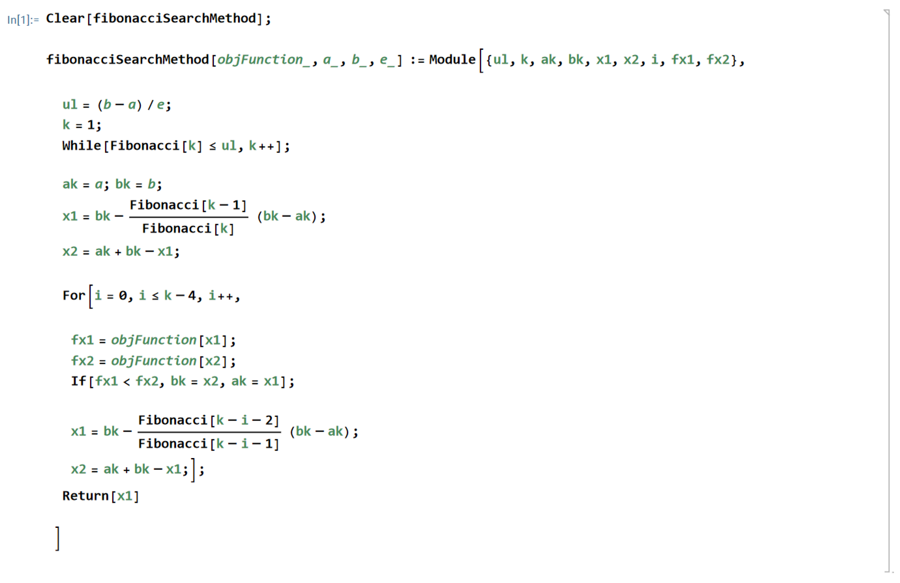
3. Inverse Problem and Its Solution

In this section, we consider the inverse problem which consists of reconstructing the value of diffusion coefficient D. Additional information which we used for the identification of the D coefficient is the values of the b function (density of active bacteria) in a given point in the $\mathrm{\Omega }$ region. We denote this data by $\overline{b}(x_p,y_p,t_i)$, where $(x_p,y_p)\in \mathrm{\Omega }$ are the coordinates of the measuring point, and $t_i$, $i=1,2,\dots ,N$, are measurement times. By solving the direct problem for a fixed value of the coefficient D (solving the system of Equations (1) and (2)), we obtain the values of the b function in the measuring point—$b_D(x_p,y_p,t_i)$. Next, by comparing the data obtained from the model for the given D coefficient $b_D(x_p,y_p,t_i)$ with the measurement data $\overline{b}(x_p,y_p,t_i)$, we create a function describing the error of approximate solution:

$$J\left(D\right)=\sum _{i=1}^N{\left(b_D(x_p,y_p,t_i)-\overline{b}(x_p,y_p,t_i)\right)}^2.$$

(12)

By minimizing the above objective function, we can identify the approximate value of the D coefficient.

In order to solve the direct problem, the finite element method supplemented with the method of lines was used. In the case of determining the minimum of the objective function, the Fibonacci search method [33,34] was used. Now, we present the algorithm of the Fibonacci search method.

1.

Input: objective function f (unimodal function),

•        interval $[a,b]$,
•        required absolute precision $\epsilon$.

2.

Determine the smallest number $k\in \mathbb{N}$ for which $F_k>\frac{b-a}{\epsilon }$, where $F_k$ is the Fibonacci number.

3.

Set $a^{\left(0\right)}=a$ and $b^{\left(0\right)}=b$.

4.

Determine $x_1^{\left(0\right)}=b^{\left(0\right)}-\frac{F_{k-1}}{F_k}\left(b^{\left(0\right)}-a^{\left(0\right)}\right)$ and $x_2^{\left(0\right)}=a^{\left(0\right)}+b^{\left(0\right)}-x_1^{\left(0\right)}$.

5.

For $i=0,1,\dots ,k-4$:

5a.

If $f(x_1^{\left(i\right)})<f(x_2^{\left(i\right)})$, then $a^{(i+1)}=a^{\left(i\right)}$ and $b^{(i+1)}=x_2^{\left(i\right)}$,

otherwise $a^{(i+1)}=x_1^{\left(i\right)}$ and $b^{(i+1)}=b^{\left(i\right)}$.

5b.

Determine

$$\begin{array}{cc}\hfill x_1^{(i+1)}& =b^{(i+1)}-\frac{F_{k-i-2}}{F_{k-i-1}}\left(b^{(i+1)}-a^{(i+1)}\right),\hfill \\ \hfill x_2^{(i+1)}& =a^{(i+1)}+b^{(i+1)}-x_1^{(i+1)}.\hfill \end{array}$$

6.

Result $x_1^{(k-3)}$.

The designed algorithm was implemented in Wolfram language on Mathematica 12.3 platform [35] and the calculations were performed by using the computer with processor Intel Core i7-8565U, 1.80 Ghz, 2.00 GHz, equipped with 16 GB RAM memory.

The block diagram of the calculation procedure is shown in Figure 1. However, the implementation of the Fibonacci search method in Wolfram language [35] is shown in Figure 2. In each step of the procedure for solving the inverse problem the values of the objective function should be determined in consecutive points $x_1^i$ and $x_2^i$. This is related to the solution of the direct problem composed of Equations (10) and (11) with boundary conditions (3)–(6). Solving single direct problem took about $2.7$ s, while solving inverse problem took about $130$ s.

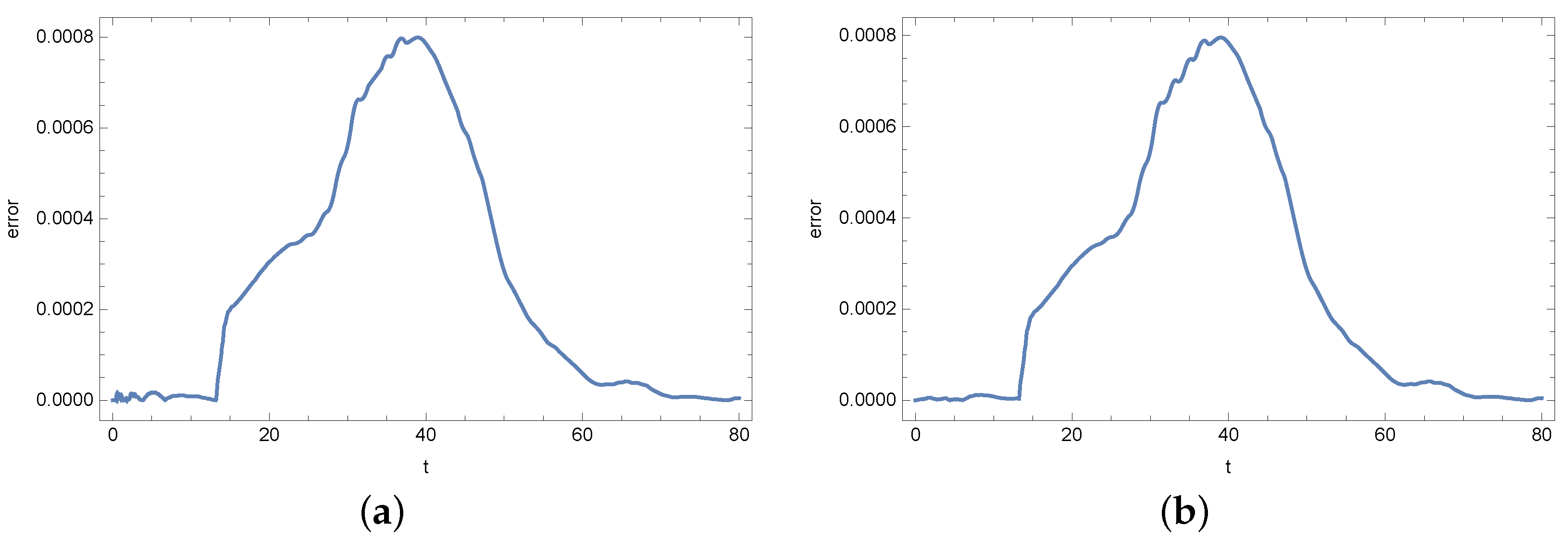
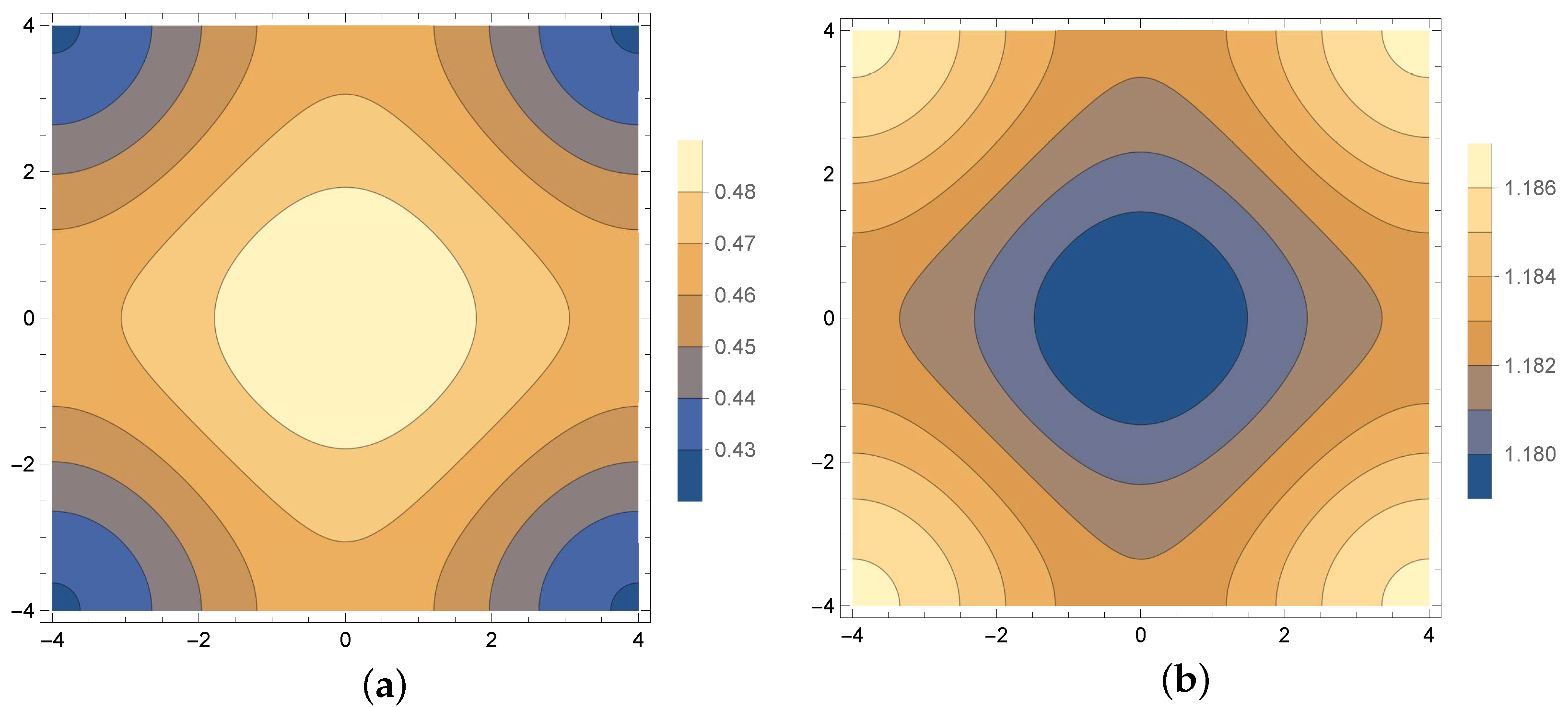
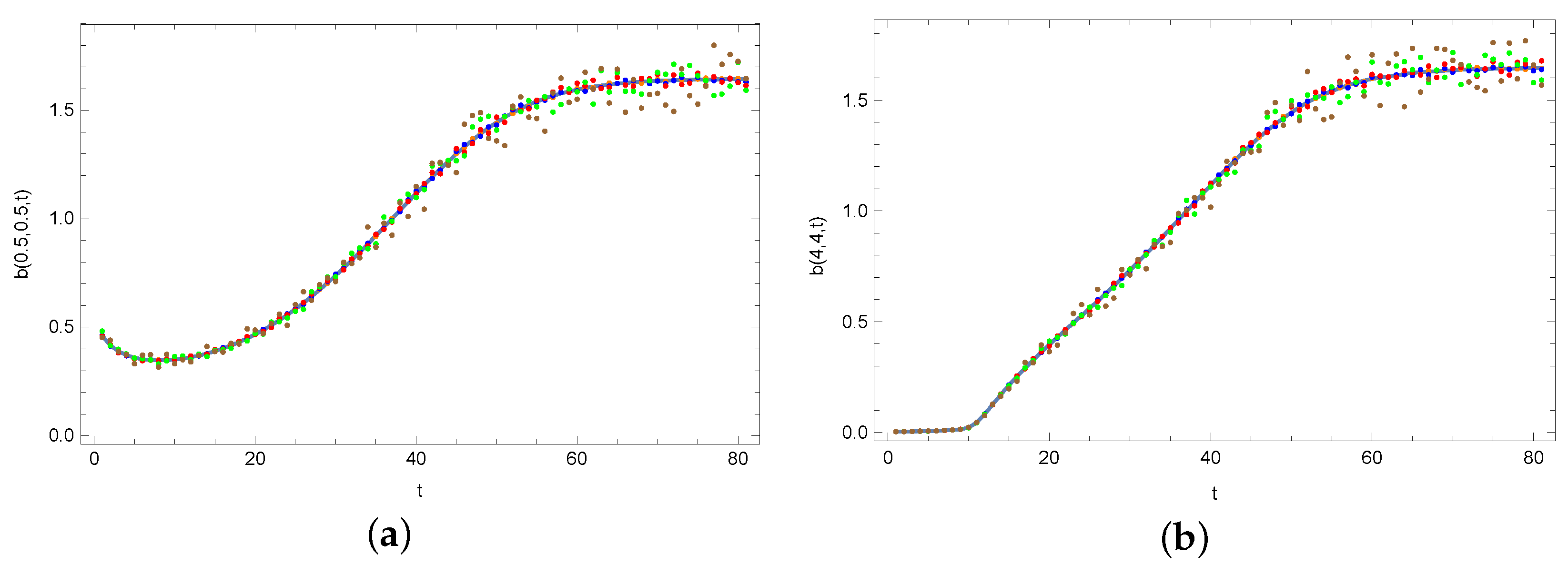
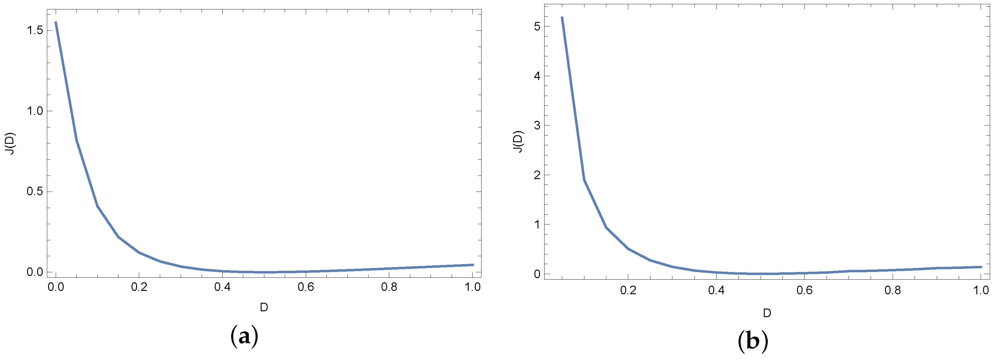
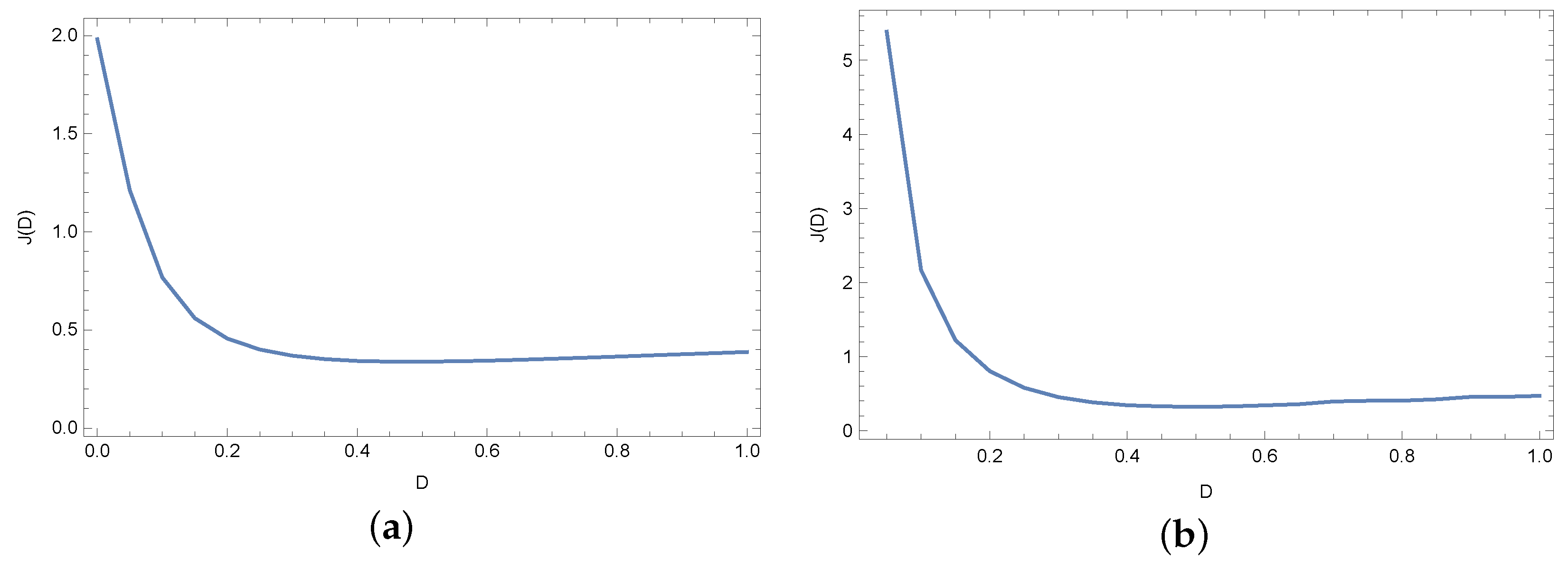
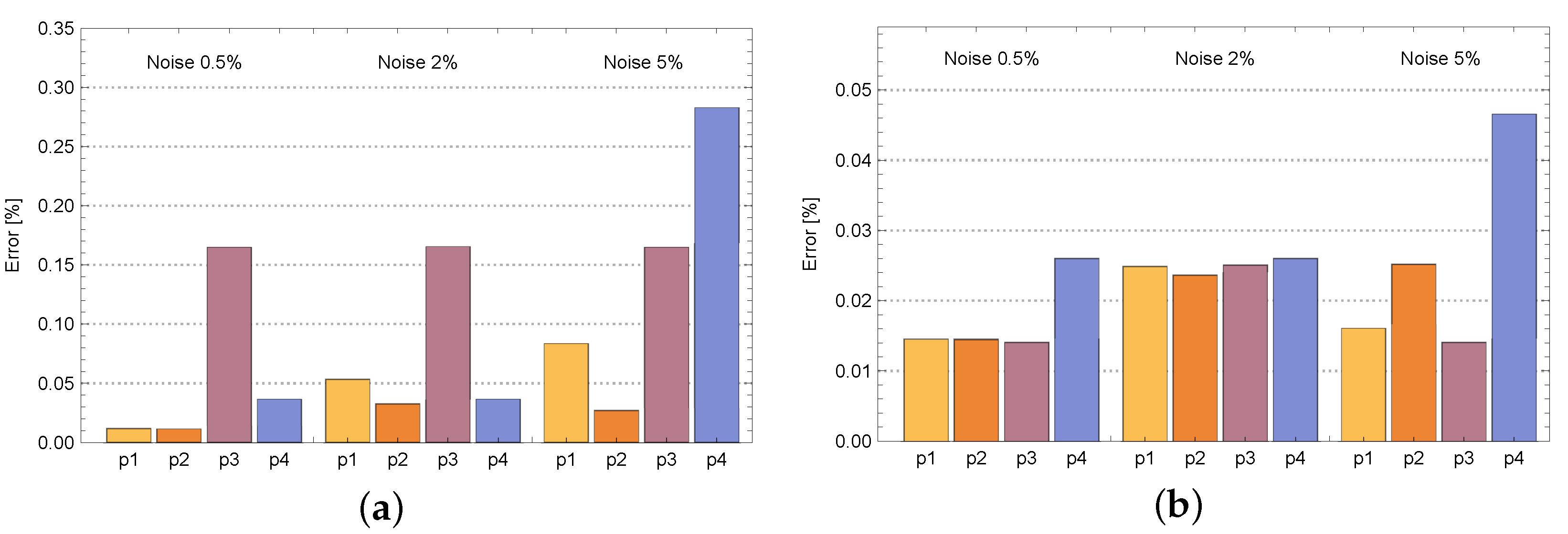
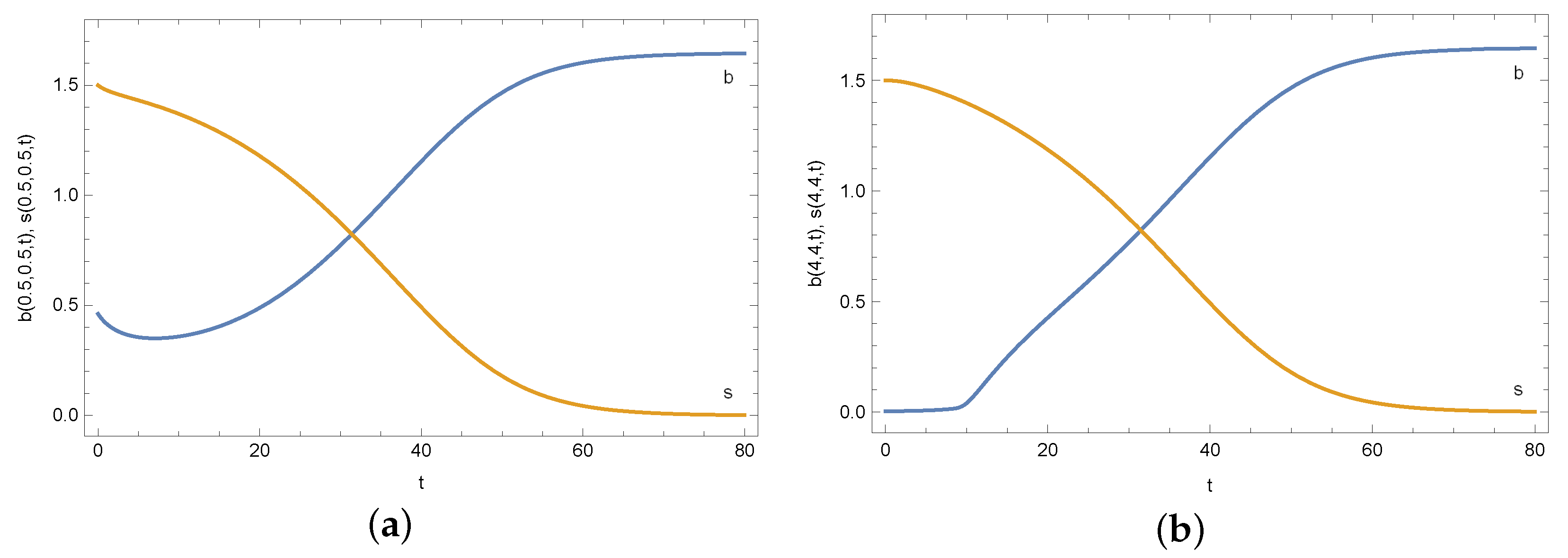
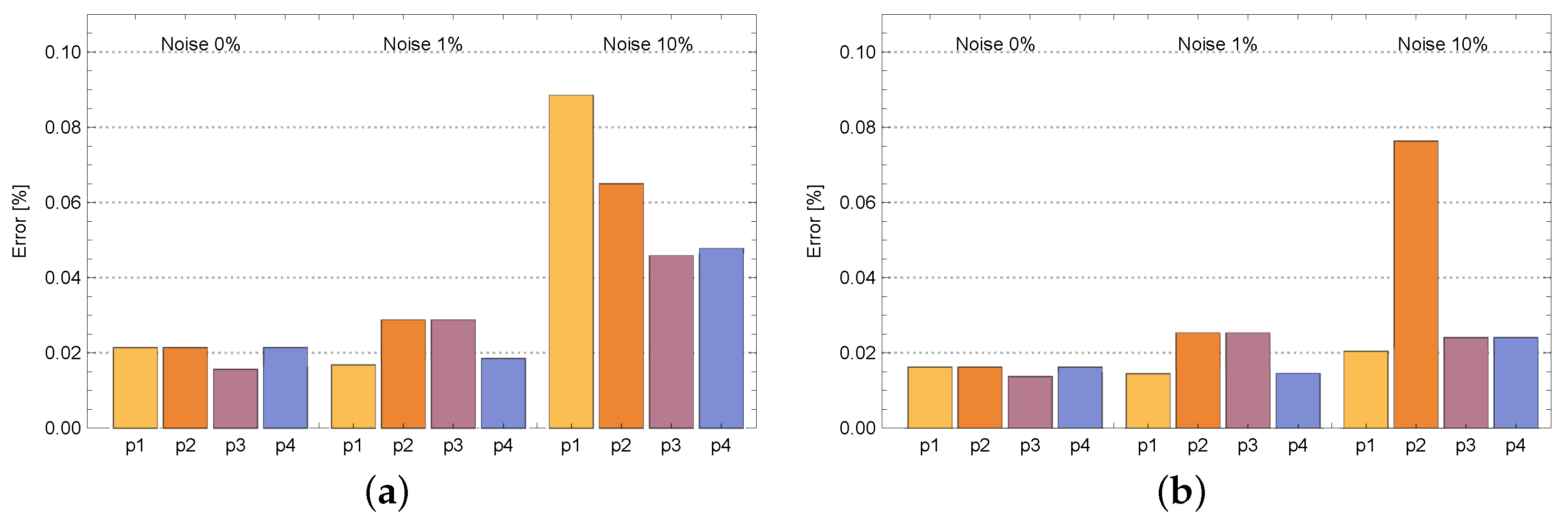
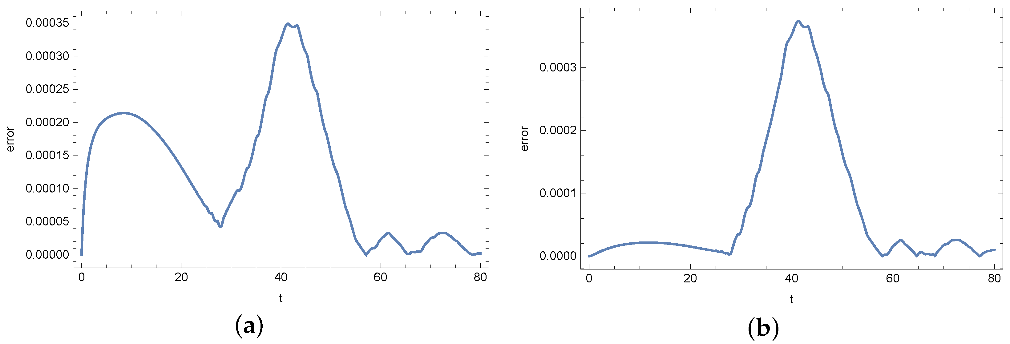
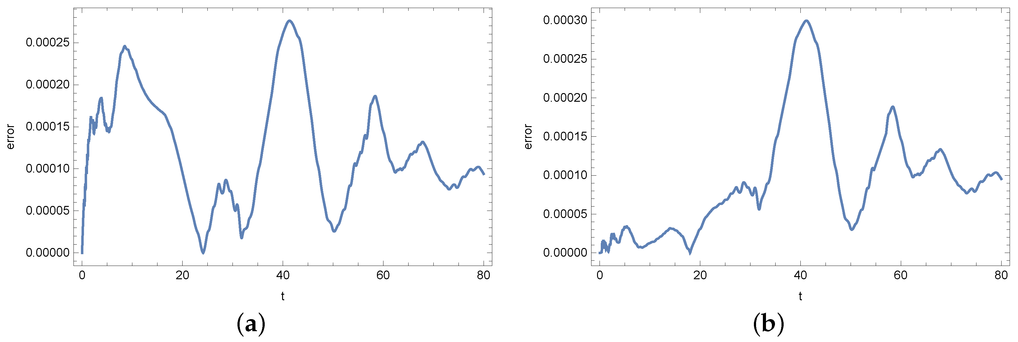
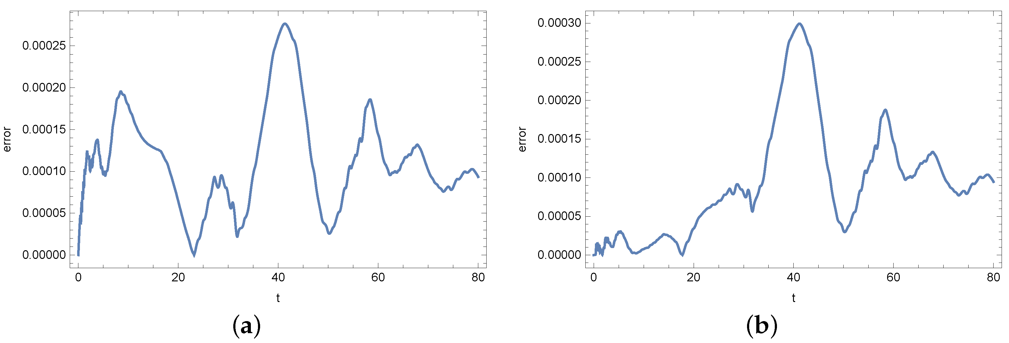
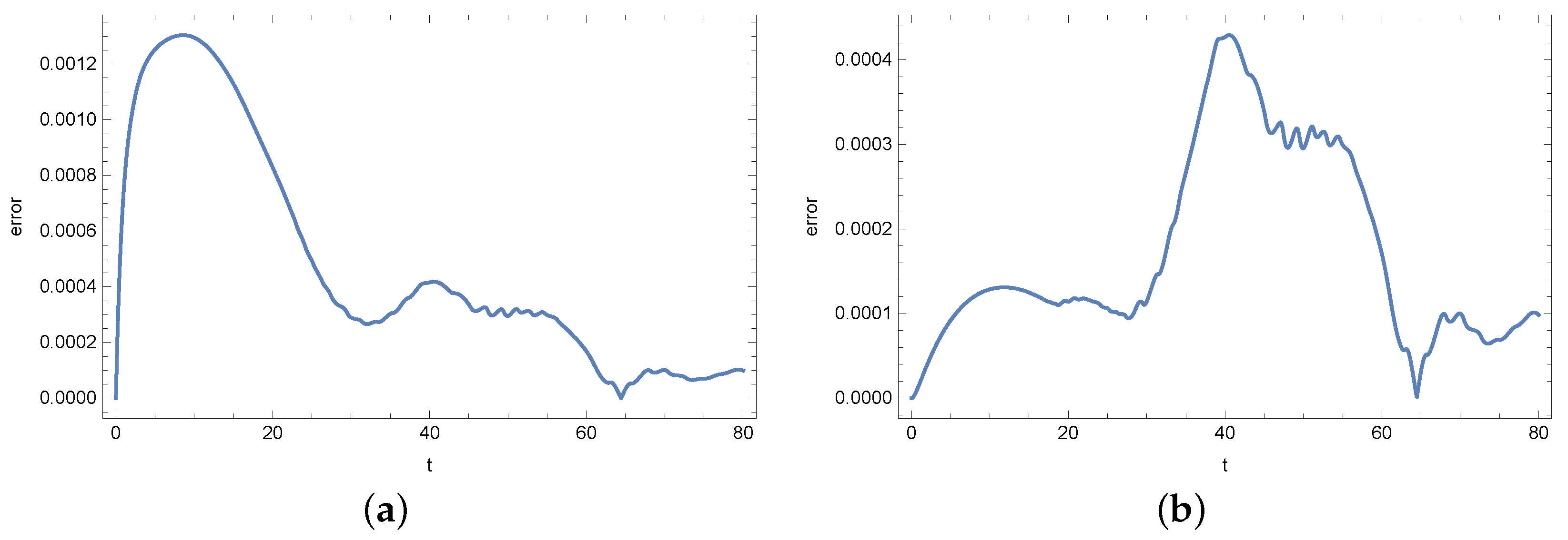
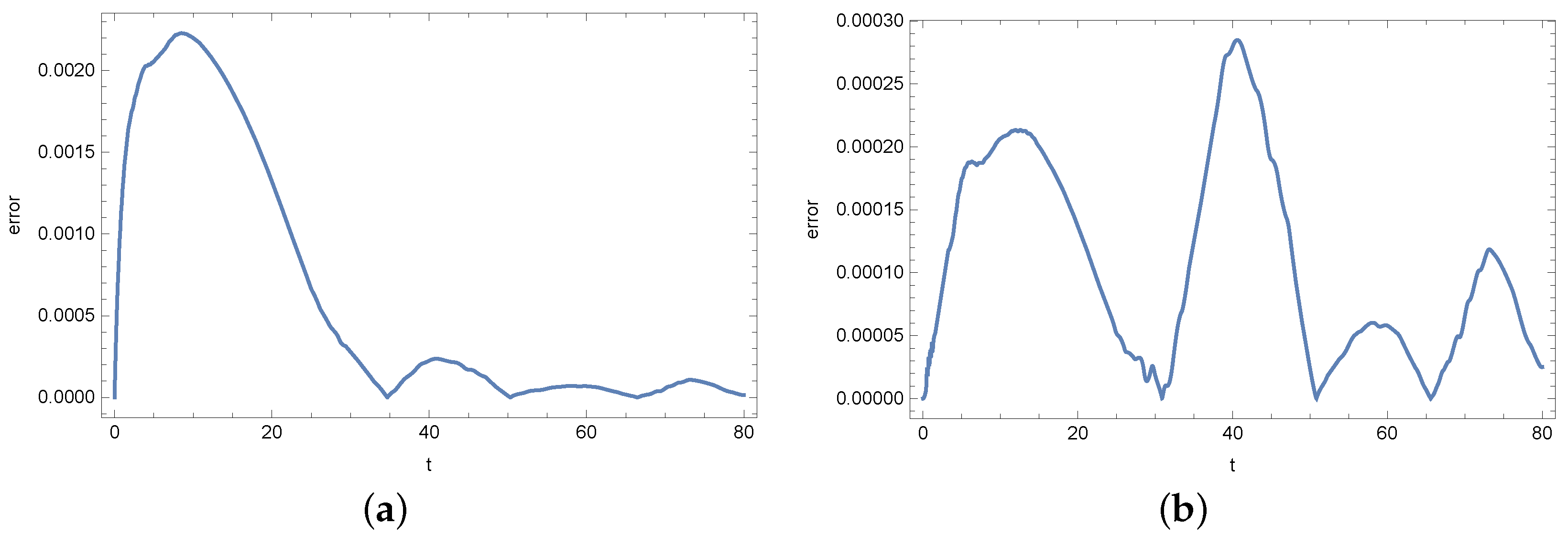
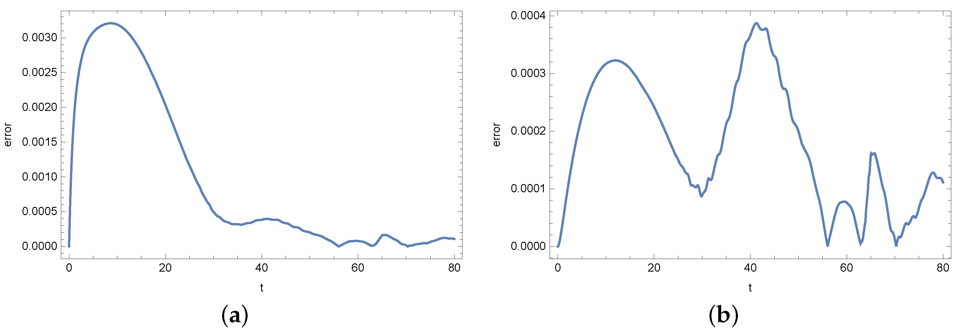
4. Results

In the numerical experiment, input data for the inverse problem have been obtained by solving a direct problem. To prepare the input data, a mesh consisting of 986 finite elements was used. In the calculations necessary to solve the inverse problem, a mesh composed of 602 finite elements was used. This mesh is presented in Figure 3. How changing the mesh affects the values of bacterial density b and substrate concentration s is presented in Figure 4 and Figure 5. The error plot looks similar at two different points of the region. The reason for using a different mesh to generate the input data and a different mesh for solving the inverse problem is related to avoiding the inverse crime [20,21].

The calculations are performed in the region $\mathrm{\Omega }=\left\{\right(x,y),x\in (-4,4),y\in (-4,4\left)\right\}$ and for $t\in [0,80]$. Following parameters are assumed [31]: $v=2.0$, $D_s=1$, $k=0.1$, $v_0=1.5$ and $b_0(x,y)=a_{0}exp\left(\frac{-x^2-y^2}{a}\right)$, where $a=6.25$ and $a_0=0.5$. The exact value of the diffusion coefficient is $D=0.5$. The contour plots of the b (density of active bacteria) and s (concentration of substrate) functions for $t=20$ are shown in Figure 6.

Region $\mathrm{\Omega }$ contains one measuring point, while the measurements are taken every 1 s. The calculations are taken for different positions of the measuring point: $(0,0)$, $(0.5,0.5)$, $(4,0)$ and $(4,4)$. The exact and noised input data are used in the calculations. The noise of input data was implemented in such a way that a random value from $[-\frac{p{b}_e}{100},\frac{p{b}_e}{100}]$ was added to the exact value of $b_e$, where p was the percent disturbance level. The random values are uniformly distributed. Perturbations of $0.5\%$, $1\%$, $2\%$, $5\%$ and $10\%$ were used in the calculations. The exact input data and their noises are shown in Figure 7.

To find the minimum of the objective function J (12) the Fibonacci algorithm was used, which is described in Section 3. The diffusion coefficient D was searched in $(0,1]$ interval with a precision of ${10}^{-7}$.

Figure 8 and Figure 9 present plots of the objective function J in the case of exact input data and $10\%$ noised input data. As we can see in Figure 8 and Figure 9, for small values (≤0.2) of the diffusion coefficient D, the values of the objective function J are relatively large. The minimum is for $D=0.5$.

In

Table 1. Result of reconstruction diffusion coefficient D for measuring points $(0.5,0.5)$ ($D_r$—reconstructed value, ${\Delta }_D$—absolute error, ${\delta }_D$—percentage relative error, $J\left(D_r\right)$—value of objective function).

	${\mathit{D}}_{\mathit{r}}$	${{\Delta }}_{\mathit{D}}$	${\mathit{\delta }}_{\mathit{D}}$ [%]	$\mathit{J}\left({\mathit{D}}_{\mathit{r}}\right)$
0%	$0.498745$	$1.25463\times {10}^{-3}$	$0.25093$	$5.92104\times {10}^{-6}$
$0.5$%	$0.501232$	$1.23154\times {10}^{-3}$	$0.24631$	$9.76260\times {10}^{-4}$
1%	$0.500935$	$9.34980\times {10}^{-4}$	$0.18700$	$3.72183\times {10}^{-3}$
2%	$0.492409$	$7.59105\times {10}^{-3}$	$1.51821$	$1.80198\times {10}^{-2}$
5%	$0.513011$	$1.30115\times {10}^{-2}$	$2.60229$	$9.91133\times {10}^{-2}$
10%	$0.481519$	$1.84813\times {10}^{-2}$	$3.69626$	$3.38221\times {10}^{-1}$

and

Table 2. Result of reconstruction diffusion coefficient D for measuring points $(4,4)$ ($D_r$—reconstructed value, ${\Delta }_D$—absolute error, ${\delta }_D$—percentage relative error, $J\left(D_r\right)$—value of objective function).

	${\mathit{D}}_{\mathit{r}}$	${{\Delta }}_{\mathit{D}}$	${\mathit{\delta }}_{\mathit{D}}$ [%]	$\mathit{J}\left({\mathit{D}}_{\mathit{r}}\right)$
0%	$0.500749$	$7.49011\times {10}^{-4}$	$0.14980$	$3.64599\times {10}^{-5}$
$0.5$%	$0.502123$	$2.12259\times {10}^{-3}$	$0.42452$	$1.05587\times {10}^{-3}$
1%	$0.495409$	$4.59132\times {10}^{-3}$	$0.91826$	$3.36342\times {10}^{-3}$
2%	$0.493628$	$6.37232\times {10}^{-3}$	$1.27446$	$1.64222\times {10}^{-2}$
5%	$0.502123$	$2.12259\times {10}^{-3}$	$0.42451$	$9.19305\times {10}^{-2}$
10%	$0.490746$	$9.25410\times {10}^{-3}$	$1.85082$	$3.23392\times {10}^{-1}$

are presented reconstructed values of coefficient D in the case of calculations for measurement point $(0.5,0.5)$ and $(4,4)$. In the case of noised input data, the percentage error of reconstruction is smaller than the noisy input data. Even for $p=10\%$, the error of reconstruction is less than $3.7\%$ which is satisfying. In the case of calculations for the remaining measuring points, the D coefficient is also reconstructed very well.

Table 3. Errors of reconstruction b and s in measurement point $(0.5,0.5)$ ($\Delta$—absolute error, $\delta$—percentage relative error).

	${{\Delta }}_{\mathit{b}}$	${\mathit{\delta }}_{\mathit{b}}$ [%]	${{\Delta }}_{\mathit{s}}$	${\mathit{\delta }}_{\mathit{s}}$ [%]
0%	$1.77444\times {10}^{-5}$	$1.35385\times {10}^{-2}$	$1.5003\times {10}^{-5}$	$1.63783\times {10}^{-2}$
$0.5$%	$1.55925\times {10}^{-5}$	$1.18967\times {10}^{-2}$	$1.32981\times {10}^{-5}$	$1.45171\times {10}^{-2}$
1%	$1.42339\times {10}^{-5}$	$1.08601\times {10}^{-2}$	$1.32816\times {10}^{-5}$	$1.44991\times {10}^{-2}$
2%	$6.99296\times {10}^{-5}$	$5.33545\times {10}^{-2}$	$2.2793\times {10}^{-5}$	$2.48823\times {10}^{-2}$
5%	$1.09808\times {10}^{-4}$	$8.37807\times {10}^{-2}$	$1.47364\times {10}^{-5}$	$1.60872\times {10}^{-2}$
10%	$1.63983\times {10}^{-4}$	$1.25115\times {10}^{-1}$	$2.31277\times {10}^{-5}$	$2.52477\times {10}^{-2}$

presents errors of reconstruction functions b (density of active bacteria) and s (concentration of substrate) in measurement point $(0.5,0.5)$. In all cases, these errors are minimal and do not exceed $0.13\%$. A similar situation occurs in the case of identification of the functions b and s in the entire region $\mathrm{\Omega }$ (see

Table 4. Errors of reconstruction b and s in entire region in the case of calculations for measurement point $(0.5,0.5)$ ($\Delta$—absolute error, $\delta$—percentage relative error).

	${{\Delta }}_{\mathit{b}}$	${\mathit{\delta }}_{\mathit{b}}$ [%]	${{\Delta }}_{\mathit{s}}$	${\mathit{\delta }}_{\mathit{s}}$ [%]
0%	$3.44446\times {10}^{-7}$	$2.14275\times {10}^{-2}$	$1.84832\times {10}^{-7}$	$1.62498\times {10}^{-2}$
$0.5$%	$2.76896\times {10}^{-7}$	$1.72253\times {10}^{-2}$	$1.65205\times {10}^{-7}$	$1.45242\times {10}^{-2}$
1%	$2.70628\times {10}^{-7}$	$1.68353\times {10}^{-2}$	$1.64835\times {10}^{-7}$	$1.44917\times {10}^{-2}$
2%	$6.26896\times {10}^{-7}$	$3.89982\times {10}^{-2}$	$2.69966\times {10}^{-7}$	$2.37345\times {10}^{-2}$
5%	$9.48329\times {10}^{-7}$	$5.89941\times {10}^{-2}$	$1.56614\times {10}^{-7}$	$1.3769\times {10}^{-2}$
10%	$1.42314\times {10}^{-6}$	$8.85313\times {10}^{-2}$	$2.33235\times {10}^{-7}$	$2.05052\times {10}^{-2}$

). Even in case of $10\%$ noised input data, relative errors of reconstruction b and s are equal to $8.86\times {10}^{-2}\%$ and $2.06\%$, respectively. In the case of calculations for the remaining measurement points, similar results were obtained. This is illustrated by Figure 10, which shows the mean errors of identifying the b and s functions obtained during the calculations for various measurement points and selected noises of the input data. Each time, the values of both functions in the measuring point are estimated very well. The identification errors are much smaller than the input errors. They slightly depend on the location of the measurement point. The b function reconstruction error is slightly greater than in the case of the s function. In the case of the b function, the biggest error occurred for the $(0,0)$ measurement point and the 5% disturbance of the input data and this error is equal to $0.282$%. On the other hand, in the case of the s function, the largest error occurred for the $\left(4.0\right)$ measurement point and 10% disturbance and is equal to $0.076$%. Plots of reconstructed density of active bacteria b and concentration of substrate s in measurement point $(0.5,0.5)$ and $(4,4)$ for input data noised by 10% error are presented in Figure 11.

Figure 12 presents the mean relative errors of reconstructing the functions b and s in the entire considered area obtained during calculations for various measurement points and selected disturbances of the input data. Furthermore, the obtained errors for the entire area are much smaller than the input data errors. Changing the position of the measuring point has a small effect on the obtained errors. In all cases, errors are very small. In the case of the b function, the largest error is noted for $(0,0)$ and 5% disturbances and it is equal to $0.185$%. In turn, in the case of the s function, the largest error occurred for the point $\left(4.0\right)$ and 10% disturbances and it is equal to to $0.077$%.

At the end of this section, we present Figure 13, Figure 14, Figure 15, Figure 16, Figure 17 and Figure 18 showing the errors of the reconstruction of functions b and s in measurement points for different noises of the input data. In the case of the density of active bacteria (function b) and low input data noise ($p=0\%,0.5\%,1\%$), the greatest errors are noted around the time t = 40 s, while for the input data noised by $p=2\%,5\%,10\%$ the highest value of error is around t = 10 s. In the case of the concentration of substrate, the highest error is around t = 40 s for all input data.

5. Conclusions

The model presented in the paper describes the distribution of active bacteria (function b) and the concentration of the substrate (function s) in space and time. For solving a system of differential equations with initial-boundary conditions, the finite element method was used. In modeling various types of phenomena, it is sometimes necessary to determine some model parameters that are difficult to measure by sensors. To determine these parameters is needed to solve the inverse problem. A method of solving the inverse problem, consisting in determining the diffusion coefficient of active bacteria based on measurements of the density of bacteria at a fixed point of the region, is presented. The considered method, based on the minimization of the objective function with the Fibonacci algorithm, gives good results. Even for noisy input data, the errors are at a satisfactory level. The errors of reconstruction of the b and s functions, in all cases, are less than $0.3\%$, while the error of diffusion coefficient D does not exceed the noise of input data. Furthermore, changing the location of the measurement point does not have a large impact on the obtained results. The method was implemented in the Wolfram language, and the calculations were performed in the Mathematica 12.3 platform. The computation time for the inverse problem was about $130$ s. This time can be shortened by using more advanced Wolfram statements or implementing it in another language. The obtained results confirm the accuracy and stability of the presented method.

References

- Xiong, L.; Cao, Y.; Cooper, R.; Rappel, W.-J.; Hasty, J.; Tsimring, L. Flower-like patterns in multi-species bacterial colonies. eLIFE 2020, 9, e48885. [Google Scholar] [CrossRef]
- Rhodeland, B.; Hoeger, K.; Ursell, T. Bacterial surface motility is modulated by colony-scale flow and granular jamming. J. R. Soc. Interface 2020, 17, 20200147. [Google Scholar] [CrossRef] [PubMed]
- Matoz-Fernandez, D.; Arnaouteli, S.; Porter, M.; MacPhee, C.E.; Stanley-Wall, N.R.; Davidson, F.A. Comment on ”Rivalry in Bacillus subtilis colonies: Enemy or family?”. Soft Matter 2020, 16, 3344–3346. [Google Scholar] [CrossRef] [PubMed]
- Brzozowski, R.S.; Tomlinson, B.R.; Sacco, M.D.; Chen, J.J.; Ali, A.N.; Chen, Y.; Shaw, L.N.; Eswaraa, P.J. Interdependent YpsA- and YfhS-Mediated Cell Division and Cell Size Phenotypes in Bacillus subtilis. mSphere 2020, 5, e00655-20. [Google Scholar] [CrossRef] [PubMed]
- Hernandez-Valdes, J.A.; Zhou, L.; de Vries, M.P.; Kuipers, O.P. Impact of spatial proximity on territoriality among human skin bacteria. NPJ Biofilms Microbiomes 2020, 6, 30. [Google Scholar] [CrossRef] [PubMed]
- Sui, Z.-W.; Wang, B.; Liu, S.-Y.; Wang, J.; Fu, B.-Q.; Zhuo, T.-Y.; Wang, Y. Study on Measurement Method of Bacillus subtilis var. niger Spore. Jiliang Xuebao/Acta Metrol. Sin. 2020, 41, 1171–1176. [Google Scholar]
- Earl, C.; Arnaouteli, S.; Bamford, N.C.; Porter, M.; Sukhodub, T.; MacPhee, C.E.; Stanley-Wall, N.R. The majority of the matrix protein TapA is dispensable for Bacillus subtilis colony biofilm architecture. Mol. Microbiol. 2020. [Google Scholar] [CrossRef]
- Schwarcz, D.; Levine, H.; Ben-Jacob, E.; Ariel, G. Uniform modeling of bacterial colony patterns with varying nutrient and substrate. Phys. D 2016, 318–319, 91–99. [Google Scholar] [CrossRef]
- Miyata, S.; Sasaki, T. Asymptotic analysis of a chemotactic model of bacteria colonies. Math. Biosci. 2006, 201, 184–194. [Google Scholar] [CrossRef]
- Golding, I.; Kozlovsky, Y.; Cohen, I.; Ben-Jacob, E. Studies of bacterial branching growth using reaction-diffusion models for colonial development. Phys. A 1998, 260, 510–554. [Google Scholar] [CrossRef]
- Shimada, H.; Ikeda, T.; Wakita, J.; Itoh, H.; Kurosu, S.; Hiramatsu, F.; Nakatsuchi, M.; Yamazaki, Y.; Matsuyama, T.; Matsushita, M. Dependence of local cell density on concentric ring colony formation by bacterial species bacillus subtilis. J. Phys. Soc. Jpn. 2003, 73, 1082–1089. [Google Scholar] [CrossRef]
- Brociek, R.; Słota, D.; Król, M.; Matula, G.; Kwaśny, W. Comparison of mathematical models with fractional derivative for the heat conduction inverse problem based on the measurements of temperature in porous aluminum. Int. J. Heat Mass Transf. 2019, 143, 118440. [Google Scholar] [CrossRef]
- Brociek, R.; Słota, D.; Król, M.; Matula, G.; Kwaśny, W. Modeling of heat distribution in porous aluminum using fractional differential equation. Fractal Fract. 2017, 1, 17. [Google Scholar] [CrossRef]
- Shang, Z.; Liao, Z.; Sarasua, J.A.; Billingham, J.; Axinte, D. On modelling of laser assisted machining: Forward and inverse problems for heat placement control. Int. J. Mach. Tools Manuf. 2019, 138, 36–50. [Google Scholar] [CrossRef]
- Kefai, A.; Yildiz, M. Modeling of sensor placement strategy for shape sensing and structural health monitoring of a wing-shaped sandwich panel using inverse finite element method. Sensors 2017, 17, 2775. [Google Scholar]
- Liang, D.; Cheng, J.; Ke, Z.; Ying, L. Deep magnetic resonance image reconstruction: Inverse problems meet neural networks. IEEE Signal Process. Mag. 2020, 37, 141–151. [Google Scholar] [CrossRef]
- Brociek, R.; Hetmaniok, E.; Słota, D. Reconstruction of aerothermal heating for the thermal protection system of a reusable launch vehicle. Appl. Therm. Eng. 2023, 219, 119405. [Google Scholar] [CrossRef]
- Brociek, R.; Hetmaniok, E.; Napoli, C.; Capizzi, G.; Słota, D. Estimation of aerothermal heating for a thermal protection system with temperature dependent material properties. Int. J. Therm. Sci. 2023, 188, 108229. [Google Scholar] [CrossRef]
- Smyl, D.; Liu, D. Less is often more: Applied inverse problems using hp-forward models. J. Comput. Phys. 2019, 399, 108949. [Google Scholar] [CrossRef]
- Kaipio, J.; Somersalo, E. Statistical and Computational Inverse Problems; Springer: New York, NY, USA, 2005. [Google Scholar]
- Kaipio, J.; Somersalo, E. Statistical inverse problems: Discretization, model reduction and inverse crimes. J. Comput. Appl. Math. 2007, 198, 493–504. [Google Scholar] [CrossRef]
- Clermont, G.; Zenker, S. The inverse problem in mathematical biology. Math. Biosci. 2015, 260, 11–15. [Google Scholar] [CrossRef] [PubMed]
- Abdulla, U.G.; Poteau, R. Identification of parameters in systems biology. Math. Biosci. 2018, 305, 133–145. [Google Scholar] [CrossRef] [PubMed]
- Capasso, V.; Kunze, H.E.; La Torre, D.; Vrscay, E.R. Solving inverse problems for biological models using the collage method for differential equations. J. Math. Biol. 2013, 67, 25–38. [Google Scholar] [CrossRef] [PubMed]
- Kabanikhin, S.I.; Krivorotko, O.I. Optimization methods for solving inverse immunology and epidemiology problems. Comput. Math. Math. Phys. 2020, 60, 580–589. [Google Scholar] [CrossRef]
- Doumic, M.; Maia, P.; Zubelli, J.P. On the calibration of a size-structured population model from experimental data. Acta Biotheor. 2010, 58, 405–413. [Google Scholar] [CrossRef]
- Barnsley, M.F. Fractals Everywhere; AP Professional: Boston, MA, USA, 2012. [Google Scholar]
- Bao, W.; Yang, B.; Chen, B. 2-hydr_Ensemble: Lysine 2-hydroxyisobutyrylation identification with ensemble method. Chemom. Intell. Lab. Syst. 2021, 215, 104351. [Google Scholar] [CrossRef]
- Yang, B.; Bao, W.; Wang, J. Active disease-related compound identification based on capsule network. Briefings Bioinform. 2022, 23, bbab462. [Google Scholar] [CrossRef]
- Bao, W.; Cui, Q.; Chen, B.; Yang, B. Phage_UniR_LGBM: Phage Virion Proteins Classification with UniRep Features and LightGBM Model. Comput. Math. Methods Med. 2022, 2022, 9470683. [Google Scholar] [CrossRef]
- Rida, S.Z.; El-Sayed, A.M.A.; Arafa, A.A.M. Effect of bacterial memory dependent growth by using fractional derivatives reaction-diffusion chemotactic model. J. Stat. Phys. 2010, 140, 797–811. [Google Scholar] [CrossRef]
- Kawasaki, K.; Mochizuki, A.; Matsushita, M.; Umeda, T.; Shigesada, N. Modeling spatio-temporal patterns created by Bacillus subtilis. J. Teor. Biol. 1997, 188, 177–185. [Google Scholar] [CrossRef]
- Gill, P.E.; Murray, W.; Wright, M.H. Practical Optimization; Academic Press: London, UK, 1981. [Google Scholar]
- Mishra, S.K.; Ram, B. Introduction to Unconstrained Optimization with R; Springer Nature: Singapore, 2019. [Google Scholar]
- Wolfram, S. An Elementary Introduction to the Wolfram Language; Wolfram Media: Champaign, IL, USA, 2017. [Google Scholar]