
Detecting Heavy Neutral SUSY Higgs Bosons Decaying to Sparticles at the High-Luminosity LHC

Abstract
1. Introduction
- The superpotential parameter enters Equation (2) directly at tree level, implying that GeV. This means that for heavy Higgs searches with , then SUSY decay modes of should already be open. If these additional decay widths to SUSY particles are substantial, then the heavy Higgs branching ratios to the usually assumed SM search modes will be significantly reduced.
- For , then sets the heavy Higgs mass scale () while sets the mass scale for . Then naturalness requires [23]
2. Production of and followed by Dominant Decay to SUSY Particles
2.1. A Natural SUSY Benchmark Point
Some (Cosmological) Aspects of Our Benchmark (BM) Point
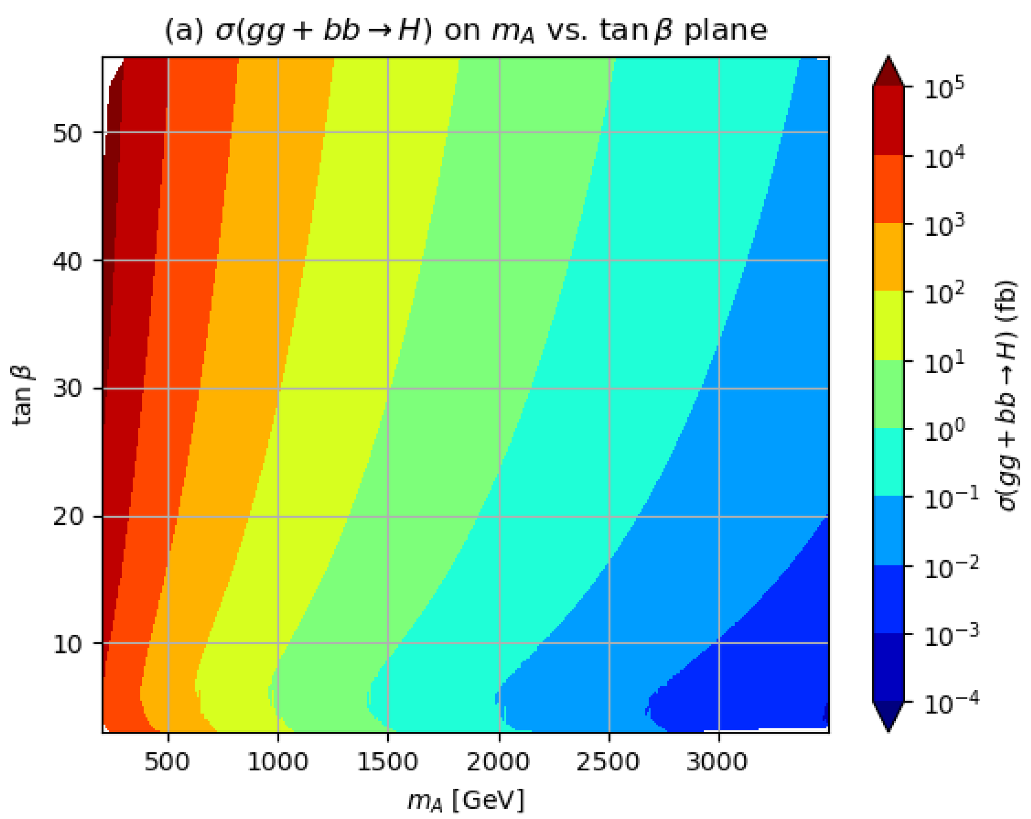
2.2. H and A Production Cross Sections at LHC


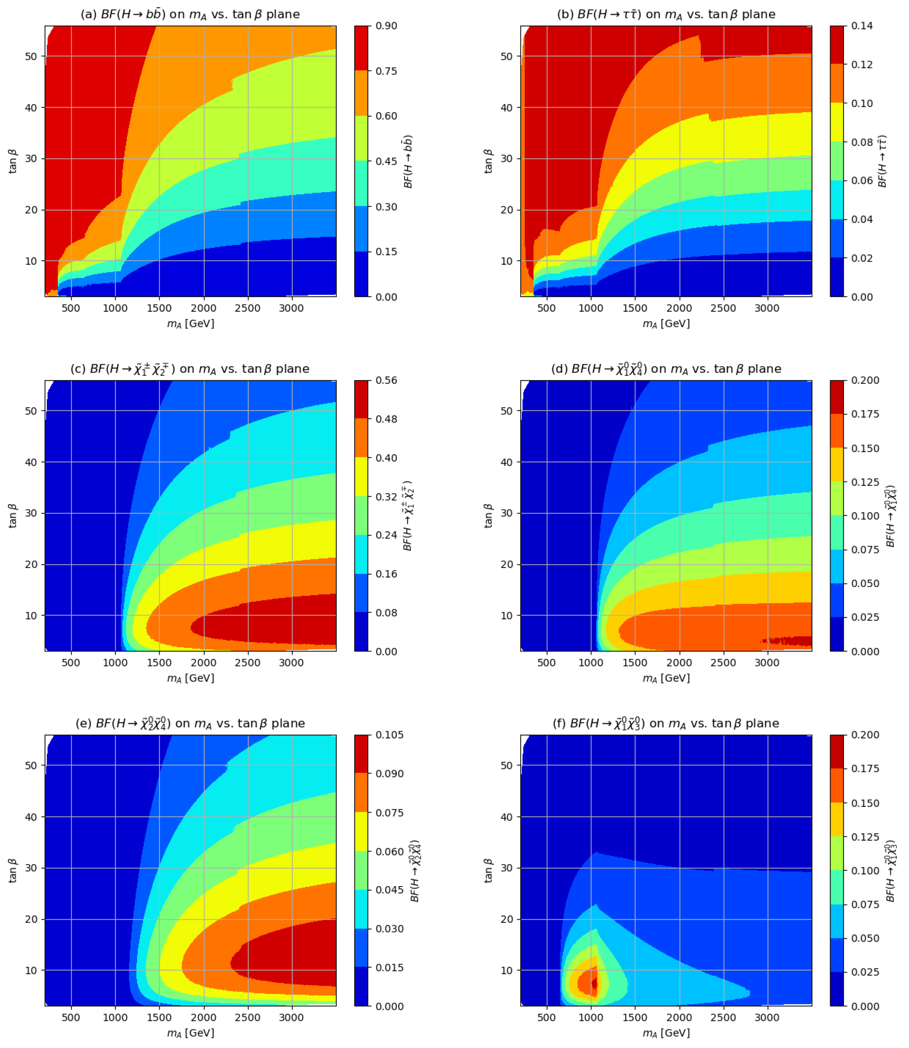
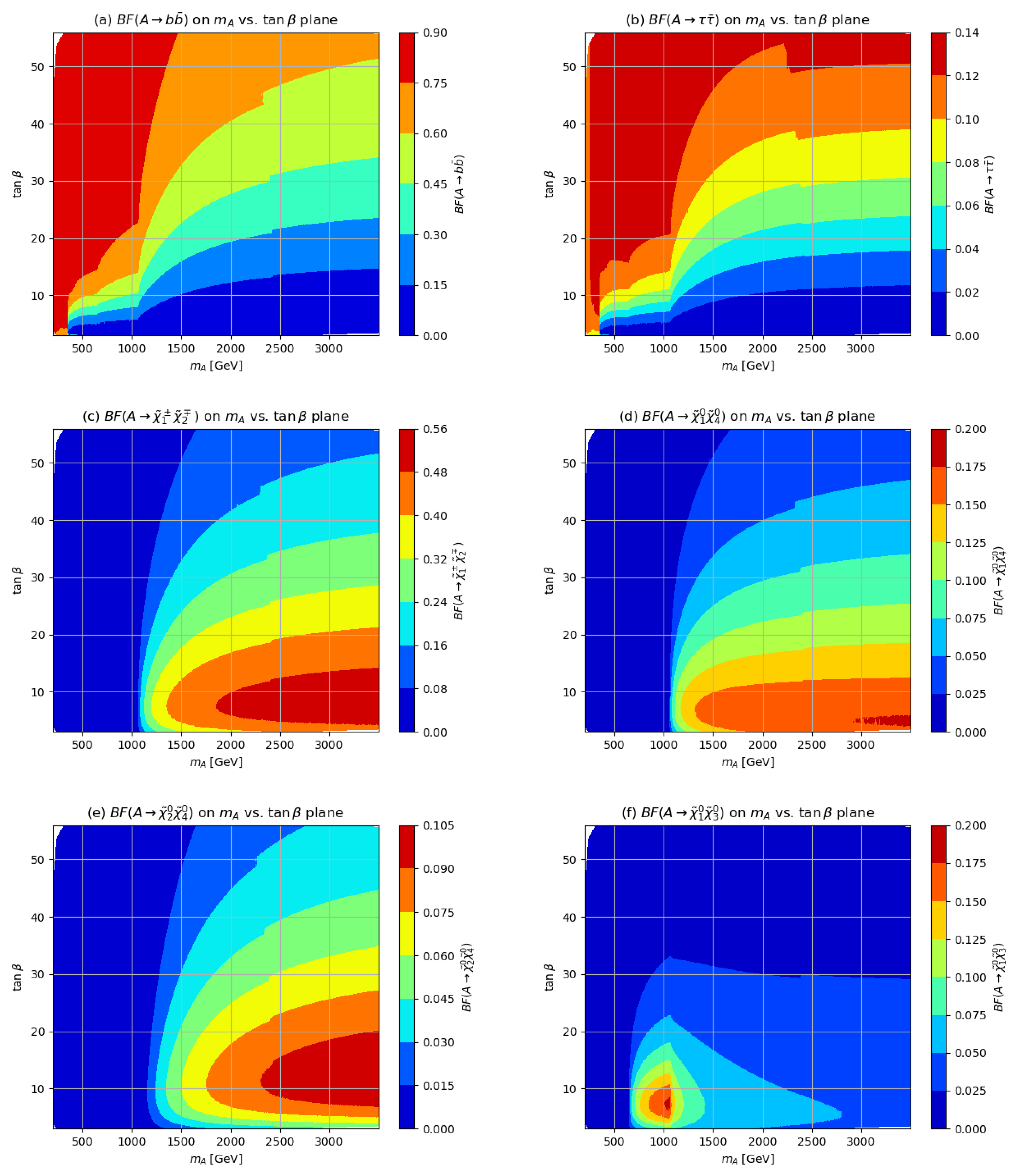
2.3. H and A Branching Fractions
3. A Survey of Various Signal Channels
- ,
- and
- .
- Baseline small-radius jet (SRj): Using anti- jet finder algorithm, require GeV with jet cone size and .
- Baseline large-radius jet (LRj): Using anti- jet finder algorithm, require GeV with jet cone size and , for all signatures except for, for which . The large-radius jets are formed using calorimeter deposits (or track information for muons) so that even isolated leptons (see below) are included as constituents of these jets. This will be especially important for the signal examined in Section 3.4 below.
- Baseline isolated lepton: Satisfy basic Delphes lepton isolation requirement with GeV, lepton cone size , and while , where is defined in Delphes as , for calorimetric cells within the lepton cone.
- SRj: Satisfy above SRj requirement plus .
- b-jets: Satisfy above SRj requirement plus b-jet tagged by Delphes b-tagging requirement.
- Signal leptons: Require above-baseline lepton qualities plus GeV with , while GeV with .
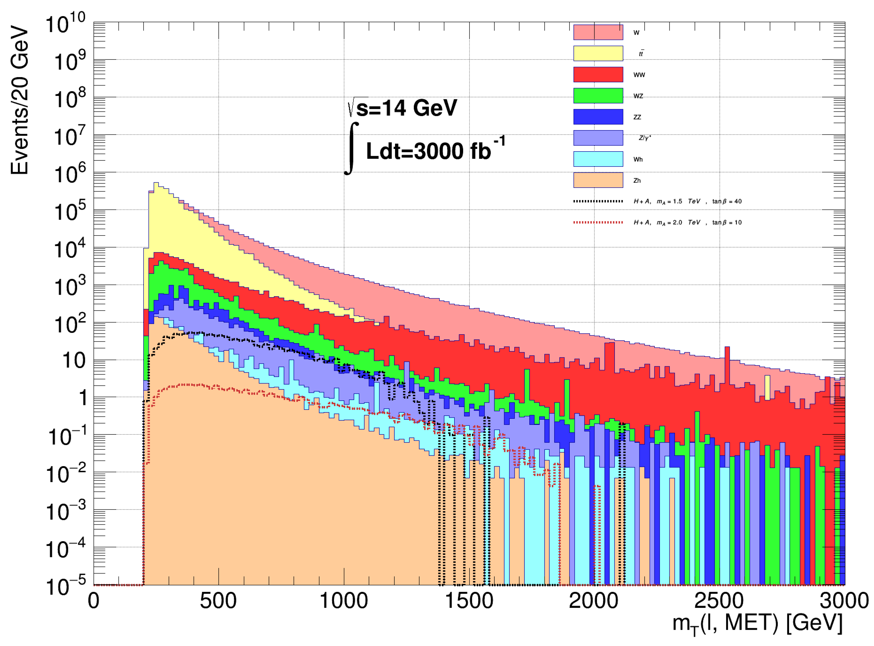
3.1. Signal
- Exactly one baseline lepton (and no LRjs, which will comprise an alternative channel: see below). This lepton should also satisfy signal lepton requirements.
- ;
- GeV;
- ;
- Transverse mass GeV;
- GeV where .
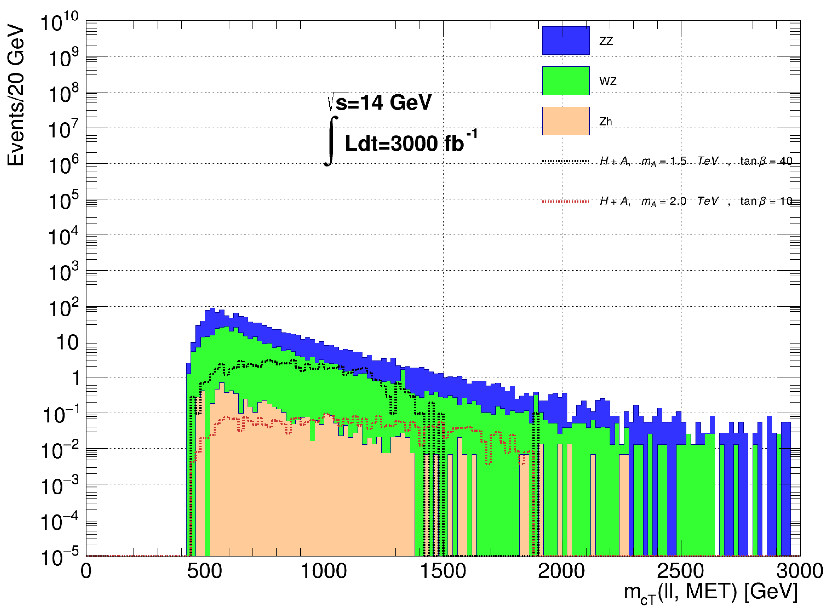
3.2. Signal
- Exactly two baseline leptons (veto additional leptons).
- The two leptons satisfy signal lepton requirements and are opposite-sign/same flavor (OS/SF).
- The dilepton pair invariant mass reconstructs : GeV.
- GeV;
- GeV; where is the azimuthal angle between the and the closest lepton or jet with GeV;
- , () and ;
- ;
- ;
- GeV.
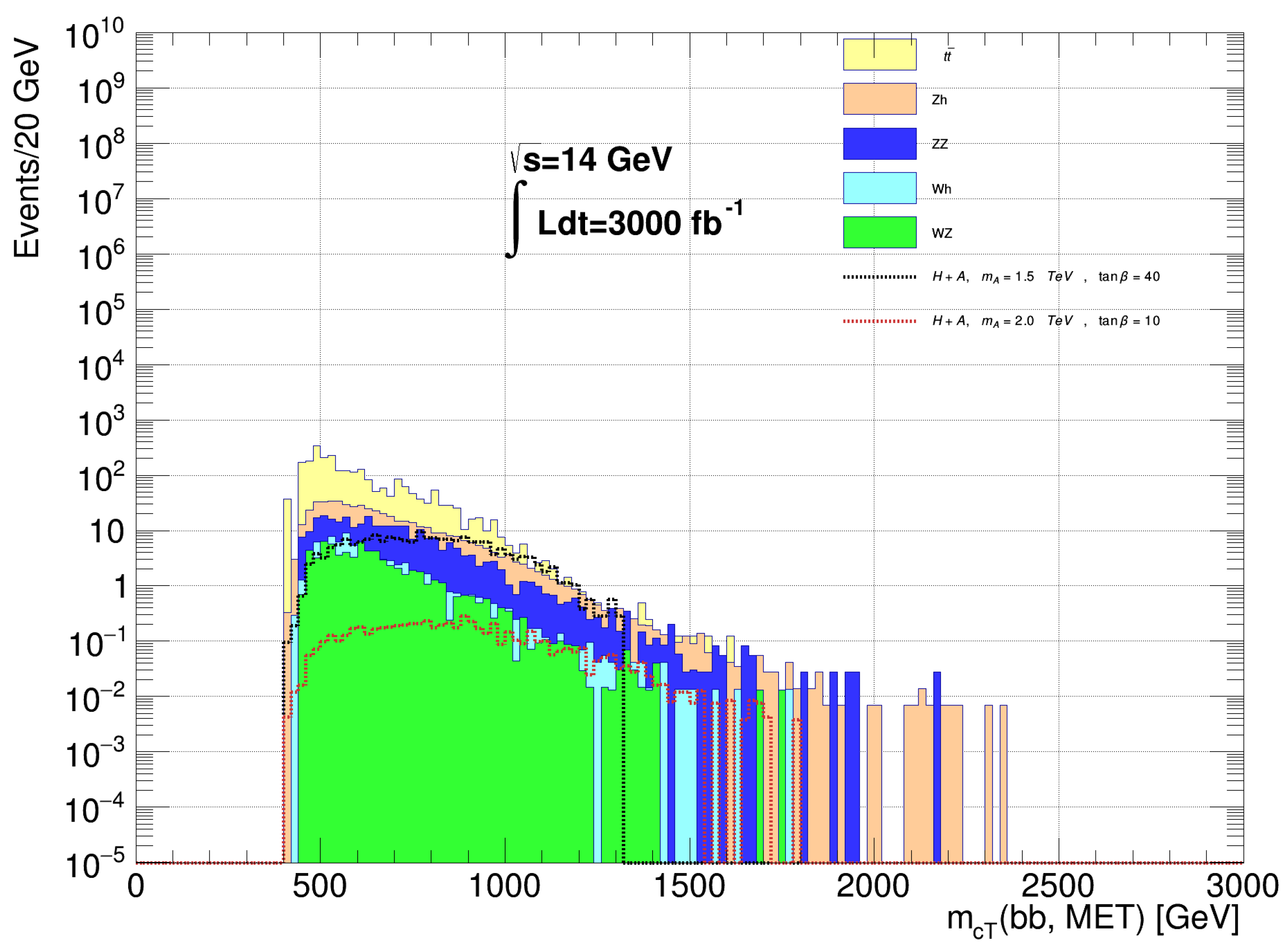
3.3. Signal
- At least two tagged b-jets;
- Veto any baseline leptons;
- Exactly one LRj;
- At least two b-jets within the cone of the LRj;
- Exactly one di-b-jet pair within the cone of the LRj reconstructs the light Higgs mass: GeV;
- GeV.
- GeV;
- GeV;
- GeV;
- GeV;
- ;
- ;
- ;
- ;
- where j loops over all baseline SR jets in the event;
- .
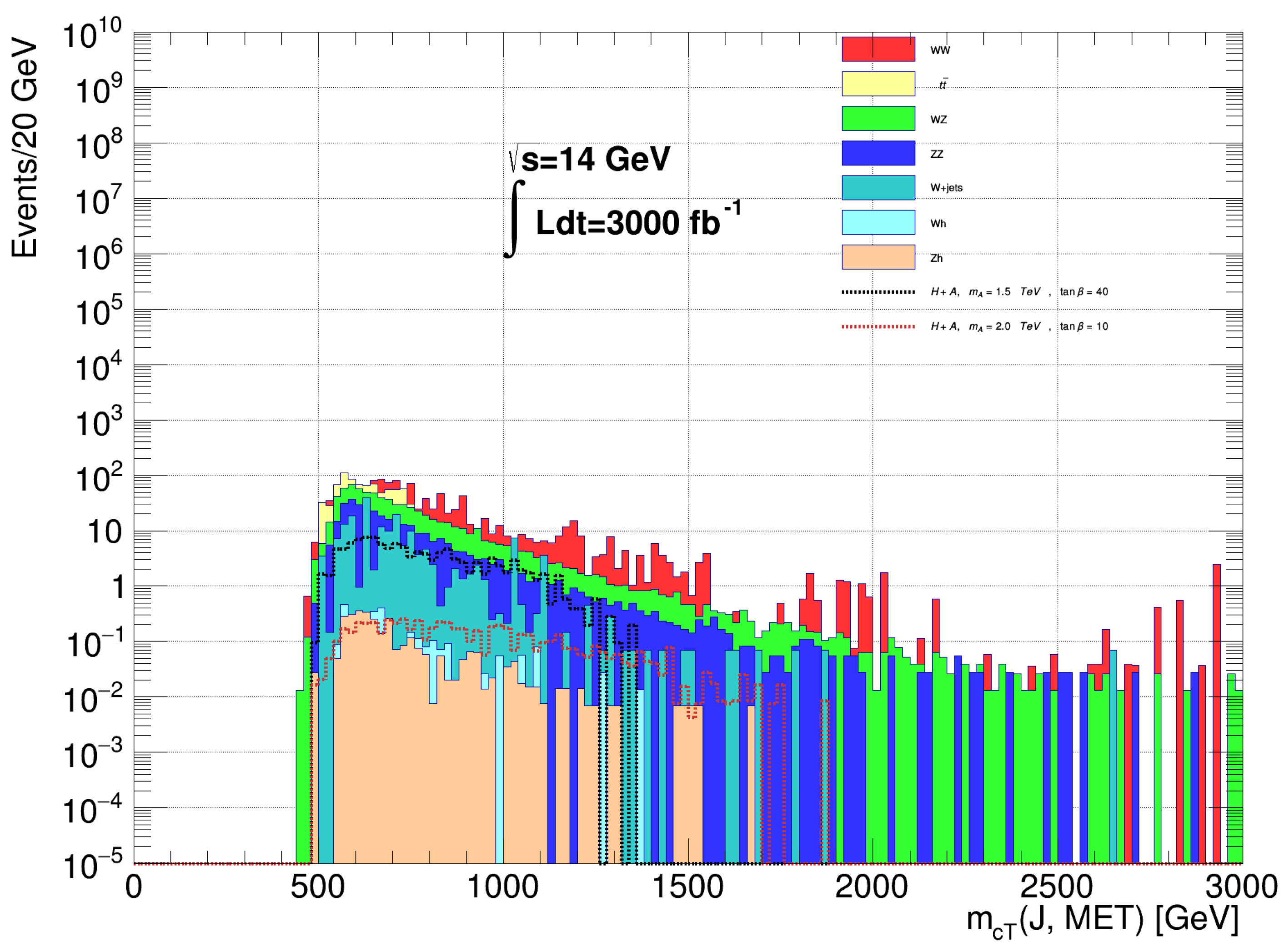
3.4. Signal
- Exactly one signal lepton and no additional baseline leptons in the event.
- Exactly one LRj with invariant mass GeV in accord with a source of either W, Z (or h).
- The lepton is within the cone of the LRj.
- GeV;
- GeV;
- ;
- GeV;
- ;
- ;
- No b-jet within cone of the LRj;
- No jets with GeV outside the cone of the LRj.
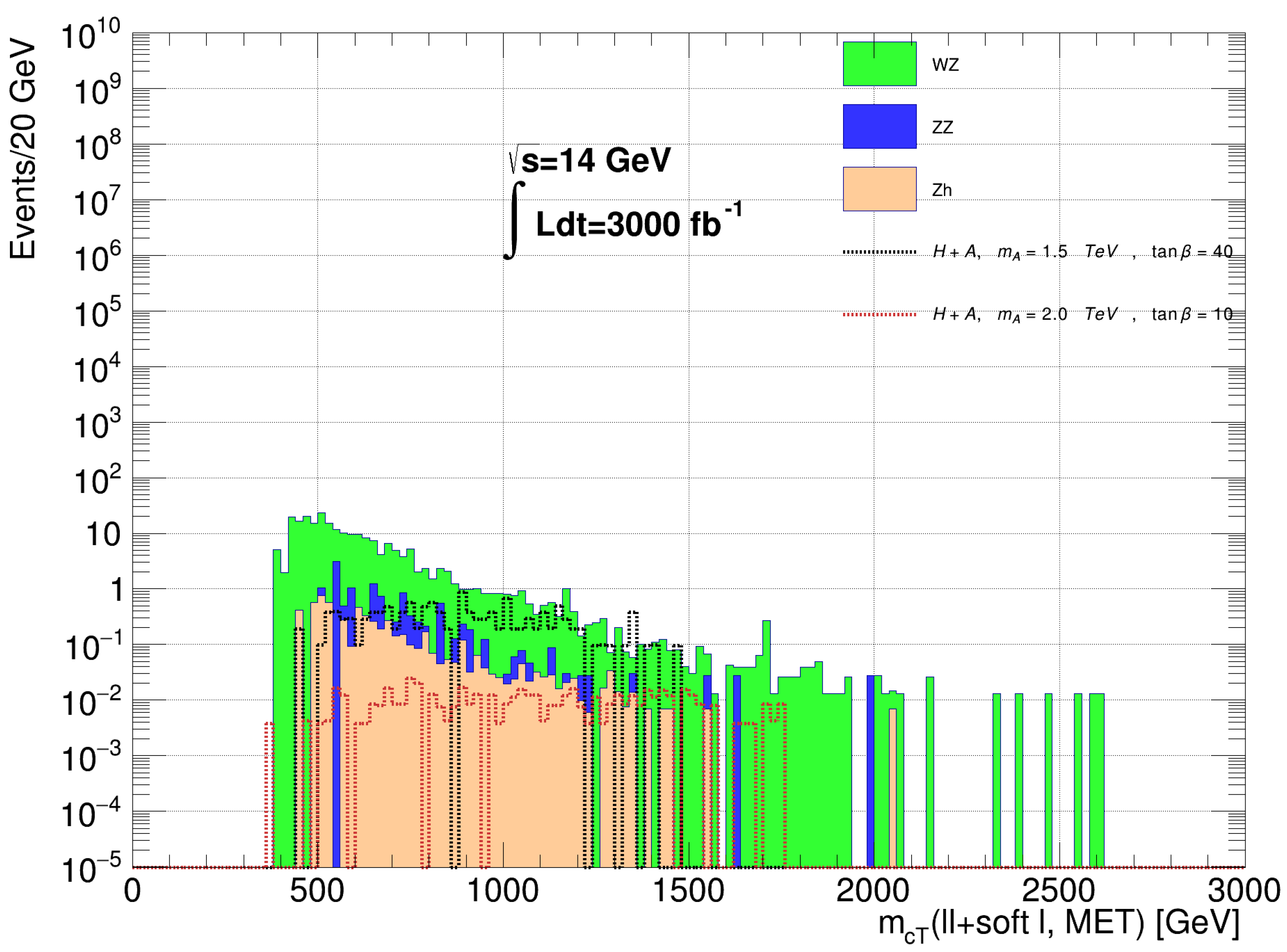
3.5. Signal
- Exactly three baseline leptons.
- At least two leptons satisfy the signal lepton requirement.
- At least two leptons are OS/SF leptons.
- At least one OS/SF pair satisfies the Z-mass requirement: GeV; if more than one pair satisfy the Z-mass, then the pair closest to is chosen whilst the third is designated .
- GeV;
- GeV;
- GeV;
- ; ;
- ;
- ;
- GeV.
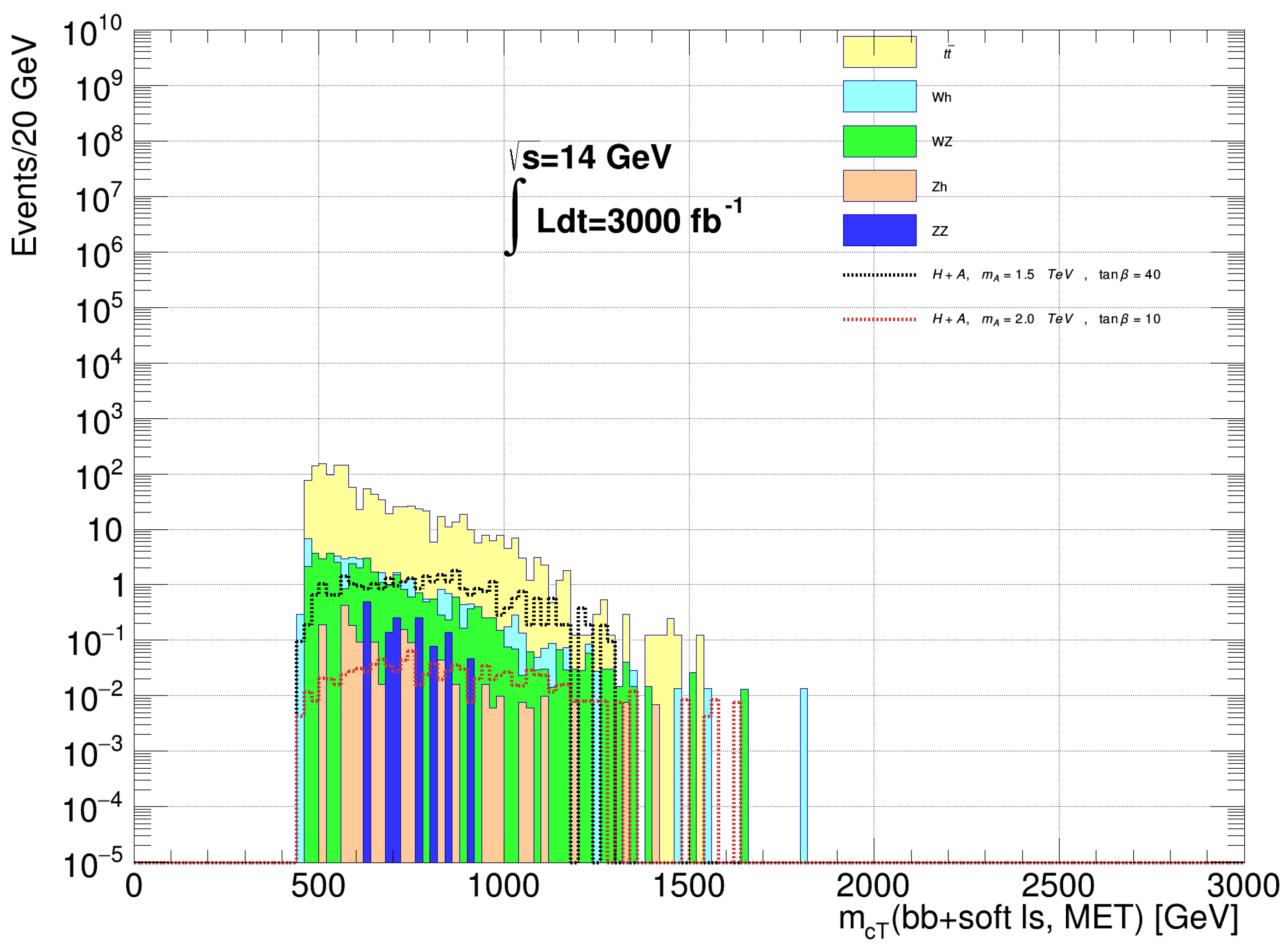
3.6. Signal
- At least two b-jet candidates;
- At least one baseline lepton;
- Exactly one LRj;
- At least two b-jets within the cone of the LRj;
- Exactly one pair of b-jets within the cone of the LRj reconstructs the light Higgs: GeV;
- GeV, and
- .
- GeV;
- GeV;
- GeV for any ℓ in the event;
- GeV;
- ;
- ;
- ;
- , where j cycles over all SR jets in the event, and
- .
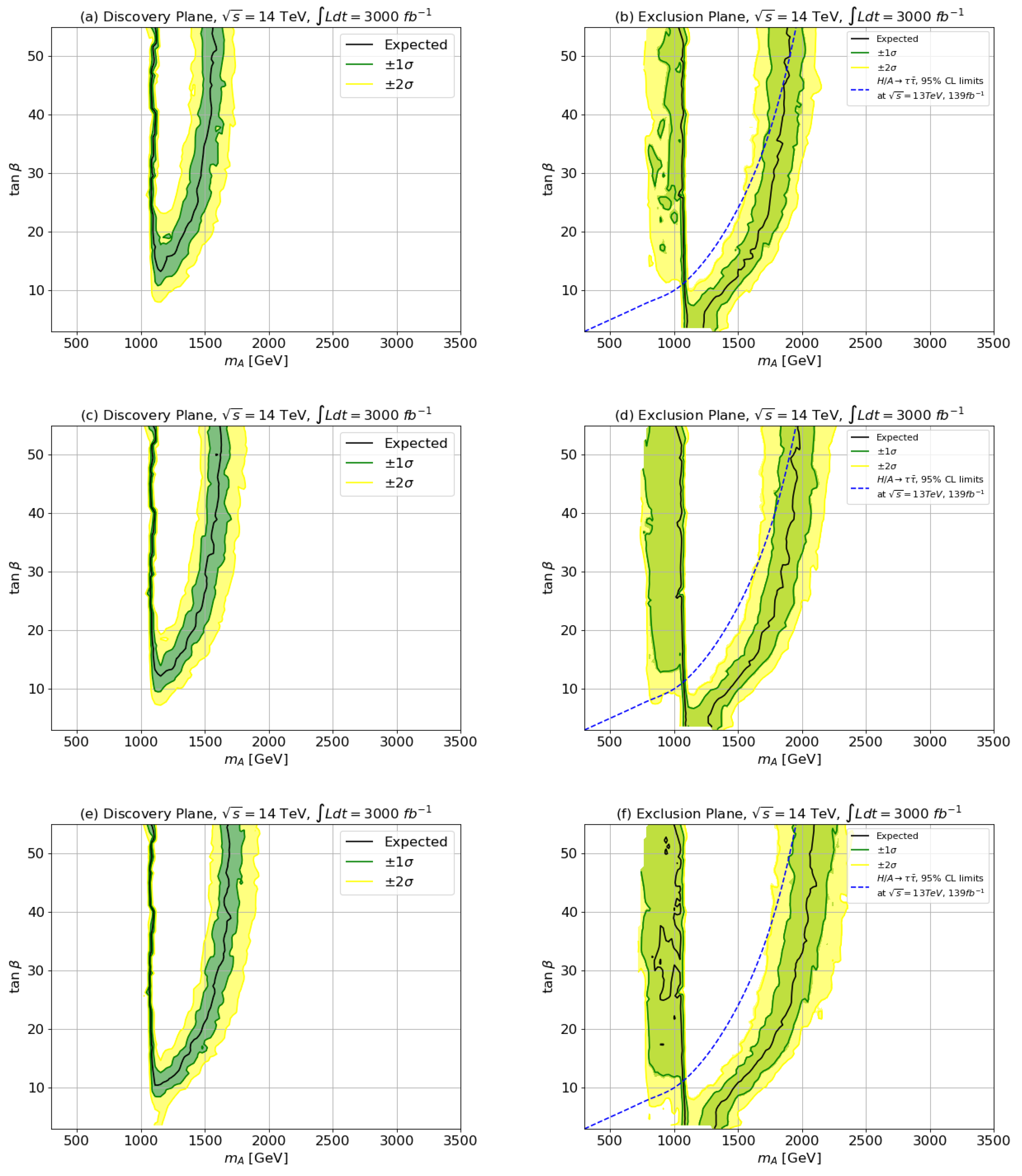
4. Regions of the vs. Plane Accessible to HL-LHC
5. Conclusions
Author Contributions
Funding
Data Availability Statement
Acknowledgments
Conflicts of Interest
References
- Baer, H.; Tata, X. Weak Scale Supersymmetry: From Superfields to Scattering Events; Cambridge University Press: Cambridge, UK, 2006. [Google Scholar]
- Drees, M.; Godbole, R.; Roy, P. Theory and Phenomenology of Sparticles: An Account of Four-Dimensional N = 1 Supersymmetry in High Energy Physics; World Scientific: Singapore, 2004. [Google Scholar]
- Baer, H.; Barger, V.; Salam, S.; Sengupta, D.; Sinha, K. Status of weak scale supersymmetry after LHC Run 2 and ton-scale noble liquid WIMP searches. Eur. Phys. J. Spec. Top. 2020, 229, 3085–3141. [Google Scholar] [CrossRef]
- Cadamuro, L. Higgs boson couplings and properties. PoS LHCP 2019, 2019, 101. [Google Scholar] [CrossRef][Green Version]
- Gunion, J.F.; Haber, H.E. The CP conserving two Higgs doublet model: The Approach to the decoupling limit. Phys. Rev. D 2003, 67, 075019. [Google Scholar] [CrossRef]
- Craig, N.; Galloway, J.; Thomas, S. Searching for Signs of the Second Higgs Doublet. arXiv 2013, arXiv:1305.2424. [Google Scholar]
- Carena, M.; Low, I.; Shah, N.R.; Wagner, C.E.M. Impersonating the Standard Model Higgs Boson: Alignment without Decoupling. JHEP 2014, 4, 15. [Google Scholar] [CrossRef]
- Aad, G.; Abbott, B.; Abbott, D.C.; Abbott, A.; Abed Abud, K.; Abeling, D.K.; Abhayasinghe, S.H.; Abidi, O.S.; AbouZeid, N.L.; Abraham, H.; et al. Search for heavy Higgs bosons decaying into two tau leptons with the ATLAS detector using pp collisions at =13 TeV. Phys. Rev. Lett. 2020, 125, 051801. [Google Scholar] [CrossRef]
- CMS Collaboration. Searches for additional Higgs bosons and for vector leptoquarks in ττ final states in proton-proton collisions at = 13 TeV. arXiv 2022, arXiv:2208.02717. [Google Scholar]
- Bagnaschi, E.; Bahl, H.; Fuchs, E.; Hahn, T.; Heinemeyer, S.; Liebler, S.; Patel, S.; Slavich, P.; Stefaniak, T.; Wagner, C.E.M.; et al. MSSM Higgs Boson Searches at the LHC: Benchmark Scenarios for Run 2 and Beyond. Eur. Phys. J. C 2019, 79, 617. [Google Scholar] [CrossRef]
- ATLAS Collaboration. Search for squarks and gluinos in final states with jets and missing transverse momentum using 139 fb−1 of = 13 TeV pp collision data with the ATLAS detector. JHEP 2021, 2, 143. [Google Scholar] [CrossRef]
- Sirunyan, A.M.; Tumasyan, A.; Adam, W.; Ambrogi, F.; Bergauer, T.; Brandstetter, J.; Dragicevic, M.; Erö, J.; Valle, A.E.D.; Flechl, M.; et al. Search for supersymmetry in proton-proton collisions at 13 TeV in final states with jets and missing transverse momentum. JHEP 2019, 10, 244. [Google Scholar] [CrossRef]
- ATLAS Collaboration. Search for a scalar partner of the top quark in the all-hadronic tt¯ plus missing transverse momentum final state at =13 TeV with the ATLAS detector. Eur. Phys. J. C 2020, 80, 737. [Google Scholar] [CrossRef]
- ATLAS Collaboration. Search for new phenomena with top quark pairs in final states with one lepton, jets, and missing transverse momentum in pp collisions at s = 13 TeV with the ATLAS detector. JHEP 2021, 4, 174. [Google Scholar] [CrossRef]
- Sirunyan, A.M.; Tumasyan, A.; Adam, W.; Andrejkovic, J.W.; Bergauer, T.; Chatterjee, S.; Dragicevic, M.; Del Valle, A.E.; Fruehwirth, R.; Jeitler, M.; et al. Search for top squark production in fully-hadronic final states in proton-proton collisions at = 13 TeV. Phys. Rev. D 2021, 104, 052001. [Google Scholar] [CrossRef]
- Djouadi, A.; Maiani, L.; Moreau, G.; Polosa, A.; Quevillon, J.; Riquer, V. The post-Higgs MSSM scenario: Habemus MSSM? Eur. Phys. J. C 2013, 73, 2650. [Google Scholar] [CrossRef]
- Djouadi, A.; Maiani, L.; Polosa, A.; Quevillon, J.; Riquer, V. Fully covering the MSSM Higgs sector at the LHC. JHEP 2015, 6, 168. [Google Scholar] [CrossRef]
- Baer, H.; Barger, V.; Huang, P.; Mickelson, D.; Mustafayev, A.; Tata, X. Radiative natural supersymmetry: Reconciling electroweak fine-tuning and the Higgs boson mass. Phys. Rev. D 2013, 87, 115028. [Google Scholar] [CrossRef]
- Dedes, A.; Slavich, P. Two loop corrections to radiative electroweak symmetry breaking in the MSSM. Nucl. Phys. B 2003, 657, 333–354. [Google Scholar] [CrossRef]
- Baer, H.; Barger, V.; Savoy, M. Upper bounds on sparticle masses from naturalness or how to disprove weak scale supersymmetry. Phys. Rev. D 2016, 93, 035016. [Google Scholar] [CrossRef]
- Baer, H.; Barger, V.; Huang, P.; Mustafayev, A.; Tata, X. Radiative natural SUSY with a 125 GeV Higgs boson. Phys. Rev. Lett. 2012, 109, 161802. [Google Scholar] [CrossRef]
- Bae, K.J.; Baer, H.; Barger, V.; Sengupta, D. Revisiting the SUSY μ problem and its solutions in the LHC era. Phys. Rev. D 2019, 99, 115027. [Google Scholar] [CrossRef]
- Bae, K.J.; Baer, H.; Barger, V.; Mickelson, D.; Savoy, M. Implications of naturalness for the heavy Higgs bosons of supersymmetry. Phys. Rev. D 2014, 90, 075010. [Google Scholar] [CrossRef]
- Cepeda, M.; Gori, S.; Ilten, P.; Kado, M.; Riva, F.; Khalek, R.A.; Aboubrahim, A.; Alimena, J.; Alioli, S.; Alves, A.; et al. Report from Working Group 2: Higgs Physics at the HL-LHC and HE-LHC. CERN Yellow Rep. Monogr. 2019, 7, 221–584. [Google Scholar] [CrossRef]
- Bahl, H.; Bechtle, P.; Heinemeyer, S.; Liebler, S.; Stefaniak, T.; Weiglein, G. HL-LHC and ILC sensitivities in the hunt for heavy Higgs bosons. Eur. Phys. J. C 2020, 80, 916. [Google Scholar] [CrossRef]
- Baer, H.; Barger, V.; Tata, X.; Zhang, K. Prospects for Heavy Neutral SUSY HIGGS Scalars in the hMSSM and Natural SUSY at LHC Upgrades. Symmetry 2022, 14, 2061. [Google Scholar] [CrossRef]
- Baer, H.; Dicus, D.; Drees, M.; Tata, X. Higgs Boson Signals in Superstring Inspired Models at Hadron Supercolliders. Phys. Rev. D 1987, 36, 1363. [Google Scholar] [CrossRef] [PubMed]
- Gunion, J.F.; Haber, H.E.; Drees, M.; Karatas, D.; Tata, X.; Godbole, R. Decays of Higgs Bosons to Neutralinos and Charginos in the Minimal Supersymmetric Model: Calculation and Phenomenology. Int. J. Mod. Phys. A 1987, 2, 1035. [Google Scholar] [CrossRef]
- Gunion, J.F.; Haber, H.E. Higgs Bosons in Supersymmetric Models. 3. Decays Into Neutralinos and Charginos. Nucl. Phys. B 1988, 307, 445, Erratum in Nucl. Phys. B 1993, 402, 569. [Google Scholar] [CrossRef]
- Barman, R.K.; Bhattacherjee, B.; Chakraborty, A.; Choudhury, A. Study of MSSM heavy Higgs bosons decaying into charginos and neutralinos. Phys. Rev. D 2016, 94, 075013. [Google Scholar] [CrossRef]
- Adhikary, A.; Bhattacherjee, B.; Godbole, R.M.; Khan, N.; Kulkarni, S. Searching for heavy Higgs in supersymmetric final states at the LHC. JHEP 2021, 4, 284. [Google Scholar] [CrossRef]
- Arbey, A.; Battaglia, M.; Mahmoudi, F. Supersymmetric Heavy Higgs Bosons at the LHC. Phys. Rev. D 2013, 88, 015007. [Google Scholar] [CrossRef]
- Kulkarni, S.; Lechner, L. Characterizing simplified models for heavy Higgs decays to supersymmetric particles. arXiv 2017, arXiv:1711.00056. [Google Scholar]
- Gori, S.; Liu, Z.; Shakya, B. Heavy Higgs as a Portal to the Supersymmetric Electroweak Sector. JHEP 2019, 4, 049. [Google Scholar] [CrossRef]
- Bahl, H.; Lozano, V.M.; Weiglein, G. Simplified models for resonant neutral scalar production with missing transverse energy final states. JHEP 2022, 11, 42. [Google Scholar] [CrossRef]
- Baer, H.; Mustafayev, A.; Profumo, S.; Belyaev, A.; Tata, X. Direct, indirect and collider detection of neutralino dark matter in SUSY models with non-universal Higgs masses. JHEP 2005, 7, 65. [Google Scholar] [CrossRef]
- Baer, H.; Barger, V.; Savoy, M.; Serce, H. The Higgs mass and natural supersymmetric spectrum from the landscape. Phys. Lett. B 2016, 758, 113–117. [Google Scholar] [CrossRef]
- Paige, F.E.; Protopopescu, S.D.; Baer, H.; Tata, X. ISAJET 7.69: A Monte Carlo event generator for pp, anti-p p, and e+e- reactions. arXiv 2003, arXiv:hep-ph/0312045. [Google Scholar]
- Aalbers, J.; Akerib, D.S.; Akerlof, C.W.; Al Musalhi, A.K.; Alder, F.; Alqahtani, A.; Alsum, S.K.; Amarasinghe, C.S.; Ames, A.; Anderson, T.J.; et al. First Dark Matter Search Results from the LUX-ZEPLIN (LZ) Experiment. arXiv 2022, arXiv:2207.03764. [Google Scholar]
- XENON Collaboration; Aprile, E.; Aalbers, J.; Agostini, F.; Alfonsi, M.; Althueser, L.; Amaro, F.D.; Anthony, M.; Arneodo, F.; Baudis, L.; et al. Dark Matter Search Results from a One Ton-Year Exposure of XENON1T. Phys. Rev. Lett. 2018, 121, 111302. [Google Scholar] [CrossRef]
- Cui, X.; Abdukerim, A.; Chen, W.; Chen, X.; Chen, Y.; Dong, B.; Fang, D.; Fu, C.; Giboni, K.; Giuliani, F.; et al. Dark Matter Results From 54-Ton-Day Exposure of PandaX-II Experiment. Phys. Rev. Lett. 2017, 119, 181302. [Google Scholar] [CrossRef]
- Baer, H.; Barger, V.; Serce, H. SUSY under siege from direct and indirect WIMP detection experiments. Phys. Rev. D 2016, 94, 115019. [Google Scholar] [CrossRef]
- Bae, K.J.; Baer, H.; Barger, V.; Deal, R.W. The cosmological moduli problem and naturalness. JHEP 2022, 2, 138. [Google Scholar] [CrossRef]
- Gelmini, G.B.; Gondolo, P. Neutralino with the right cold dark matter abundance in (almost) any supersymmetric model. Phys. Rev. D 2006, 74, 023510. [Google Scholar] [CrossRef]
- Bisset, M.A. Detection of Higgs Bosons of the Minimal Supersymmetric Standard Model at Hadron Supercolliders. Ph.D. Thesis, University of Hawaii, Honolulu, HI, USA, 1995. [Google Scholar]
- Pierce, D.M.; Bagger, J.A.; Matchev, K.T.; Zhang, R.-j. Precision corrections in the minimal supersymmetric standard model. Nucl. Phys. B 1997, 491, 3–67. [Google Scholar] [CrossRef]
- Carena, M.; Haber, H.E. Higgs Boson Theory and Phenomenology. Prog. Part. Nucl. Phys. 2003, 50, 63–152. [Google Scholar] [CrossRef]
- Bae, K.J.; Baer, H.; Chun, E.J. Mixed axion/neutralino dark matter in the SUSY DFSZ axion model. JCAP 2013, 12, 028. [Google Scholar] [CrossRef]
- Bae, K.J.; Baer, H.; Lessa, A.; Serce, H. Coupled Boltzmann computation of mixed axion neutralino dark matter in the SUSY DFSZ axion model. JCAP 2014, 10, 82. [Google Scholar] [CrossRef]
- Lee, H.M.; Raby, S.; Ratz, M.; Ross, G.G.; Schieren, R.; Schmidt-Hoberg, K. Discrete R symmetries for the MSSM and its singlet extensions. Nucl. Phys. B 2011, 850, 1–30. [Google Scholar] [CrossRef]
- Nilles, H.P. Stringy Origin of Discrete R-symmetries. PoS CORFU 2017, 2016, 17. [Google Scholar] [CrossRef]
- Baer, H.; Barger, V.; Sengupta, D. Gravity safe, electroweak natural axionic solution to strong CP and SUSY μ problems. Phys. Lett. B 2019, 790, 58–63. [Google Scholar] [CrossRef]
- Bhattiprolu, P.N.; Martin, S.P. High-quality axions in solutions to the μ problem. Phys. Rev. D 2021, 104, 055014. [Google Scholar] [CrossRef]
- Bae, K.J.; Baer, H.; Chun, E.J. Mainly axion cold dark matter from natural supersymmetry. Phys. Rev. D 2014, 89, 031701. [Google Scholar] [CrossRef]
- Soni, S.K.; Weldon, H.A. Analysis of the Supersymmetry Breaking Induced by N = 1 Supergravity Theories. Phys. Lett. B 1983, 126, 215–219. [Google Scholar] [CrossRef]
- Kohri, K.; Moroi, T.; Yotsuyanagi, A. Big-bang nucleosynthesis with unstable gravitino and upper bound on the reheating temperature. Phys. Rev. D 2006, 73, 123511. [Google Scholar] [CrossRef]
- Bardeen, W.A.; Peccei, R.D.; Yanagida, T. CONSTRAINTS ON VARIANT AXION MODELS. Nucl. Phys. B 1987, 279, 401–428. [Google Scholar] [CrossRef]
- Dine, M.; Randall, L.; Thomas, S.D. Baryogenesis from flat directions of the supersymmetric standard model. Nucl. Phys. B 1996, 458, 291–326. [Google Scholar] [CrossRef]
- Bae, K.J.; Baer, H.; Serce, H.; Zhang, Y.-F. Leptogenesis scenarios for natural SUSY with mixed axion-higgsino dark matter. JCAP 2016, 1, 12. [Google Scholar] [CrossRef]
- Harlander, R.V.; Liebler, S.; Mantler, H. SusHi: A program for the calculation of Higgs production in gluon fusion and bottom-quark annihilation in the Standard Model and the MSSM. Comput. Phys. Commun. 2013, 184, 1605–1617. [Google Scholar] [CrossRef]
- Sjostrand, T.; Mrenna, S.; Skands, P.Z. A Brief Introduction to PYTHIA 8.1. Comput. Phys. Commun. 2008, 178, 852–867. [Google Scholar] [CrossRef]
- de Favereau, J.; Delaere, C.; Demin, P.; Giammanco, A.; Lemaître, V.; Mertens, A.; Selvaggi, M. DELPHES 3, A modular framework for fast simulation of a generic collider experiment. JHEP 2014, 2, 57. [Google Scholar] [CrossRef]
- Barger, V.D.; Martin, A.D.; Phillips, R.J.N. Sharpening Up the W→ tb Signal. Phys. Lett. B 1985, 151, 463–468. [Google Scholar] [CrossRef][Green Version]
- Read, A.L. Presentation of search results: The CLs technique. J. Phys. G 2002, 28, 2693. [Google Scholar] [CrossRef]
- Cowan, G.; Cranmer, K.; Gross, E.; Vitells, O. Asymptotic formulae for likelihood-based tests of new physics. Eur. Phys. J. C 2011, 71, 1–19. [Google Scholar] [CrossRef]


| Parameter | |
|---|---|
| 5 TeV | |
| 1 TeV | |
| −8 TeV | |
| 10 | |
| 200 GeV | |
| 2 TeV | |
| 2423 GeV | |
| 5294 GeV | |
| 5433 GeV | |
| 4813 GeV | |
| 1584 GeV | |
| 3770 GeV | |
| 3801 GeV | |
| 5158 GeV | |
| 4739 GeV | |
| 5094 GeV | |
| 5191 GeV | |
| 208.6 GeV | |
| 855.9 GeV | |
| 195.5 GeV | |
| 208.6 GeV | |
| 451.6 GeV | |
| 868.0 GeV | |
| 124.5 GeV | |
| 0.011 | |
| (pb) | |
| (pb) | |
| (cm3/sec) | |
| 15 |
| Signal Channel | Significance |
|---|---|
| 5.53 | |
| 6.25 | |
| 6.92 | |
| 7.14 | |
| 7.47 | |
| 7.54 |
Disclaimer/Publisher’s Note: The statements, opinions and data contained in all publications are solely those of the individual author(s) and contributor(s) and not of MDPI and/or the editor(s). MDPI and/or the editor(s) disclaim responsibility for any injury to people or property resulting from any ideas, methods, instructions or products referred to in the content. |
© 2023 by the authors. Licensee MDPI, Basel, Switzerland. This article is an open access article distributed under the terms and conditions of the Creative Commons Attribution (CC BY) license (https://creativecommons.org/licenses/by/4.0/).
Share and Cite
Baer, H.; Barger, V.; Tata, X.; Zhang, K. Detecting Heavy Neutral SUSY Higgs Bosons Decaying to Sparticles at the High-Luminosity LHC. Symmetry 2023, 15, 548. https://doi.org/10.3390/sym15020548
Baer H, Barger V, Tata X, Zhang K. Detecting Heavy Neutral SUSY Higgs Bosons Decaying to Sparticles at the High-Luminosity LHC. Symmetry. 2023; 15(2):548. https://doi.org/10.3390/sym15020548
Chicago/Turabian StyleBaer, Howard, Vernon Barger, Xerxes Tata, and Kairui Zhang. 2023. "Detecting Heavy Neutral SUSY Higgs Bosons Decaying to Sparticles at the High-Luminosity LHC" Symmetry 15, no. 2: 548. https://doi.org/10.3390/sym15020548
APA StyleBaer, H., Barger, V., Tata, X., & Zhang, K. (2023). Detecting Heavy Neutral SUSY Higgs Bosons Decaying to Sparticles at the High-Luminosity LHC. Symmetry, 15(2), 548. https://doi.org/10.3390/sym15020548