Space-Time Properties of Extreme RN Black Holes in Static Triangular Distribution

Abstract

We studied the space-time properties of the triangular symmetric black hole in the case of extreme RN black hole. Because the neutral test particle is only affected by space-time in the curved space-time, we chose the triangular symmetric black hole as the model with which to study the motion of the test particle in this case. The curvature tensor and curvature scalar were calculated by giving the metric and the Christoffel Symbol, and then the kinematics equation of the test particle was obtained and analyzed by using these quantities. Then we analyzed the relationship between the coordinate distance and the inherent distance, the relationship between the coordinate time and the inherent time, the inherent velocity and the coordinate velocity of light, and then verified the correctness of general relativity. Next, the one-dimensional effective potential and two-dimensional effective potential of the system under different separation distances were analyzed. Finally, we analyzed and explored the innermost stable circular orbit, calculated all the Lagrange points under this model, and expounded some applications of circular orbit in astrophysics.

1. Introduction

The black hole is one of the most fascinating objects in nature. It is mysterious and great. In the past few decades, the observational evidence that proves the existence of black holes has increased significantly. Black hole astrophysics is also one of the most intriguing scientific disciplines. When the Event Horizon Telescope Collaboration released the first real image of black holes, people began to have a new understanding of black holes. In 2022, we captured the first image of the black hole at the center of our galaxy, so to speak.

Black holes have become a fundamental part of modern astrophysics at all scales, from stellar binaries to galaxies and active galactic nuclei. The existence of black holes is an important prediction in general relativity, with the discovery of the Kerr solution most relevant to astrophysics almost half a century ago. In black hole astrophysics, one of the main purposes is to measure the parameters of the black hole, especially its mass and spin angular momentum. According to the hairless theorem, a stationary black hole has only three parameters: mass, spin angular momentum and charge [1]. There is a view that astrophysical black holes are electrically neutral. If some excess charge is generated by any astrophysical process, it will soon be offset by the selective accretion of the surrounding plasma.

There is a minimum radius of an orbit around the black hole that can maintain a stable circular orbit. This circular orbit will not enter the event horizon of the black hole. This is the so-called innermost stable circular orbit. The innermost stable circular orbit (ISCO) of the black hole has several direct effects. It is very important for measuring the spin angular momentum of black holes [2]. It also affects the structure of the accretion disk [3]. For an accretion disk with low luminosity compared to Eddington luminosity, ISCO coincides with the inner edge of the accretion disk [4]. Therefore, ISCO has a direct impact on the structure of black hole shadows [5,6,7,8]. We studied the dynamics of charged particles in Reissner–Nordstrom spacetime [9,10].

In celestial mechanics, the Lagrangian point is the five particular solutions to the restricted three-body problem. For example, two celestial bodies move around, as shown in Figure 1. There are five positions in space where a third object can be placed (mass is neglected) and kept at the corresponding positions of the two celestial bodies. In an ideal state, two objects in the same orbit rotate in the same period, and the gravity of the two objects provides the centripetal force required at the Lagrange point, so that the third object is relatively static with the first two objects. All Lagrangian points are useful. For example, although the three Lagrangian points of L1, L2 and L3 are unstable, the spacecraft near them can return to the equilibrium point with only a small energy consumption. In the solar–terrestrial system (the Earth is m2), the Lagrange point L1 is often used to place solar observation satellites due to its close distance to the Earth. For example, the Advanced Composition Explorer (ACE) launched by NASA in 1997 runs at L1. The Solar and Heliospheric Observatory (SOHO) jointly launched by NASA and ESA also operates at L1 of the solar-terrestrial system. The L2 point of the solar-terrestrial system is also close to the Earth, so it is also used by NASA and ESA to place the space observatory. WMAP and PLANCK, two famous detectors for detecting microwave background radiation in the field of cosmology, are placed at L2 of the solar–terrestrial system. Similarly, these three Lagrangian points of the Earth–Moon system are useful; for example, China ’s Lunar Lander Yutu II launched in 2018 used the L2 point in the Earth-Moon system (m2 for the Moon and m1 for the Earth) to relay communication with the Earth while it was back on the Moon. The L4 and L5 points of the solar and planetary systems are naturally stable equilibrium points, so it can be predicted that these two positions will attract many asteroids. These asteroids are usually called Trojan stars. According to statistics, there are several thousand such asteroids in the position of L4, L5 of the Hinoki system. Similarly, the L4 and L5 points of the Earth–Moon system are also stable equilibrium points. Unsurprisingly, these two positions are observed to attract interstellar dust.

The actual double black hole system is dynamic, and there is no analytical expression describing the dynamic characteristics of the double black hole system. So, the static and axisymmetric double black hole space-time is a model to study [1,11,12,13,14,15,16,17,18,19,20,21,22,23,24,25,26,27,28,29,30,31,32,33,34,35,36]. Up to now, there have been many studies on the double black hole system, but there is no article discussing the movement of the surrounding test particles in the space-time of the three stationary black holes. In the case of the three black holes, this metric will be more complex, and there will be more information worth exploring, so we will study the space-time properties around the triangular symmetric three stationary black holes.

In this paper, we first give the metric and Christoffel Symbol under this model, and calculate the curvature scalar, curvature tensor and Ricci tensor according to this in the Section 1. Then, we analyze the relationship between the coordinate distance and the inherent distance, the relationship between the coordinate time and the inherent time, the inherent velocity and the coordinate velocity of light, and then verify the correctness of general relativity in Section 2. In Section 3, we calculate and analyze the black hole one-dimensional effective potential and two-dimensional effective potential and then we analyze and explore the innermost stable circular orbit. Finally, we calculate the Lagrangian point in this case.

2. Geometric Quantities and Equations of Motion

The metric expression of the extreme RN black hole is as follows:

$${ds}^2=g_{\mu \nu }{dx}^{\mu }{dx}^{\nu }=-\frac{{dt}^2}{U^2}+U^2({dx}^2{+dy}^2+{dz}^2),$$

(1)

where

$$U\left(x,y,z\right)=1+\frac{M1}{\sqrt{x^2{+(y-\frac{\sqrt{3}}{3}a)}^2+z^2}}+\frac{M2}{\sqrt{{(x-\frac{a}{2})}^2{+(y+\frac{\sqrt{3}}{6}a)}^2+z^2}}+\frac{M3}{\sqrt{{(x+\frac{a}{2})}^2{+(y+\frac{\sqrt{3}}{6}a)}^2+z^2}}$$

(2)

(see [14,22,37]). It describes a system consisting of three equilateral triangle distribution extreme RN black holes (Figure 2) with the same mass and charge (M1 = M2 = M3), whose gravity is offset by electrostatic repulsion, and where a is the separation distance between three extreme RN black holes. The form and properties of the RN metric can be observed in other literature, and are not described too much here [1,11,12]. The metric of extreme RN black holes is a special case of Majumdar–Papapetrou space-time [12]. It describes any number of extreme RN black holes with compensated gravity and electrostatic force, which was first mentioned in the study of Hawking and Hartle [13].

The Lagrangian of the test particle is defined as:

$$\mathcal{L}=\frac{1}{2}{g}_{\mu \nu }{\dot{x}}^{\mu }{\dot{x}}^v=\frac{1}{2}\left[-\frac{\dot{t}}{U^2}+U^2\left({\dot{x}}^2+{\dot{y}}^2+{\dot{z}}^2\right)\right].$$

(3)

The point represents the derivative of the radiation parameter. Because the space-time is static and symmetric, $\mathcal{L}$ is not a function of t, so there is a conserved quantity:

$$E=-\frac{\dot{t}}{U^2}.$$

(4)

Since this model has no spatial rotational symmetry, only energy is conserved. In addition, there is a four-speed normalization condition:

$$g_{\mu \nu }{\dot{x}}^{\mu }{\dot{x}}^{\nu }=\kappa ,$$

(5)

where $\kappa$ = 1 for time-like particles and $\kappa$ = 0 for null particles.

In order to observe and analyze the spatial properties of this space-time and observe its singularity, we next calculate its Riemann curvature scalar and related physical quantities. In torsion-free Riemannian space, the functional relation between the symmetric connection and metric is:

$${\mathsf{\Gamma }}_{\mu \nu }^{\alpha }=\frac{1}{2}{g}^{\alpha \lambda }\left(g_{\mu \lambda ,v}+g_{v\lambda ,\mu }-g_{\mu v,\lambda }\right).$$

(6)

This is also called the Christoffel Symbol. Through it, we can get the equation of motion of particles in TBH space-time:

$$\begin{array}{cc}\hfill & \frac{d^2{x}^t}{d{s}^2}+{\mathsf{\Gamma }}_{\alpha \beta }^t\frac{d{x}^{\alpha }}{ds}\frac{d{x}^{\beta }}{ds}=0\hfill \\ \hfill & \frac{d^2{x}^x}{d{s}^2}+{\mathsf{\Gamma }}_{\alpha \beta }^x\frac{d{x}^{\alpha }}{ds}\frac{d{x}^{\beta }}{ds}=0\hfill \\ \hfill & \frac{d^2{x}^y}{d{s}^2}+{\mathsf{\Gamma }}_{\alpha \beta }^y\frac{d{x}^{\alpha }}{ds}\frac{d{x}^{\beta }}{ds}=0\hfill \\ \hfill & \frac{d^2{x}^z}{d{s}^2}+{\mathsf{\Gamma }}_{\alpha \beta }^z\frac{d{x}^{\alpha }}{ds}\frac{d{x}^{\beta }}{ds}=0.\hfill \end{array}$$

(7)

The relation between curvature tensor and connection is:

$$R_{\lambda \mu \nu }^{\rho }={\mathsf{\Gamma }}_{\lambda \nu ,\mu }^{\rho }-{\mathsf{\Gamma }}_{\lambda \mu ,v}^{\rho }+{\mathsf{\Gamma }}_{\sigma \mu }^{\rho }{\mathsf{\Gamma }}_{\lambda \nu }^{\sigma }-{\mathsf{\Gamma }}_{\sigma \mu }^{\rho }{\mathsf{\Gamma }}_{\lambda \mu }^{\sigma }.$$

(8)

We define the contraction of the Ricky tensor as a curvature scalar:

$$R=g^{\mu \nu }{R}_{\mu \nu }=R_{\mu }^{\mu }.$$

(9)

Finally, we get the relationship between curvature scalar and U (the specific calculation results are in the Appendix A):

$$\begin{array}{c}R=U^{-8}\left[3{\left(\frac{\partial y}{\partial U}\right)}^2-3{\left(\frac{\partial x}{\partial U}\right)}^2+7{\left(\frac{\partial z}{\partial U}\right)}^2\right]+U^{-7}\left(\frac{{\partial }^{2}x}{\partial U^2}-\frac{{\partial }^{2}y}{\partial U^2}-\frac{{\partial }^{2}z}{\partial U^2}\right)+4{\left(\frac{\partial x}{\partial U}\right)}^2\\ -{\left(\frac{\partial y}{\partial U}\right)}^2+{\left(\frac{\partial z}{\partial U}\right)}^2+3U\left(\frac{{\partial }^{2}y}{\partial U^2}-\frac{{\partial }^{2}z}{\partial U^2}\right).\end{array}$$

(10)

We obtain the three-dimensional graphs of curvature scalars in the x-plane, y-plane and z-plane, respectively. It can be seen from Figure 3 that there are three extreme points, which are:

$$\begin{array}{cc}\hfill & x_1=0,y_1=1.732,z_1=0\hfill \\ \hfill & x_2=1.5,y_2=-0.866,z_2=0\hfill \\ \hfill & x_3{=-1.5,y}_3=-0.866,z_3=0.\hfill \end{array}$$

(11)

For the convenience of calculation, we take the mass M of the black hole and the speed of light c as 1.

3. Coordinate Quantity and Inherent Quantity

TBH space-time gives coordinate quantity, which has no physical meaning. The experimental measurement is the inherent quantity, and the inherent quantity has the actual physical meaning. Therefore, we analyze the relationship between coordinate quantity and inherent quantity.

Since TBH spacetime is time-axis orthogonal:

$$g_{0i}=0,i=1,2,3.$$

(12)

Such a space-time can establish a simultaneous plane and define a unified coordinate time. On the other hand, the orthogonal time axis can also simplify the expression of the inherent distance into:

$${dl}^2={\gamma }_{ik}{dx}^i{dx}^k=g_{ik}{dx}^i{dx}^k.$$

(13)

Next, we will specifically discuss the relationship between coordinate quantities and inherent quantities in TBH spacetime.

3.1. Coordinate Distance and Inherent Distance

The square of the inherent distance in TBH space-time is:

$${dl}^2=U^2{dx}^2+U^2{dy}^2+U^2{dz}^2.$$

(14)

We write the expressions of the inherent distance along the x, y, z directions:

$$\begin{array}{cc}\hfill & {dl}_x=Udx\hfill \\ \hfill & {dl}_y=Udy\hfill \\ \hfill & {dl}_z=Udz.\hfill \end{array}$$

(15)

It can be seen that the coordinate distance $dx/dy/dz$ is not equal to the inherent distance $dl$, and $dx/dy/dz$ does not have measurement significance. The ratio of coordinate distance to inherent distance is not a constant, but a function of space-time points. Only when a approaches infinity, will TBH spacetime become a flat spacetime, and $dl=dx/dy/dz$ measured by a stationary observer in a flat spacetime.

We give the relationship between the inherent distance and the coordinate distance on the $z=0$ plane (Figure 4). Obviously, at infinity, their proportions approach 1 in all directions.

The left side of the figure shows the relationship between local coordinate distance and inherent distance, and the right side shows the global relationship. It can be seen that, the closer to the three black holes, the closer the ratio will be to 1.

In a word, except that a tends to infinity, $dl$ is not an inherent distance and has no measurement significance.

3.2. Coordinate Time and Inherent Time

From

$${ds}^2=g_{\mu \nu }{dx}^{\mu }{dx}^{\nu }=-\frac{{dt}^2}{U^2}+U^2({dx}^2{+dy}^2+{dz}^2)$$

(16)

and

$$d\tau =\frac{ids}{c}=\frac{1}{c}\sqrt{{-g}_{\mu \nu }{dx}^{\mu }{dx}^{\nu }}=\frac{1}{c}\sqrt{{-g}_{00}}{dx}^0=\sqrt{{-g}_{00}}dt,$$

(17)

we can know that the intrinsic time and the coordinate time of the TBH spacetime have the following relation:

$$d\tau =-\frac{dt}{U}.$$

(18)

It can be seen that, except for the case of infinity, the coordinate time dt is not equal to the intrinsic time $d\tau$, so the coordinate time of TBH space-time is generally not of measurement significance. However, because the time axes are orthogonal, the full TBH spacetime can establish a unified coordinate time t, which allows the coordinate clock spacetime for each point to be identical. From the above, we can see that the speed of the standard clock at a different a will be different. Within the same coordinate time interval $\mathsf{\Delta }t$, the standard clocks at different points will go through different inherent time $\mathsf{\Delta }\tau$.

We use Figure 5 to describe the relationship between the coordinate time and the inherent time. We can see that there are three obvious depressions, each of which has a black hole. The deeper the depression is, the closer it is to the black hole, and the greater the difference between the coordinate time and the inherent time will be.

3.3. Coordinate Velocity and Inherent Velocity of Light

Next, we discuss the coordinate velocity and the inherent velocity of light. First, we give the tangential inherent velocity of a particle at any point in TBH spacetime:

$$v_{\tau }=\frac{{dl}_{\tau }}{d\tau }=\frac{U(dx+dy+dz)}{d\tau }.$$

(19)

The radial inherent velocity is:

$$v_{\rho }=\frac{{dl}_{\rho }}{d\tau }=\frac{U(dx+dy)}{d\tau }.$$

(20)

Since the space-time interval of photons is 0,

$${ds}^2=-\frac{{dt}^2}{U^2}+U^2\left({dx}^2{+dy}^2+{dz}^2\right)=0,$$

(21)

It is easy to get:

$$v_{\tau }=v_{\rho }=1.$$

(22)

Therefore, both the tangential and radial inherent velocities are c; the result of measuring the speed of light at any point in TBH spacetime is c, independent of the direction of motion. As in Minkowski spacetime, the speed of light in TBH spacetime is still homogeneous and isotropic. However, if we use the coordinate quantity to define the speed of light, the speed of light is generally not isotropic.

To calculate the coordinate velocity of light, we give the following definition. The tangential coordinate velocity of light is defined as:

$$v_{c\tau }=\frac{{dl}_{\tau }}{dt}=U.$$

(23)

The radial velocity of light is defined as:

$$v_{c\rho }=\frac{{dl}_{\rho }}{dt}=U^{-1}.$$

(24)

According to Figure 6, we can find that the coordinate velocity of light is obviously inhomogeneous and isotropic. At the same time, there is an interesting finding that the product of the tangential coordinate velocity of light and the radial coordinate velocity is exactly the square of the light velocity:

$$v_{c\tau }{v}_{c\rho }=1.$$

(25)

However, the coordinate speed of light is only a formal definition, with no practical significance, but it verifies the principle of constant speed of light, once again proving the correctness of general relativity. What is really meaningful is the inherent speed of light that can be verified by measurement.

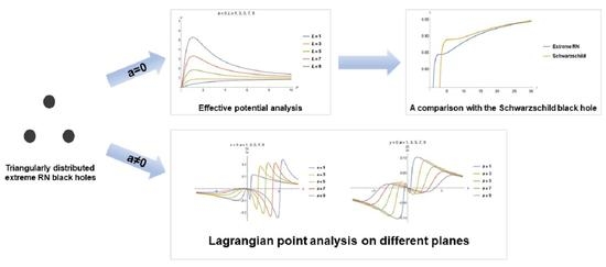
4. Effective Potential Analysis

Since the triangularly distributed black holes do not have spatial rotational symmetry, we cannot determine the angular momentum. In order to analyze the effective potential of TBH spacetime, we discuss the cases of a = 0 and $a\ne 0$, respectively.

4.1. $a=0$

When the separation distance a = 0, the three black holes merge into an extreme RN black hole. In this particular case, the spacetime model has rotational symmetry, so we use cylindrical coordinates, and the metric is transformed into:

$${ds}^2=-\frac{{dt}^2}{U^2}+U^2({d\rho }^2{+{\rho }^{2}d\phi }^2+{dz}^2),$$

(26)

where

$$U=1+\frac{M1+M2+M3}{\sqrt{{\rho }^2+z^2}}.$$

(27)

For the convenience of calculation, we set $M1=M2=M3=\frac{1}{3}$.

At this time the Lagrangian is:

$$\mathcal{L}=\frac{1}{2}{g}_{\mu \nu }{\dot{x}}^{\mu }{\dot{x}}^{\nu }=\frac{1}{2}[-\frac{\dot{t}}{U^2}+U^2({\dot{\rho }}^2+{\rho }^2{\dot{\phi }}^2+{\dot{z}}^2)].$$

(28)

Since spacetime is static and axisymmetric at this time, the Lagrangian is independent of the coordinates t and $\phi$, so we get two conserved quantities:

$$E=-\frac{\dot{t}}{U^2}L={\rho }^2{U}^2\dot{\phi }.$$

(29)

In Section 1, we give the four-speed normalization condition:

$$g_{\mu \nu }{\dot{x}}^{\mu }{\dot{x}}^{\nu }=\kappa .$$

(30)

According to these two conserved quantities and the normalization condition, we obtain the effective potential on the $\rho -z$ plane:

$${\dot{\rho }}^2+{\dot{z}}^2+V=E^2$$

(31)

$$V(\rho ,z;L^2)=\frac{L^2}{{\rho }^2{U}^4}+\frac{\kappa }{U^2}.$$

(32)

For time-like particles, we obtain the one-dimensional effective potential Figure 7 of the test particles on the $\rho -z$ plane:

It can be seen that with the increase of angular momentum that the image of the effective potential gradually moves up, and the inflection point of the function image will become more and more obvious.

Then, we get a two-dimensional effective potential Figure 8:

In order to obtain the innermost stable circular orbit in this case, we set:

$$\frac{dV}{d\rho }=0;\frac{d^{2}V}{d{\rho }^2}=0.$$

(33)

Finally, we calculate that when the separation distance is 0, the innermost stable circular orbit and the corresponding angular momentum are:

$$r_{ISCO}=3,L=2.82843.$$

(34)

Next, we compare the effective potential in this case and ISCO with the Schwarzschild black hole. For the convenience of calculation, we give the effective potential expression of the dimensionless quantity of the Schwarzschild black hole:

$$V_s=1-\frac{2}{r}+\frac{L^2}{r^2}-\frac{2L^2}{r^3}$$

(35)

by computing:

$$\frac{d{V}_s}{dr}=0;\frac{d^2{V}_s}{d{r}^2}=0.$$

(36)

We can get the innermost stable orbit radius of the Schwarzschild black hole and the corresponding angular momentum:

$$r_{sISCO}=6,L_s=2\sqrt{3}.$$

(37)

Figure 9 and Figure 10 show the one-dimensional and two-dimensional effective potential images of the extreme RN black hole and the Schwarzschild black hole at $L=2.82843$ and $L_s=2\sqrt{3}$.

4.2. $a\ne 0$

Next, we discuss the case $a\ne 0$. Because of $a\ne 0$, the extreme RN black hole system with triangular symmetric distribution has no spatial rotational symmetry. At this time, L is no longer a conserved quantity, and the exploration of the innermost stable circular orbit of TBH is meaningless. The innermost stable circular orbit will no longer exist. However, the Lagrangian point of this system does exist, so we will discuss the Lagrangian point in TBH spacetime.

Exploration of Lagrangian Point

We take time-like particles as an example. We already know the expression of the effective potential energy:

$$V(x,y,L^2)=\frac{L^2}{\left(x^2+y^2\right)U^4}+\frac{\kappa }{U^2}.$$

(38)

Since there is no symmetry of the three black holes on the $z=0$ plane, we explore the Lagrangian points on the x plane and the y plane, respectively. Since there is no angular velocity at the stable point, we do not need to consider the angular momentum, that is:

$$L=0.$$

(39)

First, we can get some fixed values by analyzing the x plane:

$$x=0,\kappa =1,a=5.$$

(40)

We can solve the following partial differential equations to obtain the Lagrangian point:

$$\frac{\partial V}{\partial y}=0.$$

(41)

Two solutions can be obtained:

$$y_1=-0.82,y_2=0.$$

(42)

In order to obtain more specific values, we need to change the different separation distance. Figure 11 shows the relationship between the Lagrange point and the separation distance a on the x plane. After verification, we can know that this figure can show the correct Lagrange point.

On the $y=0$ plane, we use the same method:

$$\frac{\partial V}{\partial x}=0.$$

(43)

The results are shown in Figure 12. Next, we take $a=5$ into the partial differential equation and we can see that the result is consistent with the figure:

$$x_1=2.23,x_2=-2.23,x_3=0.$$

(44)

According to the expression of the effective potential, we can see that, when $L=0$, the coordinate corresponding to the local minimum point is the zero point of the above equation.

5. Summary and Discussion

We studied the space-time properties under TBH, including the derivation of the space-time metric, the calculation of curvature scalar and curvature tensor, and the relationship between coordinate quantity and intrinsic quantity. Then, we found that, although coordinate quantity has no practical significance, it is of great significance for verifying the correctness of general relativity. Then, we analyzed the effective potential and the innermost stable circular orbit in the case of a = 0 and $a\ne 0$. When a = 0, we find that this is a special case. At this time, the TBH system can be regarded as an extreme RN black hole. We compared it with the effective potential and the innermost stable circular orbit radius of the standard Schwarzschild black hole. We found that the effective potential of TBH has a very important relationship with the separation distance and angular momentum. In a certain range, the larger the angular momentum, the higher the minimum value of the effective potential. When $a\ne 0$, we find that, since the system is no longer rotationally symmetric, there is no innermost stable circular orbit, but there is a Lagrangian point. We also analyzed the graph of the two-dimensional effective potential and found that the inflection point of the two-dimensional effective potential is closely related to the Lagrangian point, and the point corresponding to the Lagrangian point is the extreme point of the effective potential. The exploration of the Lagrangian point helps us to analyze the spatiotemporal properties of TBH more conveniently.

References

1. Misner, C.W.; Thorne, K.S.; Wheeler, J.A. Gravitation; W. H. Freeman and Co.: San Francisco, CA, USA, 1973. [Google Scholar]
2. Brenneman, L. Measuring the Angular Momentum of Supermassive Black Holes; Springer Briefs in Astronomy; Springer: New York, NY, USA, 2013. [Google Scholar]
3. Abramowicz, M.A.; Fragile, P.C. Foundations of Black Hole Accretion Disk Theory. Living Rev. Relativ. 2013, 16, 1. [Google Scholar] [CrossRef]
4. Abramowicz, M.A.; Jaroszyński, M.; Kato, S.; Lasota, J.-P.; Różańska, A.; Sądowski, A. Leaving the innermost stable circular orbit: The inner edge of a black-hole accretion disk at various luminosities. Astron. Astrophys. 2010, 521, A15. [Google Scholar] [CrossRef]
5. Galtsov, D.V.; Petukhov, V.I. Black hole in an external magnetic field. Sov. Phys. JETP 1978, 47, 419. [Google Scholar]
6. Aliev, A.N.; Gal’tsov, D.V. “Magnetized” black holes. Sov. Phys. Usp. 1989, 32, 75. [Google Scholar] [CrossRef]
7. Aliev, A.N.; Özdemir, N. N2002MNRAS. Motion of charged particles around a rotating black hole in a magnetic field. Mon. Not. R. Astron. Soc. 2002, 336, 241. [Google Scholar] [CrossRef]
8. Zahrani, A.M.A. Escape of charged particles moving around a weakly magnetized Kerr black hole. Phys. Rev. D 2014, 90, 044012. [Google Scholar] [CrossRef]
9. Pugliese, D.; Quevedo, H.; Ruffini, R. General classification of charged test particle circular orbits in Reissner–Nordström spacetime. Eur. Phys. J. C 2017, 77, 206. [Google Scholar] [CrossRef]
10. Pugliese, D.; Quevedo, H.; Ruffini, R. Motion of charged test particles in Reissner-Nordström spacetime. Phys. Rev. D 2011, 83, 104052. [Google Scholar] [CrossRef]
11. Wald, R.M. General Relativity; University of Chicago Press: Chicago, IL, USA, 1984. [Google Scholar]
12. Chandrasekhar, S. The Mathematical Theory of Black Holes; Oxford University Press: Oxford, UK, 1983. [Google Scholar]
13. Hartle, J.B.; Hawking, S.W. Solutions of the Einstein-Maxwell equations with many black holes. Commun. Math. Phys. 1972, 26, 87–101. [Google Scholar] [CrossRef]
14. Chandrasekhar, S. The two-centre problem in general relativity: The scattering of radiation by two extreme Reissner–Nordström black-holes. Proc. R. Soc. A 1989, 421, 227. [Google Scholar]
15. Abbott, B.P.; Abbott, R.; Abbott, T.D.; Abernathy, M.R.; Acernese, F.; Ackley, K.; Adams, C.; Adams, T.; Addesso, P.; Adhikari, R.X.; et al. (LIGO Scientific and Virgo Collaborations). Observation of Gravitational Waves from a Binary Black Hole Merger. Phys. Rev. Lett. 2016, 116, 061102. [Google Scholar] [CrossRef] [PubMed]
16. Abbott, B.P.; Abbott, R.; Abbott, T.D.; Abernathy, M.R.; Acernese, F.; Ackley, K.; Adams, C.; Adams, T.; Addesso, P.; Adhikari, R.X.; et al. (LIGO Scientific and Virgo Collaborations). Properties of the Binary Black Hole Merger G- W150914. Phys. Rev. Lett. 2016, 116, 241102. [Google Scholar] [CrossRef] [PubMed] [Green Version]
17. Abbott, B.P.; Abbott, R.; Adhikari, R.X.; Ananyeva, A.; Anderson, S.B.; Appert, S.; Arai, K.; Araya, M.C.; Barayoga, J.C.; Barish, B.C.; et al. Multi-messenger Observations of a Binary Neutron Star Merger. Astrophys. J. 2017, 848, L12. [Google Scholar] [CrossRef]
18. Abbott, B.P.; Abbott, R.; Abbott, T.D.; Abraham, S.; Acernese, F.; Ackley, K.; Adams, C.; Adhikari, R.X.; Adya, V.B.; Affeldt, C.; et al. (LIGO Scientific and Virgo Collaborations). GWTC-1: A Gravitational-Wave Transient Catalog of Compact Binary Mergers Observed by LIGO and Virgo During the First and Second Observing Runs. Phys. Rev. X 2019, 9, 031040. [Google Scholar]
19. Weyl, H. The theory of gravitation. Ann. Phys. 1917, 359, 117. [Google Scholar] [CrossRef]
20. Majumdar, S.D. A Class of Exact Solutions of Einstein’s Field Equations. Phys. Rev. 1947, 72, 390–398. [Google Scholar] [CrossRef]
21. Papaetrou, A. A static solution of the equations of the gravitational field for an arbitrary charge distribution. Proc. R. Irish Acad. Sect. A 1947, 51, 191. [Google Scholar]
22. Kramer, D.; Neugebauer, G. The superposition of two Kerr solutions. Phys. Lett. A 1980, 75, 259–261. [Google Scholar] [CrossRef]
23. Nitta, D.; Chiba, T.; Sugiyama, N. Shadows of colliding black holes. Phys. Rev. D 2011, 84, 063008. [Google Scholar] [CrossRef]
24. Bohn, A.; Throwe, W.; Hébert, F.; Henriksson, K.; Bunandar, D.; A Scheel, M.; Taylor, N.W. What does a binary black hole merger look like? Class. Quantum Gravity 2015, 32, 065002. [Google Scholar] [CrossRef]
25. Patil, M.; Mishra, P.; Narasimha, D. Curious case of gravitational lensing by binary black holes: A tale of two photon spheres, new relativistic images, and caustics. Phys. Rev. D 2017, 95, 024026. [Google Scholar] [CrossRef]
26. Assumpção, T.; Cardoso, V.; Ishibashi, A.; Richartz, M.; Zilhão, M. Black hole binaries: Ergoregions, photon surfaces, wave scattering, and quasinormal modes. Phys. Rev. D 2018, 98, 064036. [Google Scholar] [CrossRef]
27. Cunha, P.V.P.; Herdeiro, C.A.R.; Rodriguez, M.J. Shadows of exact binary black holes. Phys. Rev. D 2018, 98, 044053. [Google Scholar] [CrossRef]
28. Campanelli, M.; Dettwyler, M.; Hannam, M.; Lousto, C.O. Relativistic three-body effects in black hole coalescence. Phys. Rev. D 2006, 74, 087503. [Google Scholar] [CrossRef] [Green Version]
29. Torigoe, Y.; Hattori, K.; Asada, H. Gravitational Wave Forms for Two- and Three-Body Gravitating Systems. Phys. Rev. Lett. 2009, 102, 251101. [Google Scholar] [CrossRef] [PubMed]
30. Seto, N. Relativistic resonant relations between massive black hole binary and extreme mass ratio inspiral. Phys. Rev. D 2012, 85, 064037. [Google Scholar] [CrossRef]
31. Yamada, K.; Asada, H. Nonchaotic evolution of triangular configuration due to gravitational radiation reaction in the three-body problem. Phys. Rev. D 2016, 93, 084027. [Google Scholar] [CrossRef]
32. Hayasaki, K.; Mineshige, S.; Sudou, H. Binary Black Hole Accretion Flows in Merged Galactic Nuclei. Publ. Astron. Soc. Jpn. 2007, 59, 427–441. [Google Scholar] [CrossRef]
33. Hayasaki, K.; Mineshige, S.; Ho, L.C. A Supermassive Binary Black Hole with Triple Disks. Astrophys. J. 2008, 682, 1134–1140. [Google Scholar] [CrossRef]
34. Novikov, I.D.; Thorne, K.S. Astrophysics of Black Holes, in Black Holes (Les Astres Occus); DeWitte, C., DeWitt, B., Eds.; Gordon and Breach: New York, NY, USA, 1973; p. 343. [Google Scholar]
35. Clark, J.P.A.; Eardley, D.M. Evolution of close neutron star binaries. Astrophys. J. 1977, 215, 311–322. [Google Scholar] [CrossRef]
36. Kidder, L.E.; Will, C.M.; Wiseman, A.G. Coalesc- ing binary systems of compact objects to epostT 5=2 Newtonian order. III. Transition from inspiral to plunge. Phys. Rev. D 1993, 47, 3281. [Google Scholar] [CrossRef] [PubMed]
37. Nakashi, K.; Igata, T. Effect of a second compact object on stable circular orbits. Phys. Rev. D 2019, 100, 104006. [Google Scholar] [CrossRef] [Green Version]
Figure 1. This is the Lagrangian point distribution of the Earth-Moon system, m1 is the Earth and m2 is the Moon.
Symmetry 15 00505 g001
Figure 2. The three black holes are distributed as shown in this diagram, and they are all distributed at a distance from each other in an equilateral triangle.
Symmetry 15 00505 g002
Figure 3. This is a two-dimensional graph of curvature scalars on the x, y, and z planes respectively, where (a) is the x = 0 plane, (b) is the y= 0 plane, and (c) is the z= 0 plane.
Symmetry 15 00505 g003
Figure 4. This is a three-dimensional diagram of the relationship between the coordinate distance and the inherent distance. Figure (a) shows their local relationship and then figure (b) shows the global relationship.
Symmetry 15 00505 g004
Figure 5. This is a three-dimensional graph of the relationship between the coordinate time and the intrinsic time. Figure (a) shows the local and figure (b) shows the global relationship.
Symmetry 15 00505 g005
Figure 6. This is the distribution of the radial coordinate velocity in the Cartesian coordinate system. At infinity, the coordinate velocity is equal to the intrinsic velocity.
Symmetry 15 00505 g006
Figure 7. This is a one-dimensional effective potential image of the test particle on the ρ z plane. Since this is a special case (a = 0), we observe it by changing the angular momentum. The blue line represents L = 1 , the orange line represents L = 3 , the green line represents L = 5 , the red line represents L = 7 , and the purple line represents L = 9 .
Symmetry 15 00505 g007
Figure 8. We selected the two-dimensional effective potential of particles in the z plane under different angular momentum. The orange image represents L = 2.82348 , the blue area represents L = 5 , and the green area represents L = 10 . It can be seen that, as the effective potential increases, the image position of the two-dimensional effective potential will also rise.
Symmetry 15 00505 g008
Figure 9. This is the one-dimensional effective potential image of extreme RN black hole and Schwarzschild black hole in L = 2.82843 .
Symmetry 15 00505 g009
Figure 10. This is a figure of the two-dimensional effective potential of the Schwarzschild black hole and the extreme RN black hole from different perspectives. Figure (a) is a top view and figure (b) is a positive attempt. The orange region is the Schwarzschild black hole, and the blue region is the extreme RN black hole. We can clearly see that the radius of the innermost stable circular orbit of the Schwarzschild black hole is larger than that of the extreme RN black hole.
Symmetry 15 00505 g010
Figure 11. This is the relationship between the Lagrangian point and the separation distance a on the x axis. When the separation distance changes, the Lagrangian point also changes.
Symmetry 15 00505 g011
Figure 12. This is the relationship between the Lagrangian point and the separation distance a on the y axis. When a = 5 , the corresponding Lagrangian point coordinates are as we calculated.
Symmetry 15 00505 g012
Disclaimer/Publisher’s Note: The statements, opinions and data contained in all publications are solely those of the individual author(s) and contributor(s) and not of MDPI and/or the editor(s). MDPI and/or the editor(s) disclaim responsibility for any injury to people or property resulting from any ideas, methods, instructions or products referred to in the content.